Isobaric first-principles molecular dynamics of liquid water with nonlocal van der Waals interactions

Abstract

We investigate the structural properties of liquid water at near ambient conditions using first-principles molecular dynamics simulations based on a semilocal density functional augmented with nonlocal van der Waals interactions. The adopted scheme offers the advantage of simulating liquid water at essentially the same computational cost of standard semilocal functionals. Applied to the water dimer and to ice I${}_{\textrm{h}}$, we find that the hydrogen-bond energy is only slightly enhanced compared to a standard semilocal functional. We simulate liquid water through molecular dynamics in the $NpH$ statistical ensemble allowing for fluctuations of the system density. The structure of the liquid departs from that found with a semilocal functional leading to more compact structural arrangements. This indicates that the directionality of the hydrogen-bond interaction has a diminished role as compared to the overall attractions, as expected when dispersion interactions are accounted for. This is substantiated through a detailed analysis comprising the study of the partial radial distribution functions, various local order indices, the hydrogen-bond network, and the selfdiffusion coefficient. The explicit treatment of the van der Waals interactions leads to an overall improved description of liquid water.

I Introduction

Understanding the structural and dynamical properties of liquid water is of great importance due to its ubiquity in biological and chemical processes. Nevertheless, giving a comprehensive picture of water and aqueous solutions at the molecular level still represents a noticeable challenge. Molecular dynamics simulations based on empirical force fields have long been the technique of choice for investigating the microscopical properties of aqueous solutions.Jorgensen et al. (1983); Mahoney and Jorgensen (2000) However, force field methods rely on experimental data and the results depend on how the force field is parametrized. Furthermore, the parametrization varies from one system to another leading to a transferability problem. These limitations are overcome by simulation schemes based on first-principles density functionals, in which the energy and the atomic forces are evaluated directly from the evolving electronic structure.

With the increasing availability of computer resources and the improvement of computational algorithms, first-principles techniques have been extensively applied to study the structural and dynamical properties of liquid water.Laasonen et al. (1993); Sprik, Hutter, and Parrinello (1996); Izvekov and Voth (2002); Grossman et al. (2003); VandeVondele et al. (2004); Sit and Marzari (2005); Lee and Tuckerman (2007); Schmidt et al. (2009) It has become clear that density functionals in which the exchange-correlation energy is treated within a generalized gradient approximation lead to overstructured systems and to underestimated diffusion coefficients. When the description of the electronic structure is improved through the use of hybrid density functionals, these shortcomings persist.Todorova et al. (2006); Guidon et al. (2008) Similarly, the explicit consideration of the quantum motion of the nuclei is not sufficient to lead to a significant amelioration of the structural properties.Morrone and Car (2008) At variance, recent studies have pointed to the critical importance of accounting for van der Waals interactions in the description of liquid water.Grimme (2004); Dion et al. (2004); *dion_ePRL2005; Thonhauser et al. (2007); Lee et al. (2010); Cooper (2010); Vydrov and Van Voorhis (2010)

Sophisticated methods such as coupled clusters or Møller-Plesset perturbation theory accurately account for van der Waals interactions and have recently been applied to liquid water.Del Ben et al. (2013) However, these methods are still computationally too demanding for a widespread use in routine simulations. More recently, several strategies for including van der Waals interactions within density functional simulation schemes have been proposed leading to an improved description of the structural and dynamical properties of liquid water.Lin et al. (2009); Schmidt et al. (2009); Wang et al. (2011); Lin et al. (2012) In particular, Schmidt et al. performed molecular dynamics simulations of liquid water in the isobaric-isothermal ensemble ($NpT$).Schmidt et al. (2009) In $NpT$ simulations, the supercell parameters are free to adjust during the evolution allowing the system to reach its equilibrium density at a fixed pressure without imposing additional constraints. These simulationsSchmidt et al. (2009) revealed that the equilibrium density yielded by semilocal density functionals underestimates the experimental value by about 15% and that the experimental density is recovered through the use of empirical dispersion corrections.Grimme (2004) These results are in perfect agreement with the molecular dynamics simulations performed by Wang et al.,Wang et al. (2011) who compared semilocal and van der Waals corrected density functionals using a $NVT$ protocol.

Recently, several nonlocal formulations have been introduced which explicitly account for van der Waals interactions through a functional of the density.Dion et al. (2004); Tkatchenko and Scheffler (2009); Lee et al. (2010); Vydrov and Van Voorhis (2010) Among these, the one proposed by Vydrov and Van VoorhisVydrov and Van Voorhis (2010) in its revised form denoted rVV10 carries the advantage of being particularly suited to be used in conjunction with plane-wave basis sets, leading to a scheme which does not yield any significant overhead with respect to standard semilocal functionals.Sabatini, Gorni, and de Gironcoli (2013) While rVV10 still relies on a phenomenological formulation, it carries an important advantage with respect to empirical schemes. Indeed, once the parameters are set, the resulting functional can be carried over to any weakly bonded system without requiring any further parameter tuning. It could thus be envisaged to use the same theoretical scheme for studying various aqueous solutions.

In this work, we present results obtained through first-principles molecular dynamics simulations in the $NpH$ ensemble of liquid water at near ambient conditions. The van der Waals interactions are explicitly taken into account through the functional rVV10.Vydrov and Van Voorhis (2010); Sabatini, Gorni, and de Gironcoli (2013) First, we test the performance of the rVV10 functional on the water dimer and on the I${}_{\textrm{h}}$ phase of ice, finding only small variations of the hydrogen bond strength in those systems compared to semilocal functionals. In our molecular dynamics simulations of liquid water, we then find that rVV10 provides a noticeably improved description compared to standard semilocal functionals. Not only the equilibrium density is recovered but also the structural and dynamical properties are much closer to experimental observations. In particular, we focus on the local order and on an analysis of the hydrogen bond network. Hence, rVV10 allows for a good description of liquid water at a computational cost equivalent to semilocal density functionals and appears particularly attractive for the treatment of water-solute interactions.

The present paper is organized as follows. In Sec. II, we describe the methods used in this work and give a detailed account of our simulation protocols. In Secs. III and IV, we apply rVV10 to the water dimer and the I${}_{\textrm{h}}$ phase of ice, respectively. The results for liquid water and the corresponding analyses are given in Sec. V. The conclusions are drawn in Sec. VI.

II Methods

II.1 Computational details

The computational scheme adopted throughout this work is based on the self-consistent Kohn-Sham approach to density functional theory (DFT) as implemented in the Quantum-espresso suite of programs.Giannozzi et al. (2009) The valence Kohn-Sham orbitals are expanded up to a kinetic-energy cutoff of 85 Ry, while core-valence interactions are described by norm-conserving pseudopotentials.Troullier and Martins (1991) The exchange-correlation (XC) energy is described within the generalized-gradient approximation proposed by Perdew, Becke, and Ernzerhof (PBE).Perdew, Burke, and Ernzerhof (1996) In addition to the semilocal PBE functional, we performed calculations in which van der Waals interactions are explicitly taken into account. To this aim, among the several van der Waals density functional schemes proposed, we adopted rVV10 functional, recently introduced by Sabatini et al.Sabatini, Gorni, and de Gironcoli (2013) as an essentially equivalent variant of the nonlocal VV10 functional developed by Vydrov and Van Voorhis.Vydrov and Van Voorhis (2010) The VV10 functional has been shown to be particularly successful in reproducing the physical properties of molecules and weakly bonded solids.Vydrov and Van Voorhis (2010); Hujo and Grimme (2011) The advantage of adopting the revised functional rVV10 rests in a more efficient evaluation of the correlation energy and its derivatives within a plane-waves framework, a major prerequisite when long ab initio molecular dynamics simulations have to be carried out.

The rVV10 functional is defined by a very simple analytic form and depends on an empirically determined parameter, $b$, which controls the short-range behavior of the functional.Vydrov and Van Voorhis (2010); Sabatini, Gorni, and de Gironcoli (2013) This parameter can be optimized in order to reproduce the correct physical properties of a chosen set of materials. In particular, the rVV10 functional, as implemented in the Quantum-espresso package, has been tested over the S22 set of molecules. The best description of the binding energies is obtained for $b=6.3$.Sabatini, Gorni, and de Gironcoli (2013) Although accurate in describing the binding energy and geometry of molecules,Vydrov and Van Voorhis (2010); Hujo and Grimme (2011) the VV10 functional gives overestimated binding energies for weakly bonded solids.Björkman et al. (2012) To achieve an improved description of a set of layered solids, Björkman has proposed a higher value for the parameter $b$ (up to 10.25).Björkman (2012) To identify the optimal functional for treating aqueous systems, we therefore consider in the following various values of the parameter $b$.

II.2 Molecular dynamics simulations

We perform first-principles Born-Oppenheimer molecular dynamics simulations of 64 water molecules in the isobaric-isoenthalpic statistical ensemble ($NpH$) at near-ambient conditions. The quantum motion of the nuclei is neglected in the present work. We use the Beeman algorithm to integrate Newton’s equations of motion, as implemented in the Quantum-espresso package, with an integration time step of 0.48 fs. Simulations are carried out using the PBE and rVV10 functionals. In the latter, the parameter $b$ is set to 6.3, 8.9, 9.3, and 9.5, respectively. In the following, we use the notation rVV10-b6.3 to indicate the rVV10 functional with the parameter $b$ set to 6.3, and similarly for the other values of $b$. The molecular dynamics runs last between 25 and 35 ps. The cell size is allowed to fluctuate with the constraint of conserving the initial cubic symmetry. A vanishing external pressure is imposed through the use of the Parrinello-Rahman barostat.Parrinello and Rahman (1980)

The starting configuration for each simulation is chosen from a trajectory obtained through a $NVT$ classical molecular-dynamics simulation in which the density of the system is fixed at 1 g/cm³ and the temperature at 300 K. For each functional, a preliminary $NpT$ equilibration run of about 5 ps is carried out before collecting statistics. The temperature is set to 350 K to ensure a liquid-like behavior VandeVondele et al. (2004); Sit and Marzari (2005); Schwegler, Galli, and Gygi (2000) During the equilibration runs the temperature is controlled by a velocity rescaling thermostat, which only acts when the cumulative average temperature moves out of the window 350$\pm$20 K. However, we observe that the temperature drift during the equilibration time is minimal and that the thermostat remains inactive after an initial period of a few picoseconds. In particular, we obtained average temperatures of 349, 344, and 342 K for our molecular dynamics simulations based on PBE, rVV10-b6.3, rVV10-b9.3, respectively.

In the $NpT$ molecular dynamics simulations with a basis set involving a constant number of plane waves, fluctuations of the volume imply fluctuations of the effective energy cutoff defining the basis set.Bernasconi et al. (1995) This condition requires extra precautions. All the simulations are started from a geometry with a cell of fixed density at 1 g/cm³ and the corresponding cut-off energy is chosen in such a way that the stress tensor is converged within 1 kbar. Those simulations, which show a decrease of density during the equilibration run, are restarted with a larger initial volume to restore the originally set higher cut-off. Once the cumulative average value of the density reaches a constant value, we ensure that the density fluctuations do not lead to any integration problem.

During all the production runs, we observe that the temperature remains constant and that the conditions to activate the thermostat are not met. In these conditions our simulations are effectively sampling the isobaric-isoenthalpic ($NpH$) ensemble. Since the external pressure is forced to be zero the total energy of the system, $E$, is conserved on average and can be used to check the quality of our integration scheme.

III Water dimer

The simplest system that water molecules can form is the water dimer. Despite its simplicity, the water dimer has extensively been investigated in physical chemistry.Dyke, Mack, and Muenter (1977); Odutola and Dyke (1980) It plays a major role in many important physical and chemical processes. In addition, a better understanding of the isolated water dimer implies a better understanding of the hydrogen bond which is at the origin of the very peculiar properties of water in its condensed phases.Jeffrey (1997) Finally, in simulation studies, the water dimer is often used as the simplest water system to test new computational approaches.Kim and Jordan (1994); Feyereisen, Feller, and Dixon (1996)

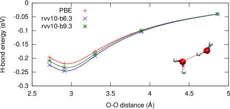
Figure 1: Binding energy of the water dimer as a function of the intermolecular separation calculated with the PBE, rVV10-b6.3, and rVV10-b9.3 functionals. The water dimer geometry is shown in the inset.

In Fig. 1, we report the binding energy of the water dimer as a function of the inter-molecular separation, as calculated with various functionals. The binding energies are obtained for a dimer with fixed geometries in a cubic supercell with lattice parameter of 20 Å. We took as our reference structure the optimized geometry obtained in Ref. 41 through the coupled cluster CCSD(T) method in the complete basis set limit. The structures with other O-O distances, were then obtained by displacing one of the H₂O molecules while preserving the symmetry and keeping the the angle along the H-bond, $\angle$O$\cdots$HO, fixed and equal to its value in the reference configuration, $\alpha=172.8^{\circ}$. The other structural parameters were not varied with respect to the reference structure. The reference dimer geometry is shown in the inset of Fig. 1.

Table 1: Binding energy of the water dimer calculated with the PBE, rVV10-b6.3, and rVV10-b9.3 functionals.

	$E_{0}$/H2O (eV)
PBE	0.22
rVV10-b6.3	0.25
rVV10-b9.3	0.23
CCSD(T)Jurečka et al. (2006)	0.22

The optimized CCSD(T) configuration gives the minimum binding energy for all our DFT calculations at the same geometry. The obtained values are given in Table 1. Among the DFT calculations, PBE gives the best agreement with our reference calculation.Jurečka et al. (2006) However, the binding energies obtained with the various VV10 variants increase by at most 0.03 eV. For each of the DFT functionals, we check that a full structural relaxation leads to energy differences of less than 5 meV without causing any significant structural modification with respect to the reference configuration. These results indicate that all the considered DFT functionals account well for the strength of the H-bond and for the geometry of the water dimer.

IV I${}_{\textrm{h}}$ phase of ice

We next investigate the effect of including van der Waals interactions on the H-bond strength, cohesive energy, and structural properties of ice. The performance of the semilocal PBE and the various rVV10 functionals are compared among each other and against experimental and theoretical data.

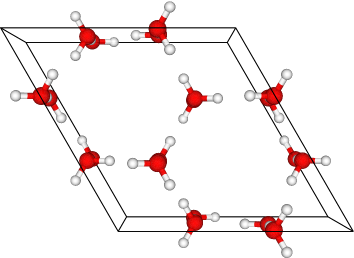
Figure 2: Perspective view along the $c$ axis of the Bernal-Fowler model of ice I${}_{\textrm{h}}$.

At present, several ice phases have been experimentally characterized. The oxygen atoms are always found in an ordered sublattice and the water molecules are orientated in such a way that the O atoms are approximately tetrahedrally coordinated by four H atoms, two of which are bonded covalently while the other two belong to nearest-neighbor water molecules and are bonded through hydrogen bonds. This “ice rule” is always satisfied even if the varying orientation of the water molecules may lead to disordered networks lacking any form of translational invariance. The various ice structures therefore mainly differ by the form of the hydrogen-bond network and the packing density.

For our purpose, we use the periodic model of the I${}_{\textrm{h}}$ phase proposed by Bernal and Fowler.Bernal and Fowler (1933) This model of ice has been adopted in several theoretical studies to test the accuracy of density functionals in describing solid water networks.Hamann (1997); Kolb and Thonhauser (2011); Santra et al. (2013) Figure 2 shows a top-view perspective along the $c$ axis of the ordered Bernal-Fowler model of ice. The unit cell contains 12 water molecules and belongs to the P6₃cm(C${}^{3}_{6v}$) space group. Following Hamann,Hamann (1997) we adopt the experimental cell ratio $c/a$, which ensures that all hydrogen bonds have the same length. The Brillouin-zone is sampled using a 2$\times$2$\times$2 Monkhorst-Pack grid which does not include the $\Gamma$-point.

In Fig. 3, the calculated sublimation energies as a function of the volume per water molecule are plotted for PBE, rVV10-b6.3, and rVV10-b9.3 functionals. In this calculation, the $c/a$ is not allowed to change. The energetics and the equilibrium structural properties of ice I${}_{\textrm{h}}$ are reported in Table 2. The PBE functional gives a sublimation energy of 0.63 eV, slightly larger than the experimental value of 0.61 eV. This result is in good agreement with previous theoretical results which generally overestimate the experimental value by an amount ranging between 30 and 100 meV per H₂O molecule. In particular, it is noteworthy that our results agree closely with the highly converged projector-augmented-wave calculations reported in Ref. 46. The account of van der Waals interactions leads to an even larger overestimation of the experimental results. This result qualitatively agrees with a previous theoretical investigation of ice I${}_{\textrm{h}}$ by Santra et al.Santra et al. (2013) However, as can be seen in Table 2, a general improvement is achieved when the phenomenological parameter $b$ in the rVV10 formulation is set to 9.3 rather than to its original value of 6.3.

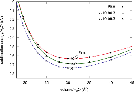
Figure 3: Sublimation energies per H₂O molecule vs. volume for ice I${}_{\textrm{h}}$ as obtained with PBE, rVV10-b6.3, rVV10-b9.3 functionals. The minima of the Murnaghan equation of state are marked and the experimental value is reported for comparison.Whalley (1984); Brill and Tippe (1967)

Table 2: Sublimation energy per H₂O molecule $E_{0}$, equilibrium volume per H₂O molecule $V_{0}$, and bulk modulus $B$ of ice I${}_{\textrm{h}}$ as obtained with PBE, rVV10-b6.3, and rVV10-b9.3 functionals.

	$E_{0}$ (eV)	$V_{0}$ (Å3)	$B$ (GPa)
PBE	0.63	31.03	13.2
rVV10-b6.3	0.74	30.86	16.2
rVV10-b9.3	0.69	31.44	15.6
Expt.Whalley (1984); Brill and Tippe (1967); Hobbs	0.61	32.05	10.9

V Liquid water

We here present our results obtained through molecular dynamics simulations of liquid water near-ambient conditions using both semilocal and van der Waals corrected density functionals. All the data presented here are the result of statistical analyses performed on molecular dynamics trajectories having duration between 25 and 35 ps. For technical details of the simulations we refer the reader to Sec. II.2.

V.1 Equilibrium density

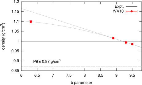
Figure 4: Equilibrium density of liquid water at near-ambient condition as obtained from rVV10 simulations with different values of the empirical $b$ parameter. For comparison, the equilibrium densities obtained in the experiment and in simulations based on the PBE functional are also reported. All the simulations show average temperatures falling within the range $345\pm 4$ K. The solid horizontal line indicates the density of liquid water at 4^∘C (1 g/cm³).

Isobaric molecular dynamics simulations allow for a direct evaluation of the equilibrium density of the system. We find that the PBE functional gives an average density for liquid water of $\sim$0.87 g/cm³ underestimating the experimental value by about 13%, in very good agreement with previous theoretical studies.Schmidt et al. (2009); Wang et al. (2011) In contrast, the explicit introduction of van der Waals interactions, described by the rVV10 functional with the parameter $b$ set to its original value of 6.3, causes an overestimation of the equilibrium density. We obtain a value of $\sim$1.10 g/cm³, about 10% higher than the experimental value. Figure 4 shows the average densities obtained with rVV10 simulations for various values of the parameter $b$. Our simulations give average densities of 1.10, 1.02, 0.99, and 0.98 g/cm³ for $b$=6.3, 8.9, 9.3, and 9.5, respectively. In particular, for the specific value of $b$=9.3 the simulation yields an average density which closely matches the experimental density of 1 g/cm³.

While a higher density clearly corresponds to more compact arrangements and to a partial breakdown of the hydrogen-bond network, this result does not come from a weakening of the hydrogen-bond strength. In Sec. III, we indeed show that the rVV10 functional leads to a slight increase of the hydrogen-bond energy when compared to the PBE one. Therefore, the more compact arrangements found with rVV10 necessarily come from alternative structural configurations which are more favored than in the PBE, due to the less directional nature of the attraction between the water molecules.

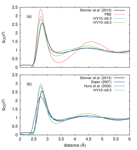
Figure 5: (a) The oxygen-oxygen radial distribution functions $g_{\textrm{OO}}(r)$ as obtained with PBE, rVV10-b6.3, and rVV10-b9.3 functionals are compared with the x-ray diffraction result of Skinner et al. from Ref. Skinner et al., 2013. (b) The $g_{\textrm{OO}}(r)$ as obtained with rVV10-b9.3 is compared with various experimental measurements.Skinner et al. (2013); Soper (2007); Hura et al. (2000) The average temperatures are 349, 344, 342 K for PBE, rVV10-b6.3, and b-9.3 simulations, respectively, while all the experimental results have been obtained at ambient temperature.

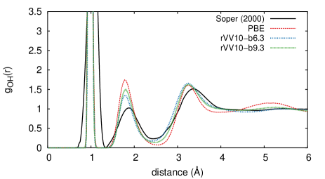
Figure 6: Oxygen-hydrogen radial distribution functions as obtained with PBE, rVV10-b6.3, and rVV10-b9.3 functionals are compared with the experimental result from Ref. 53. The average temperatures in the simulations are reported in the caption of Fig. 5.

V.2 Radial distribution functions

The oxygen-oxygen and oxygen-hydrogen radial distribution functions (RDF) as obtained with various functionals are compared with recent experimental resultsSkinner et al. (2013); Soper (2007); Hura et al. (2000); Soper (2000) in Figs. 5 and 6, respectively. For the radial distribution functions achieved with the PBE functional, one notices that the obtained description of liquid water is overstructured, in agreement with previous theoretical studies.Schmidt et al. (2009) Focusing on O-O correlations, Fig. 5(a), we remark that the position of the first peak at 2.75 Å in the simulated radial distribution function is in good agreement with the experimental position at 2.80 Å, but the second coordination shell is slightly shifted towards larger distances, and so is the second minimum.

An overall improved description is achieved for the rVV10 functionals. When the rVV10 functional is used in its original form with $b=6.3$, the agreement with the experimental result improves as far as the value of $g_{\textrm{OO}}^{\textrm{max}}$ is concerned. An improvement is also observed for the second solvation shell, where the $g_{\textrm{OO}}(r)$ is nevertheless less structured with respect to the experiment and the position of the peak is slightly shifted toward lower distances. The rVV10 functional with $b=9.3$ yields yet better positions of minima and maxima, but the $g_{\textrm{OO}}(r)$ is slightly overstructured. In Fig. 5(b), we compare the $g_{\textrm{OO}}(r)$ obtained with the rVV10-b9.3 functional with other experimental results in literature.Skinner et al. (2013); Soper (2007); Hura et al. (2000) This comparison shows the variation among the experimental results, but confirms that the $g_{\textrm{OO}}(r)$ obtained with the rVV10-b9.3 functional is slightly overstructured.

For oxygen-hydrogen correlations (Fig. 6), the rVV10 functionals similarly yield smoother radial distribution functions than the PBE, but the dependence on the parameter $b$ appears less pronounced. The closer agreement with experiment for the radial distribution functions is consistent with the improved description of the equilibrium density (cf. Sec. V.1).

The agreement with experiment achieved with the functional rVV10 is overall similar to that obtained with empirical van der Waals interactions.Schmidt et al. (2009) Simulations based on the rVV10 functional with values of the $b$ parameter ranging from 8.9 to 9.5 show structural properties with minimal differences. Therefore, we focus in the following only on results obtained with PBE, the original rVV10-b6.3, and rVV10-b9.3.

V.3 Local order

An analogy can be drawn between variations of the parameter $b$ in the rVV10 functional and variations of the external pressure. As shown in Fig. 4, the equilibrium density of liquid water ranges from 1.10 to 0.87 g/cm³ when going from a rVV10 simulation with the lowest value of the parameter $b$ to PBE. Accordingly, the liquid-water system undergoes an increase of the local order as can be inferred from the oxygen-oxygen radial distribution functions in Fig. 5. In order to give a microscopic interpretation of the density variations resulting from the tuning of the phenomenological parameter $b$, we perform statistical analyses of structural descriptors which give a measure of the local order.

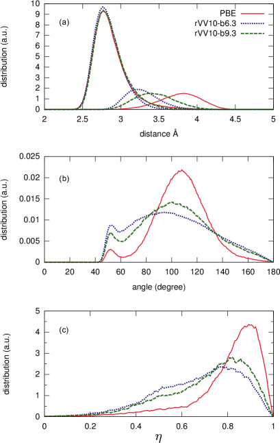
Figure 7: Distributions of local order parameters obtained with PBE, rVV10-b6.3, and rVV10-b9.3 functionals: (a) O-O distance within the first coordination shell, the first four neighbors and the fifth one are presented separately; (b) $\angle$ O-O${}_{\textrm{c}}$-O angle for an O-O${}_{\textrm{c}}$ cutoff distance of 3.5 Å; (c) orientational order parameter $\eta$ defined in Eq. 1.

We perform an analysis of the O-O distances between a water molecule and other water molecules belonging to its first solvation shell. For each instantaneous solvation shell around a central molecule, the neighboring molecules are ranked according to theses distances. The first four molecules are assumed to form the first coordination shell. As shown in Fig. 7(a), all the functionals considered in this work produce very similar distance distributions for the first coordination shell. At variance, the distribution of the fifth water molecule is highly sensitive to the adopted functional and moves closer to the central water molecule, as the contribution of the dispersion forces becomes more important. In the literature, this fifth water molecule is often interpreted as an “interstitial” molecule within the regular liquid water network.Saitta and Datchi (2003)

Additional insight into the local arrangement of water molecules can be acquired by inspecting the O-O${}_{\textrm{c}}$-O angle distributions given in Fig. 7(b), where the O${}_{\textrm{c}}$ atom belongs to the central molecule while the other O atoms belong to the solvation shell defined by an O-O${}_{\textrm{c}}$ cutoff distance of 3.5 Å. When compared to PBE, the rVV10 functionals favor a shift towards lower angles and a broadening of the main peak at about 109^∘. This clearly indicates a distortion of the tetrahedral geometry of the first coordination shell.

The tetrahedral distortion can be further investigated by the distribution of the orientational order parameter $\eta$ introduced in Ref. 55:

$$\eta=1-\frac{3}{8}\sum_{i=1}^{3}\sum_{j=i+1}^{4}\left(\cos\theta_{ij}+\frac{1}{3}\right)^{2}$$ (1)

where $\theta_{ij}$ is the angle between the vectors connecting the oxygen atom of the central molecule with two oxygen atoms belonging to its first four nearest-neighbors molecules. This parameter is defined in such a way that it assumes the value $\eta=1$ in a perfect tetrahedral geometry such as in ice I${}_{\textrm{h}}$, whereas $\eta=0$ in an ideal gas. As shown in Fig. 7(c), the PBE gives a distribution which peaks at a high value of $\eta$ around 0.9. When van der Waals interactions are explicitly accounted for, the main peak of the distribution shifts to lower values and a secondary feature appears around 0.5. In their original work, Errington and DebenedettiErrington and Debenedetti (2001) found that the relative weight of the second feature increased with temperature, i.e. with structural disorder. In our simulations, the enhanced weight of the second feature is related to the decrease of the parameter $b$, or in other words with the increase of the equilibrium density.

Another order parameter which is sensitive to the degree of local tetrahedral order is the local structure index (LSI) $I$ introduced in Refs. 56; 57. This parameter is expected to discriminate molecules with a well structured tetrahedral environment, with separated first and second shells, from molecules around which the order is perturbed by an approaching “interstitial” molecule.Shiratani and Sasai (1998); Palmer et al. (2014) For a given central molecule $\mu$, a neighboring oxygen atom $i$ is ranked and labelled according to the distance $r_{i}$ to the central molecule $\mu$, such that : $r_{1}<r_{2}<\dots<r_{i}<r_{i+1}<\dots<r_{n(\mu,t)}<r_{n(\mu,t)+1}$, where the number $n(\mu,t)$ satisfies the relation $r_{n(\mu,t)}<3.7\,\textrm{\AA}<r_{n(\mu,t)+1}$. The LSI $I(\mu,t)$ of the central molecule $\mu$ at time $t$ then reads:

$$I(\mu,t)=\frac{1}{n(\mu,t)}\sum_{i=1}^{n(\mu,t)}\left[\Delta(i;\mu,t)-\bar{\Delta}(\mu,t)\right]^{2},$$ (2)

where $\Delta(i;\mu,t)=r_{i+1}-r_{i}$ and $\bar{\Delta}(\mu,t)$ is the average obtained as

$$\bar{\Delta}(\mu,t)=\frac{1}{n(\mu,t)}\sum_{i=1}^{n(\mu,t)}\Delta(i;\mu,t).$$ (3)

The LSI describes the local inhomogeneity of a water molecule. A high local tetrahedral order corresponds to a high value of $I$. To characterize the local order, we thus calculate the index $\bar{I}$, averaged over all molecules and over time. For instance, one finds an average $\bar{I}=0.25$ Ų for the ice phase.Palmer et al. (2014) Instead, when the disorder prevails, the $\bar{I}\approx 0$.

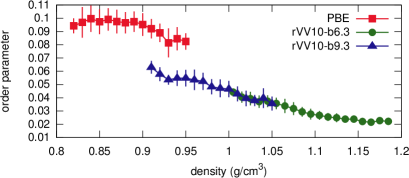
Figure 8: Average value of the local structure index (LSI) $I$ (Eq. 2) as a function of the instantaneous density, as obtained from PBE, rVV10-b6.3, and rVV10-b9.3 simulations. Vertical lines indicate the statistical error.

Figure 8 shows the behavior of the LSI as a function of the instantaneous density in our molecular dynamics simulations. Results obtained with different functionals are superposed. The PBE functional gives the lowest densities and the most ordered local structures with $\bar{I}=0.10$ Ų. The rVV10 simulations give $\bar{I}=0.03$ Ų and $\bar{I}=0.05$ Ų for $b=6.3$ and $b=9.3$, respectively. Interestingly, the two rVV10 simulations yield local structure indices which superpose continously as a function of density, suggesting that the $I$ vs. density behaviour is not sensitive to the parameter $b$ within the class of rVV10 functionals. Furthermore, it is worthwhile to point that the trend of LSI vs. density observed in this work is qualitatively consistent with the values of LSI found in simulations of high and low density phases of liquid water in supercooled thermodynamic conditions.Palmer et al. (2014)

V.4 Hydrogen bond network

It is customary to attribute the origin of the change in structural and dynamical properties of liquid water caused by variations of external thermodynamic conditions to the breaking or formation of hydrogen bonds and consequently to the rearrangement of the molecules in the network.Mills (1973); Krynicki, Green, and Sawyer (1978); Schwegler, Galli, and Gygi (2000); Todorova et al. (2006) The average number of hydrogen bonds is not a quantity which is directly measurable. However, a value of 3.58 per molecule has been inferred from experiments at ambient condition.Soper, Bruni, and Ricci (1997) In order to identify a hydrogen bond, we adopt a purely geometrical criterion which is commonly used in the literature.Luzar and Chandler (1996); Soper, Bruni, and Ricci (1997); Schwegler, Galli, and Gygi (2000) We consider that two water molecules are hydrogen bonded when their oxygen atoms are separated by at most 3.5 Å and simultaneously a hydrogen atom is located between them in such a way that the angle O-H-O is greater than 140^∘. Based on this criterion, we calculate the average number of hydrogen bonds per molecule in our molecular dynamics simulations, finding 3.73, 3.55, and 3.59, for PBE, rVV10-b6.3, and rVV10-b9.3 functionals, respectively. In particular, the value obtained for rVV10-b9.3 (3.59) is in very good agreement with the experimental estimate (3.58). Similar values have been obtained in previous simulations at fixed density in which van der Waals interactions were not taken into account.Schwegler, Galli, and Gygi (2000); Todorova et al. (2006) These results suggest that the average number of hydrogen bonds only undergoes minor variations, while the overall structural properties can be quite different.

Table 3: Distribution of water molecules with a given number of hydrogen bonds. The average number of hydrogen bonds per water molecule is given in the last column. The experimental estimate is reported for comparison.Soper, Bruni, and Ricci (1997)

	Number of hydrogen bonds
	1	2	3	4	5	average
PBE	0%	4%	20%	75%	1%	3.73
rVV10-b6.3	1%	9%	31%	52%	7%	3.55
rVV10-b9.3	1%	8%	28%	57%	6%	3.59
Expt.Soper, Bruni, and Ricci (1997)	–	–	–	–	–	3.58

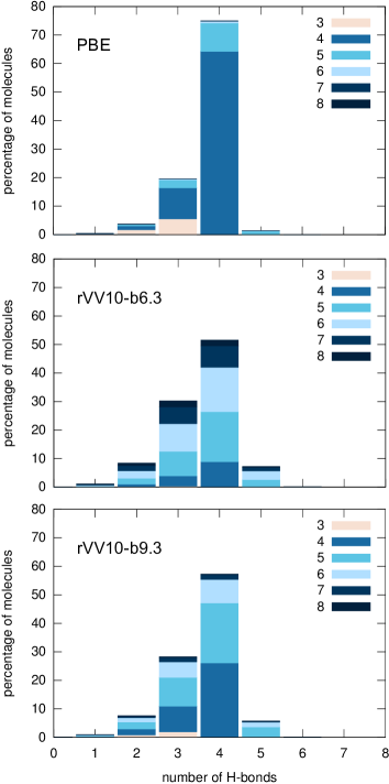
Figure 9: Distribution of water molecules with a given number of hydrogen bonds. The finer subdivisions within each bar, indicated by a color code, illustrate the associated distribution of coordination numbers. Since the same cutoff distance of 3.5 Å is used for defining the coordination number and the number of hydrogen bonds, the former cannot be smaller than the latter.

In Table 3, the percentage of molecules with a given number of hydrogen bonds is reported. In the PBE simulation, a large majority of molecules show four hydrogen bonds. Our result is in overall good agreement with a previous PBE study.Todorova et al. (2006) When van der Waals interactions are explicitly accounted for, the percentage of water molecules with either less or more than four hydrogen bonds increases. In particular, it can be seen from Table 3 that there are no significant differences between the percentage distributions achieved with rVV10-b6.3 and rVV10-b9.3. However, we here show that this structural descriptor overlooks important structural differences which relate to the occurrence of non-hydrogen bonded water molecules in the first coordination shell.

To highlight these structural differences, we illustrate the values given in Table 3 through a histogrammatic diagram in Fig. 9. Each bar, corresponding to the percentage of water molecules with a given number of hydrogen bonds, is now further analyzed according to the coordination number. The coordination number corresponds to the sum of all water molecules within the first coordination shell, either hydrogen-bonded or not. The first coordination shell is here defined by a cutoff distance of 3.5 Å, consistent with the adopted definition of hydrogen bond.Luzar and Chandler (1996); Schwegler, Galli, and Gygi (2000); Palmer et al. (2014) Let us focus on the most frequent situation corresponding to molecules with four hydrogen bonds. In the PBE simulation, most of these molecules are fourfold coordinated and only a small fraction of them is fivefold coordinated. The decomposition is very different for the rVV10 simulations, with the appearance of significant fractions of fivefold, sixfold, and sevenfold coordinated molecules. In particular, while the average number of molecules with four hydrogen bonds are similar in rVV10-b9.3 and rVV10-b6.3 (cf. Table 3), the finer subdivision clearly shows that the amount of highly coordinated molecules increases when going from rVV10-b9.3 to rVV10-b6.3.

We conclude our analysis of the hydrogen-bond network by focusing on the hydrogen bonds formed by the “interstitial” fifth water molecule within the first coordination shell of a central molecule. We focus on the most common situation in which a fifth molecule occurs in the coordination shell of a central molecule which is already engaged in four hydrogen bonds with the first four molecules. In such a situation, the fifth molecule could form a varying number of hydrogen bonds with the water molecules in the first coordination shell of the central one: either none, one, or two. In Table 4, we report the corresponding distributions for our simulations. In the PBE simulation, the fifth molecule generally forms at least one of such hydrogen bonds with a large probability (76%). At variance, in the rVV10 simulations, the most likely bonding corresponds to a fifth molecule without any of such hydrogen bonds. These results further confirm that the density increase in rVV10 simulations is not driven by the hydrogen-bond energy but rather to the enhanced stability of more compact water arrangements, as expected for the non-directional nature of the van der Waals interactions.

Table 4: Distribution of number of hydrogen bonds formed by a fifth molecule in the coordination shell of a central molecule which is already engaged in four hydrogen bonds with the first four molecules.

	Number of hydrogen bonds
	0	1	2
PBE	24%	55%	21%
rVV10-b6.3	60%	37%	3%
rVV10-b9.3	50%	44%	6%

V.5 Diffusion coefficient

To investigate the effect of van der Waals interactions on the mobility of water molecules, we focus on the self-diffusion coefficient. For a correct evaluation of the water self-diffusion coefficient, we perform a molecular dynamics simulation in the microcanonical ensemble (NVE). We use the rVV10-b9.3 functional and a simulation cell at a density of 1 g/cm³, which closely corresponds to the equilibrium density of liquid water for this functional. The average temperature in the simulation does not show any drift and averages to the value of 350 K. We collect data on an equilibrated simulation run of 25 ps.

The mean square displacement vs. time is determined as an average over all molecules and over trajectories with initial times separated by 100 fs. By virtue of Einstein’s relation, the calculated diffusion coefficient is derived from the slope of the mean square displacement and amounts to $D^{\textrm{sim}}=1.5\cdot 10^{-5}$ cm²/s.

Table 5: Self-diffusion coefficient $D^{\textrm{sim}}$ of liquid water as obtained in our NVE simulation based on the rVV10-b9.3 functional. The result of a previous PBE simulation performed at same density and temperature is also shown (Ref. Todorova et al., 2006). The diffusion coefficient obtained in the simulations are compared to reference values $D^{\textrm{ref}}$, which represent the experimental values for the cell size used in the simulation. For reference, we also give experimental values at 300 and 350 K as derived from Ref. 58.

	$T$ (K)	$D^{\textrm{sim}}$ (cm2/s)	$D^{\textrm{ref}}$ (cm2/s)
rVV10-b9.3	350	$1.5\cdot 10^{-5}$	$4.3\cdot 10^{-5}$
PBE (Ref. Todorova et al., 2006)	350	$0.47\cdot 10^{-5}$	$3.8\cdot 10^{-5}$
			$D^{\textrm{expt}}$ (cm2/s)
Expt.(extrapolated)	350		$6.2\cdot 10^{-5}$
Expt.	300		$2.4\cdot 10^{-5}$

The comparison of the calculated diffusion coefficient with experiment requires some care. Since the diffusion coefficient shows a strong dependence on temperature,Mills (1973) it is necessary to compare theoretical and experimental results achieved at the same temperature $T$. Based on experimental data in Ref. 58, we obtain an extrapolated experimental value of $D^{\textrm{expt.}}=6.2\cdot 10^{-5}$ cm²/s at 350 K, corresponding to the temperature in our simulation.

The comparison between theory and experiment is further affected by finite-size effects. To estimate these effects, we assume that the diffusion coefficient in the periodic cell underestimates the value corresponding to the infinite-size limit by: Dünweg and Kremer (1993); Yeh and Hummer (2004)

$$\Delta D=\frac{k_{\textrm{B}}T\xi}{6\pi\eta L}$$ (4)

where $k_{\textrm{B}}$ is the Boltzmann constant, $\xi=2.84$ a constant, $\eta$ the viscosity, and $L$ the side of the periodic cell. To take these finite-size effects into account we compare the calculated diffusion coefficient $D^{\textrm{sim}}$ with a reference value $D^{\textrm{ref}}$, which represent the experimental value for the temperature and cell size used in the simulation. For this purpose, we take for $\eta$ the experimental value of the viscosity at 350 K ($\eta^{\textrm{expt}}=3.12\cdot 10^{-4}$ Pa$\cdot$s) as extrapolated from the data in Ref. 65, and for $L$ the cubic cell side corresponding to 64 molecules at the experimental density ($L=12.4$ Å). For the conditions in our simulation, we thus obtain $\Delta D\approx 1.9\cdot 10^{-5}$ cm²/s and $D^{\textrm{ref}}=4.3\cdot 10^{-5}$ cm²/s. In Table 5, the diffusion coefficient $D^{\textrm{sim}}$ obtained from the molecular dynamics trajectory is directly compared with this reference value $D^{\textrm{ref}}$.

The comparison in Table 5 indicates that the diffusion coefficient obtained with the rVV10-b9.3 functional at 350 K ($D^{\textrm{sim}}=1.5\cdot 10^{-5}$ cm²/s) underestimates the reference value at the same temperature by a factor of about three. This discrepancy should be attributed to the cumulative effect resulting from the residual shortcomings of the adopted functional and the neglect of the quantum motion of the nuclei. However, the agreement is much better in case the calculated diffusion coefficient at 350 K is compared with a reference value derived from the experimental diffusion coefficient at 300 K ($1.8\cdot 10^{-5}$ cm²/s).

It is also instructive to compare the diffusion coefficients obtained with the rVV10-b9.3 functional with a previous PBE simulation at the same density and temperature.Todorova et al. (2006) The present simulation enhances the diffusion coefficient approximately by a factor of three, yielding an improved agreement with experiment. Indeed, the diffusion coefficient $D^{\textrm{sim}}$ obtained in the present rVV10-b9.3 simulation corresponds to 35% of the value of $D^{\textrm{ref}}$, whereas the $D^{\textrm{sim}}$ in the PBE simulation only reaches 12% of the respective reference value. Hence, the use of the present nonlocal van der Waals functional leads to an improved description of the water molecule mobility with respect to that achieved with the semilocal PBE functional.

VI Conclusions

We investigated the effect of explicitly including van der Waals interactions in ab initio molecular dynamics simulations of liquid water. Among the several available density functionals for treating van der Waals interactions, we adopted the rVV10 functional, which corresponds to a revised formSabatini, Gorni, and de Gironcoli (2013) of the formulation proposed by Vydrov and Van Voorhis.Vydrov and Van Voorhis (2010) This choice was motivated by the fact that the rVV10 functional allows for an evaluation of the total energy and the atomic forces at the same computational cost of standard semilocal functionals. Furthermore, once the phenomenological parameters in the rVV10 functional are set, the same theoretical scheme can be carried over to study aqueous solutions.

We first checked the accuracy of the nonlocal rVV10 functional in describing the water dimer and ice I${}_{\textrm{h}}$, finding energetic and structural properties in good agreement with both experimental and previous theoretical results. For these systems, the hydrogen-bond energy obtained with the rVV10 functional is in good agreement with both the experimental and the PBE result.

We then performed molecular dynamics simulations of liquid water in the $NpH$ statistical ensemble. In particular, we compared results obtained through simulations using PBE and rVV10 functionals. With the semilocal PBE functional, we obtained an equilibrium density of 0.87 g/cm³, significantly lower than the experimental density of 1 g/cm³, but in very good agreement with previous $NpT$ simulations based on the same functional.Schmidt et al. (2009) At variance, the rVV10 functional, in which the parameter $b$ is set to its original value (6.3, Ref. Sabatini, Gorni, and de Gironcoli, 2013), yields a density of 1.1 g/cm³. We found that the equilibrium density could be varied by modifying the parameter $b$. For $b=9.3$, we obtained an equilibrium density of 0.99 g/cm³, very close to the experimental value. Interestingly, we noticed that the use of rVV10-b9.3 also improved the local structure and the mobility of the water molecules. Indeed, the oxygen-oxygen radial distribution function in rVV10-b9.3 is in much better agreement with experiment than PBE. Furthermore, the average number of hydrogen bonds per molecule achieved with the rVV10-b9.3 functional (3.59) shows a closer agreement with the estimate derived from experimental data (3.58), than the corresponding numbers obtained with PBE (3.73) or rVV10-b6.3 (3.55).

The higher density achieved for liquid water with the nonlocal van der Waals functional indicates that the dispersion forces promote the role of non-directional interactions with respect to the semilocal functional in which the directionality of the hydrogen bonds dominates. The observed structural variations in liquid water thus arise from a different balance between non-directional and directional interactions.

In conclusion, our work demonstrates that the explicit treatment of van der Waals interactions through the rVV10 formulation considerably improves both the structural and the dynamical properties of liquid water with respect to the Perdew-Burke-Ernzerhof functional. This improvement is achieved without any significant computational overhead. Hence, the present theoretical framework should generally be preferred over the use of the Perdew-Burke-Ernzerhof functional in any application involving liquid water.