Optical analogy to quantum Fourier transform based on pseudorandom phase ensemble

Abstract

In this paper, we introduce an optical analogy to quantum Fourier tanformation based on a pseudorandom phase ensemble. The optical analogy also brings about exponential speedup over classical Fourier tanformation. Using the analogy, we demonstrate three classcial fields to realize Fourier transform similar to three quantum particles.

LABEL:FirstPage1

I Introduction

Quantum Fourier transform is the most important tool of quantum computation Nielsen , and one of the algorithms which can bring about exponential speedup. Shor’s algorithm, hidden subgroup problem and solving systems of linear equations all make use of quantum Fourier transform Montanaro . Quantum Fourier transform utilizes the superposition of quantum state, whereby the required time and space for computation can be notably reduced from $2^{n}$ to $n$. Hence, the implementation of quantum Fourier algorithm is crucial to exponential speedup in quantum computation Williams ; Deutsch .

A novel method to simulate quantum entanglement using classical fields modulated with pseudorandom phase sequences was introduced in Ref. Fu1 , which can realize tensor product in quantum computation and the representation of arbitrary quantum state Fu2 . At the same time, Ref. Fu3 also introduced a new concept, pseudorandom phase ensemble, to simulate a quantum ensemble. However, it is necessary to implement similar quantum Fourier transform algorithm to implement some current quantum algorithms. Therefore, in this paper, we, at first utilize this method to implement the simulation of quantum Fourier transform, then investigate the required computational resources, and at last take three kinds of fields as an example to verify this algorithm.

II Quantum Fourier transform

Generally, quantum Fourier transform takes as input a vector of complex numbers, $f(0),f(1)\ldots,f(N-1)$, and output a new vector of complex numbers $\tilde{f}(0),\tilde{f}(1)\ldots,\tilde{f}(N-1)$ as following:

$$\tilde{f}\left(k\right)=\frac{1}{\sqrt{N}}\sum\limits_{j=0}^{N-1}e^{\frac{2\pi i}{N}jk}f\left(j\right).$$ (1)

This calculation involves the additions and multiplications of $N=2^{n}$ complex numbers, leading to an increase of computational complexity with the increase of the number of vector components. Classically, the most effective algorithm, fast Fourier transform is in time $O(NlogN)$. On the contrary, the quantum Fourier transform can be defined as a unitary transformation on $n$ qubits Nielsen , which is:

$$\hat{F}\left|j\right\rangle=\frac{1}{\sqrt{2^{n}}}\sum\limits_{k=0}^{2^{n}-1}e^{\frac{2\pi i}{2^{n}}jk}\left|k\right\rangle.$$ (2)

Furthermore, the quantum Fourier transform of arbitrary state $\left|\Psi\right\rangle=C_{0}\left|0\right\rangle+\cdots+C_{2^{n}-1}\left|2^{n}-1\right\rangle$ can be expressed as:

$$\left|\Psi\right\rangle_{F} \equiv \hat{F}\left|\Psi\right\rangle=C_{0}\hat{F}\left|0\right\rangle+C_{1}\hat{F}\left|1\right\rangle+\cdots+C_{2^{n}-1}\hat{F}\left|2^{n}-1\right\rangle$$

$$= \frac{1}{\sqrt{2^{n}}}\sum\limits_{k=0}^{2^{n}-1}\left[C_{0}\omega^{0\ast k}+C_{1}\omega^{1\ast k}+\cdots+C_{2^{n}-1}\omega^{\left(2^{n}-1\right)\ast k}\right]\left|k\right\rangle,$$

where $\omega=e^{2\pi i/2^{n}}$. Then, we expand $\left|\Psi\right\rangle_{F}$ into:

$$\left|\Psi\right\rangle_{F}=\sum\limits_{j_{1}=0}^{1}\cdots\sum\limits_{j_{n}=0}^{1}D_{j_{n-1}\cdots j_{0}}\left|j_{n-1}\cdots j_{0}\right\rangle,$$ (4)

where the coefficients satisfy the following equation:

$$\left(\begin{array}[]{c}D_{0}\\ D_{1}\\ \vdots\\ D_{2^{n}-1}\end{array}\right)=\frac{1}{\sqrt{2^{n}}}\left(\begin{array}[]{cccc}1&1&\cdots&1\\ 1&\omega&\cdots&\omega^{2^{n}-1}\\ \vdots&\vdots&\ddots&\vdots\\ 1&\omega^{2^{n}-1}&\cdots&\omega^{\left(2^{n}-1\right)^{2}}\end{array}\right)\left(\begin{array}[]{c}C_{0}\\ C_{1}\\ \vdots\\ C_{2^{n}-1}\end{array}\right).$$ (5)

In quantum Fourier transform, after the Hadamard gate and controlled-phase gate, we can obtain the final state $\left|j\right\rangle=\left|j_{n-1}j_{n-2}\cdots j_{0}\right\rangle$ of quantum Fourier transform:

$$\hat{F}\left|j\right\rangle=\frac{1}{\sqrt{2^{n}}}\left(\left|1\right\rangle+e^{2\pi i0.j_{0}}\left|1\right\rangle\right)\left(\left|1\right\rangle+e^{2\pi i0.j_{1}j_{0}}\left|1\right\rangle\right)\cdots\left(\left|1\right\rangle+e^{2\pi i0.j_{n-1}j_{n-2}\cdots j_{0}}\left|1\right\rangle\right).$$ (6)

There are n Hadamard gates and $n(n-1)/2$ controlled-phase gates on n qubit registers, which means the quantum Fourier transform takes $O(n^{2})$ basic gate operations. Nevertheless, the quantum Fourier transform cannot output precise result of final states directly, but the probability of every state by repeated measurements, which can output the final result of Fourier transform at a certain accuracy Nielsen .

III Optical analogy to quantum Fourier transform

III.1 Simulation of quantum states based on pseudorandom phase ensemble

In Ref. Fu1 ; Fu2 ; Fu3 , a way to simulation of quantum states was introduced, which utilize the properties of pseudorandom sequence to modulate classical optical fields into different quantum states with different pseudorandom sequences. The formal product states for these fields can be a simulation to arbitrary quantum states in the pseudorandom phase ensemble model Fu3 . To further illustrate this method, the following is a brief introduction.

There are two orthogonal modes (polarization or transverse) of a classical field, which are denoted by $\left|0\right\rangle$ and $\left|1\right\rangle$, respectively. Thus, a qubit state $\left|\psi\right\rangle=\alpha\left|0\right\rangle+\beta\left|1\right\rangle$ can be expressed by the mode superposition, where $|\alpha|^{2}+|\beta|^{2}=1,(\alpha,\beta\in C)$. Obviously, all the mode superposition states span a Hilbert space. Choosing any $n$ PPSs from the set $\Xi=\{\lambda^{(0)},\lambda^{(1)},\ldots\lambda^{(M-1)}\}$ over $GF(p)$ to modulate $n$ classical fields, we can obtain the states expressed as follows:

$$\begin{array}[]{c}\left|\psi_{1}\right\rangle=e^{i\lambda^{(1)}}\left(\alpha_{1}\left|0\right\rangle+\beta_{1}\left|1\right\rangle\right),\\ \vdots\\ \left|\psi_{n}\right\rangle=e^{i\lambda^{(n)}}\left(\alpha_{n}\left|0\right\rangle+\beta_{n}\left|1\right\rangle\right).\end{array}$$ (7)

According to the properties of PPSs and Hilbert space, we can define the inner product of any two fields $\left|\psi_{a}\right\rangle$ and $\left|\psi_{b}\right\rangle$. We obtain the orthogonal property in our simulation,

$$\left\langle\psi_{a}\left|\psi_{b}\right.\right\rangle=\frac{1}{M}\sum\limits_{k=1}^{M}e^{i(\lambda_{k}^{(b)}-\lambda_{k}^{(a)})}(\alpha_{a}^{\ast}\alpha_{b}+\beta_{a}^{\ast}\beta_{b})=\left\{\begin{array}[]{c}1,a=b,\\ 0,a\neq b,\end{array}\right.$$ (8)

where $\lambda_{k}^{(a)},\lambda_{k}^{(b)}$ are the $k$-th units of $\lambda^{(a)}$ and $\lambda^{(b)}$, respectively. The orthogonal property supports the construction of the tensor product structure of the multiple states. A formal product state $\left|\Psi\right\rangle$ for the $n$ classical fields is defined as being a direct product of $\left|\psi_{i}\right\rangle,$

$$\left|\Psi\right\rangle=\left|\psi_{1}\right\rangle\otimes\left|\psi_{2}\right\rangle\otimes\cdots\otimes\left|\psi_{n}\right\rangle.$$ (9)

According to the definition, $n$ classical fields of Eq. (7) can be expressed as the following states:

$$\left|\Psi\right\rangle=e^{i\sum\nolimits_{j=1}^{n}\lambda^{\left(j\right)}}\left(\left|0\right\rangle+\left|1\right\rangle+\cdots+\left|2^{n}-1\right\rangle\right).$$ (10)

As mentioned in Fu1 ; Fu2 , a general form of $\left|\psi_{k}\right\rangle$ for $n$ fields can be constructed from Eq. (7) using a gate array model,

$$\left|\psi_{k}\right\rangle = \sum\limits_{i=1}^{n}\alpha_{k}^{\left(i\right)}e^{i\lambda^{\left(i\right)}}\left|0\right\rangle+\sum\limits_{j=1}^{n}\beta_{k}^{\left(j\right)}e^{i\lambda^{\left(j\right)}}\left|1\right\rangle$$

$$\equiv \tilde{\alpha}_{k}\left|0\right\rangle+\tilde{\beta}_{k}\left|1\right\rangle,$$

where $\tilde{\alpha}_{k}\equiv\sum\limits_{i=1}^{n}\alpha_{k}^{\left(i\right)}e^{i\lambda^{\left(i\right)}},\tilde{\beta}_{k}\equiv\sum\limits_{j=1}^{n}\beta_{k}^{\left(j\right)}e^{i\lambda^{\left(j\right)}}$. Then, the formal product state (9) can be written as

$$\left|\Psi\right\rangle=\left(\tilde{\alpha}_{1}\left|0\right\rangle+\tilde{\beta}_{1}\left|1\right\rangle\right)\otimes\cdots\otimes\left(\tilde{\alpha}_{n}\left|0\right\rangle+\tilde{\beta}_{n}\left|1\right\rangle\right).$$ (12)

Further, we can obtain each item of the superposition of $\left|\Psi\right\rangle$ as follows:

$$\begin{array}[]{c}C_{00\cdots 0}\left|00\cdots 0\right\rangle=\tilde{\alpha}_{1}\tilde{\alpha}_{2}\cdots\tilde{\alpha}_{n}\left|00\cdots 0\right\rangle,\\ C_{00\cdots 1}\left|00\cdots 1\right\rangle=\tilde{\alpha}_{1}\tilde{\alpha}_{2}\cdots\tilde{\beta}_{n}\left|00\cdots 1\right\rangle,\\ \vdots\\ C_{11\cdots 1}\left|11\cdots 1\right\rangle=\tilde{\beta}_{1}\tilde{\beta}_{2}\cdots\tilde{\beta}_{n}\left|11\cdots 1\right\rangle.\end{array}$$ (13)

According to the closure property Fu1 , the phase sequences $\lambda^{\left(j\right)}$ of $C_{i_{1}i_{2}\cdots i_{n}}$ remain in the set $\Xi$, which means $C_{i_{1}i_{2}\cdots i_{n}}=\sum\limits_{j=0}^{M-1}C_{i_{1}i_{2}\cdots i_{n}}^{\left(j\right)}e^{i\lambda^{\left(j\right)}}$. Therefore, we obtain the formal product state $\left|\Psi\right\rangle$ spans a Hilbert space with the basis $\left\{\left.e^{i\lambda^{\left(j\right)}}\left|i_{1}i_{2}\cdots i_{n}\right\rangle\right|\lambda^{\left(j\right)}\in\Xi,j=0\cdots M-1,i_{n}=0or1\right\}$ and can be expressed as follows:

$$\left|\Psi\right\rangle=\sum\limits_{i_{1}=0}^{1}\cdots\sum\limits_{i_{n}=0}^{1}\left[\sum\limits_{j=0}^{M-1}C_{i_{1}i_{2}\cdots i_{n}}^{\left(j\right)}e^{i\lambda^{\left(j\right)}}\left|i_{1}i_{2}\cdots i_{n}\right\rangle\right],$$ (14)

where $C_{i_{1}i_{2}\cdots i_{n}}^{\left(j\right)}$ denotes a total of $M2^{n}$ coefficients.

Ref. Fu3 further proposed the ensemble-averaged reduced states in ensemble model, which utilize the closure and balance property of pseudorandom phase sequence to remove some terms in the formal product states after ensemble averaging, whereby the required arbitrary quantum states can be obtained, including quantum entanglement states.

III.2 Algorithm for the optical analogy

Considering a quantum state $\left|\Psi\right\rangle$ expressed by $n$ classical fields, according to the equation (14), we obtain its formal product states as following:

$$\left|\Psi\right\rangle=\sum\limits_{i_{1}=0}^{1}\cdots\sum\limits_{i_{n}=0}^{1}C_{i_{1}i_{2}\cdots i_{n}}\left|i_{1}i_{2}\cdots i_{n}\right\rangle,$$ (15)

where $C_{i_{1}i_{2}\cdots i_{N}}$ is the same as that in Eq. (14). After quantum Fourier transform, this state involves into

$$\left|\Psi\right\rangle_{F}=\hat{F}\left|\Psi\right\rangle,$$ (16)

where

$$\left|\Psi\right\rangle_{F}=\sum\limits_{j_{1}=0}^{1}\cdots\sum\limits_{j_{n}=0}^{1}D_{j_{1}j_{2}\cdots j_{n}}\left|j_{1}j_{2}\cdots j_{n}\right\rangle.$$ (17)

According to the definition Eq. (1), the relation between the coefficients $C_{i_{1}i_{2}\cdots i_{n}}$ and $D_{j_{1}j_{2}\cdots j_{n}}$ of these two states have to be satisfied as Eq. (5). To obtain the relation between these coefficient, we design the following algortithm:

(1) Selected a basis state $\left|j_{1}j_{2}\cdots j_{n}\right\rangle$ of $\left|\Psi\right\rangle_{F}$;

(2) Apply the following controlled-phase transformation on every field of $\left|\Psi\right\rangle$ according to the specific value of bits in the selected basis state:

$$\left\{\begin{array}[]{c}\left|\psi_{1}\right\rangle=\tilde{\alpha}_{1}\left|0\right\rangle+\tilde{\beta}_{1}\left|1\right\rangle\\ \left|\psi_{2}\right\rangle=\tilde{\alpha}_{2}\left|0\right\rangle+\omega^{j_{1}\ast 2^{n-2}}\tilde{\beta}_{2}\left|1\right\rangle\\ \left|\psi_{3}\right\rangle=\tilde{\alpha}_{3}\left|0\right\rangle+\omega^{j_{2}\ast 2^{n-2}+j_{1}\ast 2^{n-3}}\tilde{\beta}_{3}\left|1\right\rangle\\ \cdots\\ \left|\psi_{n}\right\rangle=\tilde{\alpha}_{n}\left|0\right\rangle+\omega^{j_{n-1}\ast 2^{n-2}+j_{n-2}\ast 2^{n-3}+\cdots+j_{1}\ast 1}\tilde{\beta}_{n}\left|1\right\rangle\end{array}\right.$$ (18)

(3) Apply Hadamard gate on these fields, after which we obtain:

$$\left\{\begin{array}[]{c}\left|\psi_{1}\right\rangle=\left(\tilde{\alpha}_{1}+\tilde{\beta}_{1}\right)\left|0\right\rangle+\left(\tilde{\alpha}_{1}-\tilde{\beta}_{1}\right)\left|1\right\rangle\\ \left|\psi_{2}\right\rangle=\left(\tilde{\alpha}_{2}+\omega^{j_{1}\ast 2^{n-2}}\tilde{\beta}_{2}\right)\left|0\right\rangle+\left(\tilde{\alpha}_{2}-\omega^{j_{1}\ast 2^{n-2}}\tilde{\beta}_{2}\right)\left|1\right\rangle\\ \left|\psi_{3}\right\rangle=\left(\tilde{\alpha}_{3}+\omega^{j_{2}\ast 2^{n-2}+j_{1}\ast 2^{n-3}}\tilde{\beta}_{3}\right)\left|0\right\rangle+\left(\tilde{\alpha}_{3}-\omega^{j_{2}\ast 2^{n-2}+j_{1}\ast 2^{n-3}}\tilde{\beta}_{3}\right)\left|1\right\rangle\\ \cdots\\ \left|\psi_{n}\right\rangle=\left(\tilde{\alpha}_{n}+\omega^{j_{n-1}\ast 2^{n-2}+j_{n-2}\ast 2^{n-3}+\cdots+j_{1}}\tilde{\beta}_{n}\right)\tilde{\alpha}_{n}\left|0\right\rangle+\left(\tilde{\alpha}_{n}-\omega^{j_{n-1}\ast 2^{n-2}+j_{n-2}\ast 2^{n-3}+\cdots+j_{1}}\tilde{\beta}_{n}\right)\left|1\right\rangle\end{array}\right.$$ (19)

(4) Apply the mode selection gate on these fields according to the specific values in $\left|j_{1}j_{2}\cdots j_{n}\right\rangle$, after which the mode of every field is identical to the corresponding value in $\left|j_{1}j_{2}\cdots j_{n}\right\rangle$, e.g., if $j_{1}=0$, $\left|\psi_{1}\right\rangle\rightarrow\left(\tilde{\alpha}_{1}+\tilde{\beta}_{1}\right)\left|0\right\rangle$, while if $j_{1}=1$, $\left|\psi_{1}\right\rangle\rightarrow\left(\tilde{\alpha}_{1}-\tilde{\beta}_{1}\right)\left|1\right\rangle$;

(5) Apply mode detection on these fields and obtain the M matrix. Then we can obtain the corresponding coefficient $D_{j_{n}j_{n-1}\cdots j_{1}}$ using the method in Ref. Fu2 .

The above algorithm can be summarized as the following block diagram in Fig. 1.

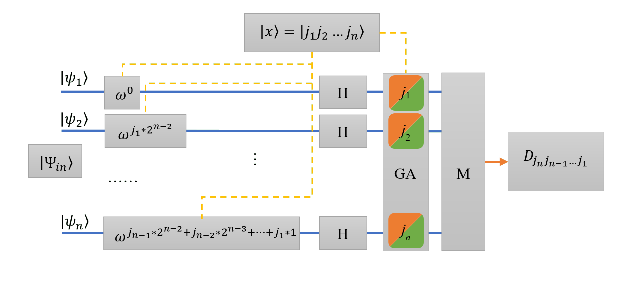
Figure 1: The algorithm diagram of optical analogy to quantum Fourier transformation.

At last, we can analysis the computational complexity: there are $n$ fields in $\left|\Psi\right\rangle$ after $n$ controlled-phase gates, $n$ Hadamard gates, $n$ mode selection operations and finally $n^{2}$ correlation detection in mode detection. Hence, the total number of operations is in $O(n^{2})$, which is the same as that in quantum Fourier transform. However, the result we obtain is with certainty but not with probability like the case in quantum Fourier transform.

III.3 The equivalence of ensemble-averaged reduced states in optical analogy algorithm

In pseudorandom phase ensemble, we utilize the characteristic of pseudorandom phase sequence to define the ensemble-averaged reduced state Fu3 . The balance property of pseudorandom phase sequences Fu1 : with the exception of $\lambda^{\left(0\right)}$, any sequence of the set $\Omega$ satisfies

$$\sum\limits_{k=1}^{M}e^{i\theta}e^{i\lambda_{k}^{\left(j\right)}}=\sum\limits_{k=1}^{M}e^{i\left(\theta+\lambda_{k}^{\left(j\right)}\right)}=0,\forall\theta\in\mathbb{R}$$ (20)

where $\lambda_{k}^{\left(j\right)}$ is the $k$-th phase unit in pseudorandom sequence $\lambda^{\left(j\right)}$. Due to this property, several terms of the formal product state can be reduced under ensemble averaging, enabling us to utilize classical fields to simulation arbitrary quantum states. According to Ref. Fu3 , the reduced state can be defined as

$$\left|\tilde{\Psi}\right\rangle\equiv\sum\limits_{k=1}^{M}e^{-i\lambda^{\left(S\right)}}\left|\Psi\right\rangle$$ (21)

where $\lambda^{\left(S\right)}=\sum\nolimits_{k=1}^{n}\lambda^{(k)}$, which is the sum of all phase sequences of classical fields.

Then, we discuss about the quantum Fourier transform of ensemble-averaged reduced states. From equation (5), we obtain the coefficients of quantum Fourier transform satisfies

$$\begin{array}[]{c}D_{00\cdots 0}=C_{00\cdots 0}+C_{00\cdots 1}+\cdots+C_{11\cdots 1}\\ D_{00\cdots 1}=C_{00\cdots 0}+\omega C_{00\cdots 1}+\cdots+\omega^{\left(2^{n}-1\right)}C_{11\cdots 1}\\ \cdots\\ D_{11\cdots 0}=C_{00\cdots 0}+\omega^{\left(2^{n}-2\right)}C_{00\cdots 1}+\cdots+\omega^{\left(2^{n}-2\right)\left(2^{n}-1\right)}C_{11\cdots 1}\\ D_{11\cdots 1}=C_{00\cdots 0}+\omega^{\left(2^{n}-1\right)}C_{00\cdots 1}+\cdots+\omega^{\left(2^{n}-1\right)^{2}}C_{11\cdots 1}\end{array}$$ (22)

In these equations, the combinations of $\omega$ and $C_{i_{1}i_{2}\cdots i_{n}}$ satisfy the following relations:

$$\omega^{k}C_{i_{1}i_{2}\cdots i_{n}}=\sum\limits_{j=1}^{M}C_{i_{1}i_{2}\cdots i_{n}}^{\left(j\right)}e^{i\left[\lambda^{\left(j\right)}+2\pi k/2^{n}\right]}$$ (23)

Obviously, these terms also satisfy the balance property of pseudorandom sequence. Hence, the ensemble-averaged reduced states can also be used in the states after quantum Fourier transform. Then, we can obtain the Fourier transform:

$$\left|\tilde{\Psi}\right\rangle_{F}\equiv\sum\limits_{k=1}^{M}e^{-i\lambda^{\left(S\right)}}\left|\Psi\right\rangle_{F}=\hat{F}\sum\limits_{k=1}^{M}e^{-i\lambda^{\left(S\right)}}\left|\Psi\right\rangle=\hat{F}\left|\tilde{\Psi}\right\rangle$$ (24)

At last, we show the equivalence of ensemble-averaged reduced states in quantum Fourier transform.

IV Optical analogy to quantum Fourier transform for three particles

According to Ref. Fu2 , three pseudorandom phase sequences $\lambda^{\left(i\right)}\left(i=1,2,3\right)$ are required to implement the simulation of the quantum states consisting of three particles. Modulated with these phase sequence, three classical optical fields can be expressed as following:

$$\left\{\begin{array}[]{c}\left|\psi_{1}\right\rangle=e^{i\lambda^{\left(1\right)}}\left(\left|0\right\rangle+\left|1\right\rangle\right)\\ \left|\psi_{2}\right\rangle=e^{i\lambda^{\left(2\right)}}\left(\left|0\right\rangle+\left|1\right\rangle\right)\\ \left|\psi_{3}\right\rangle=e^{i\lambda^{\left(3\right)}}\left(\left|0\right\rangle+\left|1\right\rangle\right)\end{array}\right.$$ (25)

After proper gate array operation Fu3 , we can obtain arbitrary quantum states which can be expressed as following:

$$\left\{\begin{array}[]{c}\left|\psi_{1}\right\rangle=\tilde{\alpha}_{1}\left|0\right\rangle+\tilde{\beta}_{1}\left|1\right\rangle\\ \left|\psi_{2}\right\rangle=\tilde{\alpha}_{2}\left|0\right\rangle+\tilde{\beta}_{2}\left|1\right\rangle\\ \left|\psi_{3}\right\rangle=\tilde{\alpha}_{3}\left|0\right\rangle+\tilde{\beta}_{3}\left|1\right\rangle\end{array}\right.$$ (26)

According to the algorithm in Sec. III.2, we obtain:

(1) Apply controlled-phase gates on three classical fields respectively:

$$\left\{\begin{array}[]{c}\left|\psi_{1}\right\rangle=\tilde{\alpha}_{1}\left|0\right\rangle+\tilde{\beta}_{1}\left|1\right\rangle\\ \left|\psi_{2}\right\rangle=\tilde{\alpha}_{2}\left|0\right\rangle+\omega^{j_{1}\ast 2}\tilde{\beta}_{2}\left|1\right\rangle\\ \left|\psi_{3}\right\rangle=\tilde{\alpha}_{3}\left|0\right\rangle+\omega^{j_{2}\ast 2+j_{1}\ast 1}\tilde{\beta}_{3}\left|1\right\rangle\end{array}\right.$$ (27)

where $\omega=e^{2\pi i/8}$.

(2) Hadamard transformation

$$\left\{\begin{array}[]{c}\left|\psi_{1}\right\rangle=\left(\tilde{\alpha}_{1}+\tilde{\beta}_{1}\right)\left|0\right\rangle+\left(\tilde{\alpha}_{1}-\tilde{\beta}_{1}\right)\left|1\right\rangle\\ \left|\psi_{2}\right\rangle=\left(\tilde{\alpha}_{2}+\omega^{j_{1}\ast 2}\tilde{\beta}_{2}\right)\left|0\right\rangle+\left(\tilde{\alpha}_{2}-\omega^{j_{1}\ast 2}\tilde{\beta}_{2}\right)\left|1\right\rangle\\ \left|\psi_{3}\right\rangle=\left(\tilde{\alpha}_{3}+\omega^{j_{2}\ast 2+j_{1}\ast 1}\tilde{\beta}_{3}\right)\left|0\right\rangle+\left(\tilde{\alpha}_{3}-\omega^{j_{2}\ast 2+j_{1}\ast 1}\tilde{\beta}_{3}\right)\left|1\right\rangle\end{array}\right.$$ (28)

(3) Calculate coefficients

(3.1) When $\left|j_{1}j_{2}j_{3}\right\rangle=\left|000\right\rangle$ and $\left|j_{1}j_{2}j_{3}\right\rangle=\left|001\right\rangle$,

$$\left\{\begin{array}[]{c}\left|\psi_{1}\right\rangle=\tilde{\alpha}_{1}\left|0\right\rangle+\tilde{\beta}_{1}\left|1\right\rangle\\ \left|\psi_{2}\right\rangle=\tilde{\alpha}_{2}\left|0\right\rangle+\omega^{0\ast 2}\tilde{\beta}_{2}\left|1\right\rangle\\ \left|\psi_{3}\right\rangle=\tilde{\alpha}_{3}\left|0\right\rangle+\omega^{0\ast 2+0\ast 1}\tilde{\beta}_{3}\left|1\right\rangle\end{array}\right.\rightarrow\left\{\begin{array}[]{c}\left|\psi_{1}\right\rangle=\left(\tilde{\alpha}_{1}+\tilde{\beta}_{1}\right)\left|0\right\rangle+\left(\tilde{\alpha}_{1}-\tilde{\beta}_{1}\right)\left|1\right\rangle\\ \left|\psi_{2}\right\rangle=\left(\tilde{\alpha}_{2}+\tilde{\beta}_{2}\right)\left|0\right\rangle+\left(\tilde{\alpha}_{2}-\tilde{\beta}_{2}\right)\left|1\right\rangle\\ \left|\psi_{3}\right\rangle=\left(\tilde{\alpha}_{3}+\tilde{\beta}_{3}\right)\left|0\right\rangle+\left(\tilde{\alpha}_{3}-\tilde{\beta}_{3}\right)\left|1\right\rangle\end{array}\right..$$ (29)

Then obtain the corresponding coefficients $D_{000}$ and $D_{100}$:

$$D_{000} = \left(\tilde{\alpha}_{1}+\tilde{\beta}_{1}\right)\left(\tilde{\alpha}_{2}+\tilde{\beta}_{2}\right)\left(\tilde{\alpha}_{3}+\tilde{\beta}_{3}\right)$$

$$= C_{000}+C_{001}+C_{010}+C_{011}+C_{100}+C_{101}+C_{110}+C_{111},$$

$$D_{100} = \left(\tilde{\alpha}_{1}+\tilde{\beta}_{1}\right)\left(\tilde{\alpha}_{2}+\tilde{\beta}_{2}\right)\left(\tilde{\alpha}_{3}-\tilde{\beta}_{3}\right)$$

$$= C_{000}-C_{001}+C_{010}-C_{011}+C_{100}-C_{101}+C_{110}-C_{111}.$$

(3.2) When $\left|j_{1}j_{2}j_{3}\right\rangle=\left|010\right\rangle$ and $\left|j_{1}j_{2}j_{3}\right\rangle=\left|011\right\rangle$,

$$\left\{\begin{array}[]{c}\left|\psi_{1}\right\rangle=\tilde{\alpha}_{1}\left|0\right\rangle+\tilde{\beta}_{1}\left|1\right\rangle\\ \left|\psi_{2}\right\rangle=\tilde{\alpha}_{2}\left|0\right\rangle+\omega^{0\ast 2}\tilde{\beta}_{2}\left|1\right\rangle\\ \left|\psi_{3}\right\rangle=\tilde{\alpha}_{3}\left|0\right\rangle+\omega^{1\ast 2+0\ast 1}\tilde{\beta}_{3}\left|1\right\rangle\end{array}\right.\rightarrow\left\{\begin{array}[]{c}\left|\psi_{1}\right\rangle=\left(\tilde{\alpha}_{1}+\tilde{\beta}_{1}\right)\left|0\right\rangle+\left(\tilde{\alpha}_{1}-\tilde{\beta}_{1}\right)\left|1\right\rangle\\ \left|\psi_{2}\right\rangle=\left(\tilde{\alpha}_{2}+\tilde{\beta}_{2}\right)\left|0\right\rangle+\left(\tilde{\alpha}_{2}-\tilde{\beta}_{2}\right)\left|1\right\rangle\\ \left|\psi_{3}\right\rangle=\left(\tilde{\alpha}_{3}+\omega^{2}\tilde{\beta}_{3}\right)\left|0\right\rangle+\left(\tilde{\alpha}_{3}-\omega^{2}\tilde{\beta}_{3}\right)\left|1\right\rangle\end{array}\right..$$ (32)

Then obtain the corresponding coefficients $D_{010}$ and $D_{110}$:

$$D_{010} = \left(\tilde{\alpha}_{1}+\tilde{\beta}_{1}\right)\left(\tilde{\alpha}_{2}-\tilde{\beta}_{2}\right)\left(\tilde{\alpha}_{3}+\omega^{2}\tilde{\beta}_{3}\right)$$

$$= C_{000}+\omega^{2}C_{001}-C_{010}-\omega^{2}C_{011}+C_{100}+\omega^{2}C_{101}-C_{110}-\omega^{2}C_{111},$$

$$D_{110} = \left(\tilde{\alpha}_{1}+\tilde{\beta}_{1}\right)\left(\tilde{\alpha}_{2}-\tilde{\beta}_{2}\right)\left(\tilde{\alpha}_{3}-\omega^{2}\tilde{\beta}_{3}\right)$$

$$= C_{000}-\omega^{2}C_{001}-C_{010}+\omega^{2}C_{011}+C_{100}-\omega^{2}C_{101}-C_{110}+\omega^{2}C_{111}.$$

(3.3) When $\left|j_{1}j_{2}j_{3}\right\rangle=\left|100\right\rangle$ and $\left|j_{1}j_{2}j_{3}\right\rangle=\left|101\right\rangle$,

$$\left\{\begin{array}[]{c}\left|\psi_{1}\right\rangle=\tilde{\alpha}_{1}\left|0\right\rangle+\tilde{\beta}_{1}\left|1\right\rangle\\ \left|\psi_{2}\right\rangle=\tilde{\alpha}_{2}\left|0\right\rangle+\omega^{1\ast 2}\tilde{\beta}_{2}\left|1\right\rangle\\ \left|\psi_{3}\right\rangle=\tilde{\alpha}_{3}\left|0\right\rangle+\omega^{0\ast 2+1\ast 1}\tilde{\beta}_{3}\left|1\right\rangle\end{array}\right.\rightarrow\left\{\begin{array}[]{c}\left|\psi_{1}\right\rangle=\left(\tilde{\alpha}_{1}+\tilde{\beta}_{1}\right)\left|0\right\rangle+\left(\tilde{\alpha}_{1}-\tilde{\beta}_{1}\right)\left|1\right\rangle\\ \left|\psi_{2}\right\rangle=\left(\tilde{\alpha}_{2}+\omega^{2}\tilde{\beta}_{2}\right)\left|0\right\rangle+\left(\tilde{\alpha}_{2}-\omega^{2}\tilde{\beta}_{2}\right)\left|1\right\rangle\\ \left|\psi_{3}\right\rangle=\left(\tilde{\alpha}_{3}+\omega\tilde{\beta}_{3}\right)\left|0\right\rangle+\left(\tilde{\alpha}_{3}-\omega\tilde{\beta}_{3}\right)\left|1\right\rangle\end{array}\right..$$ (35)

Then obtain the corresponding coefficients $D_{001}$ and $D_{101}$:

$$D_{001} = \left(\tilde{\alpha}_{1}-\tilde{\beta}_{1}\right)\left(\tilde{\alpha}_{2}+\omega^{2}\tilde{\beta}_{2}\right)\left(\tilde{\alpha}_{3}+\omega\tilde{\beta}_{3}\right)$$

$$= C_{000}+\omega C_{001}+\omega^{2}C_{010}+\omega^{3}C_{011}-C_{100}-\omega C_{101}-\omega^{2}C_{110}-\omega^{3}C_{111},$$

$$D_{101} = \left(\tilde{\alpha}_{1}-\tilde{\beta}_{1}\right)\left(\tilde{\alpha}_{2}+\omega^{2}\tilde{\beta}_{2}\right)\left(\tilde{\alpha}_{3}-\omega\tilde{\beta}_{3}\right)$$

$$= C_{000}-\omega C_{001}+\omega^{2}C_{010}-\omega^{3}C_{011}-C_{100}+\omega C_{101}-\omega^{2}C_{110}+\omega^{3}C_{111}.$$

(3.4) When $\left|j_{1}j_{2}j_{3}\right\rangle=\left|110\right\rangle$ and $\left|j_{1}j_{2}j_{3}\right\rangle=\left|111\right\rangle$,

$$\left\{\begin{array}[]{c}\left|\psi_{1}\right\rangle=\tilde{\alpha}_{1}\left|0\right\rangle+\tilde{\beta}_{1}\left|1\right\rangle\\ \left|\psi_{2}\right\rangle=\tilde{\alpha}_{2}\left|0\right\rangle+\omega^{1\ast 2}\tilde{\beta}_{2}\left|1\right\rangle\\ \left|\psi_{3}\right\rangle=\tilde{\alpha}_{3}\left|0\right\rangle+\omega^{1\ast 2+1\ast 1}\tilde{\beta}_{3}\left|1\right\rangle\end{array}\right.\rightarrow\left\{\begin{array}[]{c}\left|\psi_{1}\right\rangle=\left(\tilde{\alpha}_{1}+\tilde{\beta}_{1}\right)\left|0\right\rangle+\left(\tilde{\alpha}_{1}-\tilde{\beta}_{1}\right)\left|1\right\rangle\\ \left|\psi_{2}\right\rangle=\left(\tilde{\alpha}_{2}+\omega^{2}\tilde{\beta}_{2}\right)\left|0\right\rangle+\left(\tilde{\alpha}_{2}-\omega^{2}\tilde{\beta}_{2}\right)\left|1\right\rangle\\ \left|\psi_{3}\right\rangle=\left(\tilde{\alpha}_{3}+\omega^{3}\tilde{\beta}_{3}\right)\left|0\right\rangle+\left(\tilde{\alpha}_{3}-\omega^{3}\tilde{\beta}_{3}\right)\left|1\right\rangle\end{array}\right..$$ (38)

Then obtain the corresponding coefficients $D_{011}$ and $D_{111}$:

$$D_{011} = \left(\tilde{\alpha}_{1}-\tilde{\beta}_{1}\right)\left(\tilde{\alpha}_{2}-\omega^{2}\tilde{\beta}_{2}\right)\left(\tilde{\alpha}_{3}+\omega^{3}\tilde{\beta}_{3}\right)$$

$$= C_{000}+\omega^{3}C_{001}-\omega^{2}C_{010}-\omega^{5}C_{011}-C_{100}-\omega^{3}C_{101}+\omega^{2}C_{110}+\omega^{5}C_{111},$$

$$D_{110} = \left(\tilde{\alpha}_{1}-\tilde{\beta}_{1}\right)\left(\tilde{\alpha}_{2}-\tilde{\beta}_{2}\right)\left(\tilde{\alpha}_{3}-\omega^{2}\tilde{\beta}_{3}\right)$$

$$= C_{000}-\omega^{3}C_{001}-\omega^{2}C_{010}+\omega^{5}C_{011}-C_{100}+\omega^{3}C_{101}+\omega^{2}C_{110}-\omega^{5}C_{111}.$$

At last, we obtain the transform matrix of all coefficients as following:

$$\left(\begin{array}[]{c}D_{000}\\ D_{001}\\ D_{010}\\ D_{011}\\ D_{100}\\ D_{101}\\ D_{110}\\ D_{111}\end{array}\right)=\left(\begin{array}[]{cccccccc}1&1&1&1&1&1&1&1\\ 1&\omega&\omega^{2}&\omega^{3}&-1&-\omega&-\omega^{2}&-\omega^{3}\\ 1&\omega^{2}&-1&-\omega^{2}&1&\omega^{2}&-1&\omega^{2}\\ 1&\omega^{3}&-\omega^{2}&\omega&-1&-\omega^{3}&\omega^{2}&-\omega\\ 1&-1&1&-1&1&-1&1&-1\\ 1&-\omega&\omega^{2}&-\omega^{3}&-1&\omega&-\omega^{2}&\omega^{3}\\ 1&-\omega^{2}&-1&\omega^{2}&1&-\omega^{2}&-1&\omega^{2}\\ 1&-\omega^{3}&-\omega^{2}&-\omega&-1&\omega^{3}&\omega^{2}&\omega\end{array}\right)\left(\begin{array}[]{c}C_{000}\\ C_{001}\\ C_{010}\\ C_{011}\\ C_{100}\\ C_{101}\\ C_{110}\\ C_{111}\end{array}\right)$$ (41)

We will utilize the above algorithm to apply quantum Fourier transform on several kinds of states in the following:

(1) Product state

In quantum mechanics, the product state of three particles is $\left|\Psi\right\rangle=\frac{1}{\sqrt{8}}\left(\left|000\right\rangle+\left|001\right\rangle+\cdots+\left|111\right\rangle\right)$. We can expressed these three fields as equation (25), except for normalization constant. In Ref. [6], the formal product state of this state can be expressed as:

$$\left|\Psi\right\rangle=\left|\psi_{1}\right\rangle\otimes\left|\psi_{2}\right\rangle\otimes\left|\psi_{3}\right\rangle=e^{i\left(\lambda^{\left(1\right)}+\lambda^{\left(2\right)}+\lambda^{\left(3\right)}\right)}\left(\left|000\right\rangle+\left|001\right\rangle+\cdots+\left|111\right\rangle\right)$$ (42)

Except for normalization constant and overall phase factor, that is, the sum of three pseudorandom sequence, there is not difference between this state and the product state of three particles. From Ref. Fu2 ; Fu3 , utilizing the concept of pseudorandom phase ensemble and the properties of pseudorandom sequence, we obtain the ensemble-averaged reduced state:

$$\left|\tilde{\Psi}\right\rangle=\left|000\right\rangle+\left|001\right\rangle+\cdots+\left|111\right\rangle$$ (43)

Using the above algorithm, we can easily obtain the coefficients of the Fourier transform of this state, $D_{000}=C_{000}+C_{001}+\cdots+C_{111}=8e^{i\left(\lambda^{\left(1\right)}+\lambda^{\left(2\right)}+\lambda^{\left(3\right)}\right)}$, while the other terms is 0. Then we obtain:

$$\left|\tilde{\Psi}\right\rangle_{F}=8\left|000\right\rangle$$ (44)

which is identical to the quantum Fourier transform, except for the normalization constant.

(2) GHZ state

In quantum mechanics, GHZ state is biggest entanglement state in the system of the three particles. This state is of great importance since it can verify the entanglement criterion in the correlation measurement of quantum entanglement. From Ref. Fu2 , we can obtain the following form of three fields by proper transformation:

$$\left\{\begin{array}[]{c}\left|\psi_{1}\right\rangle=\tilde{\alpha}_{1}\left|0\right\rangle+\tilde{\beta}_{1}\left|1\right\rangle=e^{i\lambda^{\left(1\right)}}\left|0\right\rangle+e^{i\lambda^{\left(2\right)}}\left|1\right\rangle\\ \left|\psi_{2}\right\rangle=\tilde{\alpha}_{2}\left|0\right\rangle+\tilde{\beta}_{2}\left|1\right\rangle=e^{i\lambda^{\left(2\right)}}\left|0\right\rangle+e^{i\lambda^{\left(3\right)}}\left|1\right\rangle\\ \left|\psi_{3}\right\rangle=\tilde{\alpha}_{3}\left|0\right\rangle+\tilde{\beta}_{3}\left|1\right\rangle=e^{i\lambda^{\left(3\right)}}\left|0\right\rangle+e^{i\lambda^{\left(1\right)}}\left|1\right\rangle\end{array}\right.$$ (45)

The formal product state of these three fields can be expressed as:

$$\left|\Psi\right\rangle = \left|\psi_{1}\right\rangle\otimes\left|\psi_{2}\right\rangle\otimes\left|\psi_{3}\right\rangle=e^{i\left(\lambda^{\left(1\right)}+\lambda^{\left(2\right)}+\lambda^{\left(3\right)}\right)}\left[\left|000\right\rangle+\left|111\right\rangle+e^{i\left(\lambda^{\left(1\right)}-\lambda^{\left(3\right)}\right)}\left|001\right\rangle\right.$$

$$+e^{i\left(\lambda^{\left(3\right)}-\lambda^{\left(2\right)}\right)}\left|010\right\rangle+e^{i\left(\lambda^{\left(1\right)}-\lambda^{\left(2\right)}\right)}\left|011\right\rangle+e^{i\left(\lambda^{\left(2\right)}-\lambda^{\left(1\right)}\right)}\left|100\right\rangle$$

$$\left.+e^{i\left(\lambda^{\left(2\right)}-\lambda^{\left(3\right)}\right)}\left|101\right\rangle+e^{i\left(\lambda^{\left(3\right)}-\lambda^{\left(1\right)}\right)}\left|110\right\rangle\right]$$

From Ref. Fu2 ; Fu3 , utilizing the concept of pseudorandom phase ensemble and the properties of pseudorandom sequence, we obtain the ensemble-averaged reduced state:

$$\left|\tilde{\Psi}\right\rangle=\left|000\right\rangle+\left|111\right\rangle$$ (47)

Similarly, except for normalization constant and overall phase factor, the state is identical to GHZ state.

Using the above algorithm, we can easily obtain the coefficients of the Fourier transform of this state respectively:

$$D_{000} = \left(\tilde{\alpha}_{1}+\tilde{\beta}_{1}\right)\left(\tilde{\alpha}_{2}+\tilde{\beta}_{2}\right)\left(\tilde{\alpha}_{3}+\tilde{\beta}_{3}\right)=2e^{i\left(\lambda^{\left(1\right)}+\lambda^{\left(2\right)}+\lambda^{\left(3\right)}\right)}+e^{i\left(2\lambda^{\left(1\right)}+\lambda^{\left(2\right)}\right)}+e^{i\left(2\lambda^{\left(1\right)}+\lambda^{\left(3\right)}\right)}$$ (48)

$$+e^{i\left(2\lambda^{\left(2\right)}+\lambda^{\left(1\right)}\right)}+e^{i\left(2\lambda^{\left(2\right)}+\lambda^{\left(3\right)}\right)}+e^{i\left(2\lambda^{\left(3\right)}+\lambda^{\left(1\right)}\right)}+e^{i\left(2\lambda^{\left(3\right)}+\lambda^{\left(2\right)}\right)},$$

$$D_{001} = \left(\tilde{\alpha}_{1}-\tilde{\beta}_{1}\right)\left(\tilde{\alpha}_{2}+\omega^{2}\tilde{\beta}_{2}\right)\left(\tilde{\alpha}_{3}+\omega\tilde{\beta}_{3}\right)=\left(1-\omega^{3}\right)e^{i\left(\lambda^{\left(1\right)}+\lambda^{\left(2\right)}+\lambda^{\left(3\right)}\right)}+\omega e^{i\left(2\lambda^{\left(1\right)}+\lambda^{\left(2\right)}\right)}$$ (49)

$$+\omega^{3}e^{i\left(2\lambda^{\left(1\right)}+\lambda^{\left(3\right)}\right)}-\omega e^{i\left(2\lambda^{\left(2\right)}+\lambda^{\left(1\right)}\right)}-e^{i\left(2\lambda^{\left(2\right)}+\lambda^{\left(3\right)}\right)}+\omega^{2}e^{i\left(2\lambda^{\left(3\right)}+\lambda^{\left(1\right)}\right)}$$

$$-\omega^{2}e^{i\left(2\lambda^{\left(3\right)}+\lambda^{\left(2\right)}\right)},$$

$$D_{010} = \left(\tilde{\alpha}_{1}+\tilde{\beta}_{1}\right)\left(\tilde{\alpha}_{2}-\tilde{\beta}_{2}\right)\left(\tilde{\alpha}_{3}+\omega^{2}\tilde{\beta}_{3}\right)=\left(1-\omega^{2}\right)e^{i\left(\lambda^{\left(1\right)}+\lambda^{\left(2\right)}+\lambda^{\left(3\right)}\right)}+\omega^{2}e^{i\left(2\lambda^{\left(1\right)}+\lambda^{\left(2\right)}\right)}$$ (50)

$$-\omega^{2}e^{i\left(2\lambda^{\left(1\right)}+\lambda^{\left(3\right)}\right)}+\omega^{2}e^{i\left(2\lambda^{\left(2\right)}+\lambda^{\left(1\right)}\right)}+e^{i\left(2\lambda^{\left(2\right)}+\lambda^{\left(3\right)}\right)}-e^{i\left(2\lambda^{\left(3\right)}+\lambda^{\left(1\right)}\right)}$$

$$-e^{i\left(2\lambda^{\left(3\right)}+\lambda^{\left(2\right)}\right)},$$

$$D_{011} = \left(\tilde{\alpha}_{1}-\tilde{\beta}_{1}\right)\left(\tilde{\alpha}_{2}-\omega^{2}\tilde{\beta}_{2}\right)\left(\tilde{\alpha}_{3}+\omega^{3}\tilde{\beta}_{3}\right)=\left(1+\omega^{5}\right)e^{i\left(\lambda^{\left(1\right)}+\lambda^{\left(2\right)}+\lambda^{\left(3\right)}\right)}+\omega^{3}e^{i\left(2\lambda^{\left(1\right)}+\lambda^{\left(2\right)}\right)}$$ (51)

$$-\omega^{5}e^{i\left(2\lambda^{\left(1\right)}+\lambda^{\left(3\right)}\right)}-\omega^{3}e^{i\left(2\lambda^{\left(2\right)}+\lambda^{\left(1\right)}\right)}-e^{i\left(2\lambda^{\left(2\right)}+\lambda^{\left(3\right)}\right)}-\omega^{2}e^{i\left(2\lambda^{\left(3\right)}+\lambda^{\left(1\right)}\right)}$$

$$+\omega^{2}e^{i\left(2\lambda^{\left(3\right)}+\lambda^{\left(2\right)}\right)},$$

$$D_{100} = \left(\tilde{\alpha}_{1}+\tilde{\beta}_{1}\right)\left(\tilde{\alpha}_{2}+\tilde{\beta}_{2}\right)\left(\tilde{\alpha}_{3}-\tilde{\beta}_{3}\right)=-e^{i\left(2\lambda^{\left(1\right)}+\lambda^{\left(2\right)}\right)}-e^{i\left(2\lambda^{\left(1\right)}+\lambda^{\left(3\right)}\right)}$$ (52)

$$-e^{i\left(2\lambda^{\left(2\right)}+\lambda^{\left(1\right)}\right)}+e^{i\left(2\lambda^{\left(2\right)}+\lambda^{\left(3\right)}\right)}+e^{i\left(2\lambda^{\left(3\right)}+\lambda^{\left(1\right)}\right)}+e^{i\left(2\lambda^{\left(3\right)}+\lambda^{\left(2\right)}\right)},$$

$$D_{101} = \left(\tilde{\alpha}_{1}-\tilde{\beta}_{1}\right)\left(\tilde{\alpha}_{2}+\omega^{2}\tilde{\beta}_{2}\right)\left(\tilde{\alpha}_{3}-\omega\tilde{\beta}_{3}\right)=\left(1+\omega^{3}\right)e^{i\left(\lambda^{\left(1\right)}+\lambda^{\left(2\right)}+\lambda^{\left(3\right)}\right)}-\omega e^{i\left(2\lambda^{\left(1\right)}+\lambda^{\left(2\right)}\right)}$$ (53)

$$-\omega^{3}e^{i\left(2\lambda^{\left(1\right)}+\lambda^{\left(3\right)}\right)}+\omega e^{i\left(2\lambda^{\left(2\right)}+\lambda^{\left(1\right)}\right)}-e^{i\left(2\lambda^{\left(2\right)}+\lambda^{\left(3\right)}\right)}+\omega^{2}e^{i\left(2\lambda^{\left(3\right)}+\lambda^{\left(1\right)}\right)}$$

$$-\omega^{2}e^{i\left(2\lambda^{\left(3\right)}+\lambda^{\left(2\right)}\right)},$$

$$D_{110} = \left(\tilde{\alpha}_{1}+\tilde{\beta}_{1}\right)\left(\tilde{\alpha}_{2}-\tilde{\beta}_{2}\right)\left(\tilde{\alpha}_{3}-\omega^{2}\tilde{\beta}_{3}\right)=\left(1+\omega^{2}\right)e^{i\left(\lambda^{\left(1\right)}+\lambda^{\left(2\right)}+\lambda^{\left(3\right)}\right)}-\omega^{2}e^{i\left(2\lambda^{\left(1\right)}+\lambda^{\left(2\right)}\right)}$$ (54)

$$+\omega^{2}e^{i\left(2\lambda^{\left(1\right)}+\lambda^{\left(3\right)}\right)}-\omega^{2}e^{i\left(2\lambda^{\left(2\right)}+\lambda^{\left(1\right)}\right)}+e^{i\left(2\lambda^{\left(2\right)}+\lambda^{\left(3\right)}\right)}-e^{i\left(2\lambda^{\left(3\right)}+\lambda^{\left(1\right)}\right)}$$

$$-e^{i\left(2\lambda^{\left(3\right)}+\lambda^{\left(2\right)}\right)},$$

$$D_{111} = \left(\tilde{\alpha}_{1}-\tilde{\beta}_{1}\right)\left(\tilde{\alpha}_{2}-\omega^{2}\tilde{\beta}_{2}\right)\left(\tilde{\alpha}_{3}-\omega^{3}\tilde{\beta}_{3}\right)=\left(1-\omega^{5}\right)e^{i\left(\lambda^{\left(1\right)}+\lambda^{\left(2\right)}+\lambda^{\left(3\right)}\right)}-\omega^{3}e^{i\left(2\lambda^{\left(1\right)}+\lambda^{\left(2\right)}\right)}$$ (55)

$$+\omega^{5}e^{i\left(2\lambda^{\left(1\right)}+\lambda^{\left(3\right)}\right)}+\omega^{3}e^{i\left(2\lambda^{\left(2\right)}+\lambda^{\left(1\right)}\right)}-e^{i\left(2\lambda^{\left(2\right)}+\lambda^{\left(3\right)}\right)}-\omega^{2}e^{i\left(2\lambda^{\left(3\right)}+\lambda^{\left(1\right)}\right)}$$

$$+\omega^{2}e^{i\left(2\lambda^{\left(3\right)}+\lambda^{\left(2\right)}\right)},$$

Utilizing ensemble-averaged reduced state, we obtain:

$$\left|\tilde{\Psi}\right\rangle_{F} = \sum\limits_{k=1}^{M}e^{-i\lambda^{\left(S\right)}}\left|\Psi\right\rangle_{F}=2\left|000\right\rangle+\left(1-\omega^{3}\right)\left|001\right\rangle+\left(1-\omega^{2}\right)\left|010\right\rangle$$

$$+\left(1-\omega\right)\left|011\right\rangle+\left(1+\omega^{3}\right)\left|101\right\rangle+\left(1+\omega^{2}\right)\left|110\right\rangle+\left(1+\omega\right)\left|111\right\rangle$$

In conclusion, $\left|\tilde{\Psi}\right\rangle_{F}$ is the Fourier transform of $\left|\tilde{\Psi}\right\rangle$ for GHZ states.

(3) W state

In quantum mechanics, W state is the most robust entanglement state $\left|\Psi\right\rangle=\frac{1}{\sqrt{3}}\left(\left|100\right\rangle+\left|010\right\rangle+\left|001\right\rangle\right)$. From Ref. Fu2 , by proper transformation on equation (25), we can obtain the expression of these three fields as following:

$$\left\{\begin{array}[]{c}\left|\psi_{1}\right\rangle=\tilde{\alpha}_{1}\left|0\right\rangle+\tilde{\beta}_{1}\left|1\right\rangle=e^{i\lambda^{\left(1\right)}}\left|1\right\rangle+e^{i\lambda^{\left(2\right)}}\left|0\right\rangle+e^{i\lambda^{\left(3\right)}}\left|0\right\rangle\\ \left|\psi_{2}\right\rangle=\tilde{\alpha}_{2}\left|0\right\rangle+\tilde{\beta}_{2}\left|1\right\rangle=e^{i\lambda^{\left(1\right)}}\left|1\right\rangle+e^{i\lambda^{\left(2\right)}}\left|0\right\rangle+e^{i\lambda^{\left(3\right)}}\left|0\right\rangle\\ \left|\psi_{3}\right\rangle=\tilde{\alpha}_{3}\left|0\right\rangle+\tilde{\beta}_{3}\left|1\right\rangle=e^{i\lambda^{\left(1\right)}}\left|1\right\rangle+e^{i\lambda^{\left(2\right)}}\left|0\right\rangle+e^{i\lambda^{\left(3\right)}}\left|0\right\rangle\end{array}\right.$$ (57)

The formal product state of these three fields can be expressed as:

$$\left|\Psi\right\rangle = \left|\psi_{1}\right\rangle\otimes\left|\psi_{2}\right\rangle\otimes\left|\psi_{3}\right\rangle=e^{i\left(\lambda^{\left(1\right)}+\lambda^{\left(2\right)}+\lambda^{\left(3\right)}\right)}\left\{\left[1+e^{i\left(\lambda^{\left(2\right)}-\lambda^{\left(3\right)}\right)}+e^{i\left(\lambda^{\left(3\right)}-\lambda^{\left(2\right)}\right)}\right]\times\left(\left|100\right\rangle+\left|010\right\rangle\right.\right.$$ (58)

$$\left.+\left|001\right\rangle\right)+\left[e^{i\left(\lambda^{\left(1\right)}-\lambda^{\left(3\right)}\right)}+e^{i\left(\lambda^{\left(1\right)}-\lambda^{\left(2\right)}\right)}\right]\left(\left|011\right\rangle+\left|110\right\rangle+\left|101\right\rangle\right)+e^{i\left(2\lambda^{\left(1\right)}-\lambda^{\left(2\right)}-\lambda^{\left(3\right)}\right)}\left|111\right\rangle$$

$$\left.+2\left[e^{i\left(2\lambda^{\left(2\right)}-\lambda^{\left(1\right)}-\lambda^{\left(3\right)}\right)}+e^{i\left(2\lambda^{\left(3\right)}-\lambda^{\left(2\right)}-\lambda^{\left(1\right)}\right)}+e^{i\left(\lambda^{\left(2\right)}-\lambda^{\left(1\right)}\right)}+e^{i\left(\lambda^{\left(3\right)}-\lambda^{\left(1\right)}\right)}\right]\left|000\right\rangle\right\}$$

From Ref. Fu2 ; Fu3 , utilizing the concept of pseudorandom phase ensemble and the properties of pseudorandom sequence, we obtain the ensemble-averaged reduced state:

$$\left|\tilde{\Psi}\right\rangle=\left|100\right\rangle+\left|010\right\rangle+\left|001\right\rangle$$ (59)

Similarly, except for normalization constant and overall phase factor, the state is identical to W state.

Using the above algorithm, we can easily obtain the coefficients of the Fourier transform of this state respectively:

$$D_{000} = \left(\tilde{\alpha}_{1}+\tilde{\beta}_{1}\right)\left(\tilde{\alpha}_{2}+\tilde{\beta}_{2}\right)\left(\tilde{\alpha}_{3}+\tilde{\beta}_{3}\right)=6e^{i\left(\lambda^{\left(1\right)}+\lambda^{\left(2\right)}+\lambda^{\left(3\right)}\right)}+3\left[e^{i\left(2\lambda^{\left(1\right)}+\lambda^{\left(2\right)}\right)}\right.$$ (60)

$$\left.+e^{i\left(2\lambda^{\left(1\right)}+\lambda^{\left(3\right)}\right)}+e^{i\left(2\lambda^{\left(2\right)}+\lambda^{\left(1\right)}\right)}+e^{i\left(2\lambda^{\left(2\right)}+\lambda^{\left(3\right)}\right)}+e^{i\left(2\lambda^{\left(3\right)}+\lambda^{\left(1\right)}\right)}+e^{i\left(2\lambda^{\left(3\right)}+\lambda^{\left(2\right)}\right)}\right]$$

$$+e^{3i\lambda^{\left(1\right)}}+e^{3i\lambda^{\left(2\right)}}+e^{3i\lambda^{\left(3\right)}},$$

$$D_{001} = \left(\tilde{\alpha}_{1}-\tilde{\beta}_{1}\right)\left(\tilde{\alpha}_{2}+\omega^{2}\tilde{\beta}_{2}\right)\left(\tilde{\alpha}_{3}+\omega\tilde{\beta}_{3}\right)=2\left(-1+\omega+\omega^{2}\right)e^{i\left(\lambda^{\left(1\right)}+\lambda^{\left(2\right)}+\lambda^{\left(3\right)}\right)}$$ (61)

$$-\left(\omega+\omega^{2}-\omega^{3}\right)\left[e^{i\left(2\lambda^{\left(1\right)}+\lambda^{\left(2\right)}\right)}+e^{i\left(2\lambda^{\left(1\right)}+\lambda^{\left(3\right)}\right)}\right]-\left(1-\omega-\omega^{2}\right)$$

$$\times\left[e^{i\left(2\lambda^{\left(2\right)}+\lambda^{\left(1\right)}\right)}+e^{i\left(2\lambda^{\left(3\right)}+\lambda^{\left(1\right)}\right)}\right]+e^{i\left(2\lambda^{\left(3\right)}+\lambda^{\left(2\right)}\right)}+e^{i\left(2\lambda^{\left(2\right)}+\lambda^{\left(3\right)}\right)}$$

$$-\omega^{3}e^{3i\lambda^{\left(1\right)}}+e^{3i\lambda^{\left(2\right)}}+e^{3i\lambda^{\left(3\right)}},$$

$$D_{010} = \left(\tilde{\alpha}_{1}+\tilde{\beta}_{1}\right)\left(\tilde{\alpha}_{2}-\tilde{\beta}_{2}\right)\left(\tilde{\alpha}_{3}+\omega^{2}\tilde{\beta}_{3}\right)=2\omega^{2}e^{i\left(\lambda^{\left(1\right)}+\lambda^{\left(2\right)}+\lambda^{\left(3\right)}\right)}-\left[e^{i\left(2\lambda^{\left(1\right)}+\lambda^{\left(2\right)}\right)}\right.$$ (62)

$$\left.+e^{i\left(2\lambda^{\left(1\right)}+\lambda^{\left(3\right)}\right)}\right]+\omega^{2}\left[e^{i\left(2\lambda^{\left(2\right)}+\lambda^{\left(1\right)}\right)}+e^{i\left(2\lambda^{\left(3\right)}+\lambda^{\left(1\right)}\right)}\right]+e^{i\left(2\lambda^{\left(3\right)}+\lambda^{\left(2\right)}\right)}$$

$$+e^{i\left(2\lambda^{\left(2\right)}+\lambda^{\left(3\right)}\right)}-\omega^{2}e^{3i\lambda^{\left(1\right)}}+e^{3i\lambda^{\left(2\right)}}+e^{3i\lambda^{\left(3\right)}},$$

$$D_{011} = \left(\tilde{\alpha}_{1}-\tilde{\beta}_{1}\right)\left(\tilde{\alpha}_{2}-\omega^{2}\tilde{\beta}_{2}\right)\left(\tilde{\alpha}_{3}+\omega^{3}\tilde{\beta}_{3}\right)=2\left(-1-\omega^{2}+\omega^{3}\right)e^{i\left(\lambda^{\left(1\right)}+\lambda^{\left(2\right)}+\lambda^{\left(3\right)}\right)}$$ (63)

$$+\left(\omega^{2}-\omega^{3}-\omega^{5}\right)\left[e^{i\left(2\lambda^{\left(1\right)}+\lambda^{\left(2\right)}\right)}+e^{i\left(2\lambda^{\left(1\right)}+\lambda^{\left(3\right)}\right)}\right]-\left(1+\omega^{2}-\omega^{3}\right)$$

$$\times\left[e^{i\left(2\lambda^{\left(2\right)}+\lambda^{\left(1\right)}\right)}+e^{i\left(2\lambda^{\left(3\right)}+\lambda^{\left(1\right)}\right)}\right]+e^{i\left(2\lambda^{\left(3\right)}+\lambda^{\left(2\right)}\right)}+e^{i\left(2\lambda^{\left(2\right)}+\lambda^{\left(3\right)}\right)}$$

$$+\omega^{5}e^{3i\lambda^{\left(1\right)}}+e^{3i\lambda^{\left(2\right)}}+e^{3i\lambda^{\left(3\right)}},$$

$$D_{100} = \left(\tilde{\alpha}_{1}+\tilde{\beta}_{1}\right)\left(\tilde{\alpha}_{2}+\tilde{\beta}_{2}\right)\left(\tilde{\alpha}_{3}-\tilde{\beta}_{3}\right)=2e^{i\left(\lambda^{\left(1\right)}+\lambda^{\left(2\right)}+\lambda^{\left(3\right)}\right)}-2\left[e^{i\left(2\lambda^{\left(1\right)}+\lambda^{\left(2\right)}\right)}\right.$$ (64)

$$\left.+e^{i\left(2\lambda^{\left(1\right)}+\lambda^{\left(3\right)}\right)}\right]+2\left[e^{i\left(2\lambda^{\left(2\right)}+\lambda^{\left(1\right)}\right)}+e^{i\left(2\lambda^{\left(3\right)}+\lambda^{\left(1\right)}\right)}\right]+e^{i\left(2\lambda^{\left(3\right)}+\lambda^{\left(2\right)}\right)}$$

$$+e^{i\left(2\lambda^{\left(2\right)}+\lambda^{\left(3\right)}\right)}-e^{3i\lambda^{\left(1\right)}}+e^{3i\lambda^{\left(2\right)}}+e^{3i\lambda^{\left(3\right)}},$$

$$D_{101} = \left(\tilde{\alpha}_{1}-\tilde{\beta}_{1}\right)\left(\tilde{\alpha}_{2}+\omega^{2}\tilde{\beta}_{2}\right)\left(\tilde{\alpha}_{3}-\omega\tilde{\beta}_{3}\right)=-2\left(1+\omega-\omega^{2}\right)e^{i\left(\lambda^{\left(1\right)}+\lambda^{\left(2\right)}+\lambda^{\left(3\right)}\right)}$$ (65)

$$+\left(\omega-\omega^{2}-\omega^{3}\right)\left[e^{i\left(2\lambda^{\left(1\right)}+\lambda^{\left(2\right)}\right)}+e^{i\left(2\lambda^{\left(1\right)}+\lambda^{\left(3\right)}\right)}\right]-\left(1+\omega-\omega^{2}\right)$$

$$\times\left[e^{i\left(2\lambda^{\left(2\right)}+\lambda^{\left(1\right)}\right)}+e^{i\left(2\lambda^{\left(3\right)}+\lambda^{\left(1\right)}\right)}\right]+e^{i\left(2\lambda^{\left(3\right)}+\lambda^{\left(2\right)}\right)}+e^{i\left(2\lambda^{\left(2\right)}+\lambda^{\left(3\right)}\right)}$$

$$+\omega^{3}e^{3i\lambda^{\left(1\right)}}+e^{3i\lambda^{\left(2\right)}}+e^{3i\lambda^{\left(3\right)}},$$

$$D_{110} = \left(\tilde{\alpha}_{1}+\tilde{\beta}_{1}\right)\left(\tilde{\alpha}_{2}-\tilde{\beta}_{2}\right)\left(\tilde{\alpha}_{3}-\omega^{2}\tilde{\beta}_{3}\right)=-2\omega^{2}e^{i\left(\lambda^{\left(1\right)}+\lambda^{\left(2\right)}+\lambda^{\left(3\right)}\right)}-\left[e^{i\left(2\lambda^{\left(1\right)}+\lambda^{\left(2\right)}\right)}\right.$$ (66)

$$\left.+e^{i\left(2\lambda^{\left(1\right)}+\lambda^{\left(3\right)}\right)}\right]-\omega^{2}\left[e^{i\left(2\lambda^{\left(2\right)}+\lambda^{\left(1\right)}\right)}+e^{i\left(2\lambda^{\left(3\right)}+\lambda^{\left(1\right)}\right)}\right]+e^{i\left(2\lambda^{\left(3\right)}+\lambda^{\left(2\right)}\right)}$$

$$+e^{i\left(2\lambda^{\left(2\right)}+\lambda^{\left(3\right)}\right)}+\omega^{2}e^{3i\lambda^{\left(1\right)}}+e^{3i\lambda^{\left(2\right)}}+e^{3i\lambda^{\left(3\right)}},$$

$$D_{111} = \left(\tilde{\alpha}_{1}-\tilde{\beta}_{1}\right)\left(\tilde{\alpha}_{2}-\omega^{2}\tilde{\beta}_{2}\right)\left(\tilde{\alpha}_{3}-\omega^{3}\tilde{\beta}_{3}\right)=-2\left(1+\omega^{2}+\omega^{3}\right)e^{i\left(\lambda^{\left(1\right)}+\lambda^{\left(2\right)}+\lambda^{\left(3\right)}\right)}$$ (67)

$$+\left(\omega^{2}+\omega^{3}+\omega^{5}\right)\left[e^{i\left(2\lambda^{\left(1\right)}+\lambda^{\left(2\right)}\right)}+e^{i\left(2\lambda^{\left(1\right)}+\lambda^{\left(3\right)}\right)}\right]-\left(1+\omega^{2}+\omega^{3}\right)$$

$$\times\left[e^{i\left(2\lambda^{\left(2\right)}+\lambda^{\left(1\right)}\right)}+e^{i\left(2\lambda^{\left(3\right)}+\lambda^{\left(1\right)}\right)}\right]+e^{i\left(2\lambda^{\left(3\right)}+\lambda^{\left(2\right)}\right)}+e^{i\left(2\lambda^{\left(2\right)}+\lambda^{\left(3\right)}\right)}$$

$$-\omega^{5}e^{3i\lambda^{\left(1\right)}}+e^{3i\lambda^{\left(2\right)}}+e^{3i\lambda^{\left(3\right)}}.$$

Utilizing ensemble-averaged reduced state, we obtain:

$$\left|\tilde{\Psi}\right\rangle_{F} = \sum\limits_{k=1}^{M}e^{-i\lambda^{\left(S\right)}}\left|\Psi\right\rangle_{F}=6\left|000\right\rangle-2\left(1-\omega-\omega^{2}\right)\left|001\right\rangle+2\omega^{2}\left|010\right\rangle-2\left(1+\omega^{2}-\omega^{3}\right)\left|011\right\rangle$$ (68)

$$+2\left|100\right\rangle-2\left(1+\omega-\omega^{2}\right)\left|101\right\rangle+2\omega^{2}\left|110\right\rangle-2\left(1+\omega^{2}+\omega^{3}\right)\left|111\right\rangle.$$

In conclusion, $\left|\tilde{\Psi}\right\rangle_{F}$ is also the Fourier transform of $\left|\tilde{\Psi}\right\rangle$ for W states.

V Conclusion

Utilizing pseudorandom phase ensemble model, we propose a transform similar to quantum Fourier transform. The computational resources required for this transform is in $O(n^{2})$ similar to quantum Fourier transform, which means an exponential speedup compared with classical Fourier transform. In the future, we will utilize this method to implement Shor’s algorithm and other algorithms which need quantum Fourier transform, and then conduct computer-based simulation of this algorithms to verify the feasibility of them.