A search for stellar-mass black holes via astrometric microlensing

Abstract

While dozens of stellar mass black holes have been discovered in binary systems, isolated black holes have eluded detection. Their presence can be inferred when they lens light from a background star. We attempt to detect the astrometric lensing signatures of three photometrically identified microlensing events, OGLE-2011-BLG-0022, OGLE-2011-BLG-0125, and OGLE-2012-BLG-0169 (OB110022, OB110125, and OB120169), located toward the Galactic Bulge. These events were selected because of their long durations, which statistically favors more massive lenses. Astrometric measurements were made over 1–2 years using laser-guided adaptive optics observations from the W. M. Keck Observatory. Lens model parameters were first constrained by the photometric light curves. The OB120169 light curve is well-fit by a single-lens model, while both OB110022 and OB110125 light curves favor binary-lens models. Using the photometric fits as prior information, no significant astrometric lensing signal was detected and all targets were consistent with linear motion. The significant lack of astrometric signal constrains the lens mass of OB110022 to 0.05–1.79 M_⊙ in a 99.7% confidence interval, which disfavors a black hole lens. Fits to OB110125 yielded a reduced Einstein crossing time and insufficient observations during the peak, so no mass limits were obtained. Two degenerate solutions exist for OB120169, which have a lens mass between 0.2–38.8 M_⊙ and 0.4–39.8 M_⊙ for a 99.7% confidence interval. Follow-up observations of OB120169 will further constrain the lens mass. Based on our experience, we use simulations to design optimal astrometric observing strategies and show that, with more typical observing conditions, detection of black holes is feasible.

1. Introduction

Core-collapse supernova events, which mark the deaths of high-mass ($\gtrsim$ 8 M_⊙) stars, are predicted to leave remnant black holes of order several to tens of M_⊙. It is estimated that 10⁸–10⁹ of these “stellar mass black holes” occupy the Milky Way Galaxy (Agol & Kamionkowski 2002; Gould 2000). Detecting isolated black holes (BHs) and measuring their masses constrains the number density and mass function of BHs within our Galaxy. These factors have important implications for how BHs form, supernova physics, and the equation of state of nuclear matter. For example, the BH mass function can be compared to the stellar initial mass function to define the initial-final mass relation including which stars produce BHs rather than neutron stars. Such measurements can help test different supernova explosion mechanisms, which predict different initial-final mass relations, and constrain the fraction of “failed supernova explosions” that lead to BH formation (e.g. Gould & Salim 2002; Kochanek et al. 2008; Kushnir & Katz 2015; Kushnir 2015; Pejcha & Prieto 2015). Additionally, the BH occurrence rate is a key input into predictions for future BH detection missions like the Laser Interferometer Space Antenna (LISA, Prince et al. 2007) and the the Laser Interferometer Gravitational-Wave Observatory (LIGO, Abbott et al. 2009).

To date, a few dozen BHs have been detected, but discoveries have been limited to BHs in binary systems. All of these are actively accreting from a binary companion and emitting strongly at radio or X-ray wavelengths (see e.g. Reynolds & Miller 2013; Casares & Jonker 2014, for a review). Isolated BHs, which could comprise the majority of the BH population, remain elusive, with no confirmed detections to date. These objects can only accrete from the surrounding interstellar medium, producing minimal emission presumably in soft X-rays.

While isolated BHs do not produce detectable emission of their own, their gravity can noticeably bend and focus (i.e. lens) light from any background source in close proximity on the sky, allowing their presence to be inferred. During these chance alignments, the relative proper motion between the source and lens, $\boldsymbol{\vec{\mu}_{\mathrm{rel}}}$ produces a transient event that is observable both photometrically and astrometrically with the following signatures: (1) The background source increases in apparent brightness, and (2) The position of the source shifts astrometrically and splits into multiple images (Miyamoto & Yoshii 1995; Hog et al. 1995; Walker 1995). For stellar-mass lensing events in the Galaxy, these multiple images are unresolved with current telescopes and are deemed “microlensing” events (Paczynski 1986). Photometric microlenses are frequently detected by large transient surveys such as the Optical Gravitational Lensing Experiment (OGLE, Udalski et al. 1992) and the Microlensing Observations in Astrophysics survey (MOA, Bond 2001). However, astrometric shifts from a microlensing event have never been detected. Depending on the mass and relative distances to the source and lens, the astrometric shift of a BH lens is $\sim$1 mas and the event duration can be months to years. Although the successful detection of such astrometric signatures is challenging, it would have significant payoff; astrometric information can be combined with photometric measurements to precisely constrain lens masses.

Here, we use high-precision astrometry to search for astrometric lensing signals and constrain the masses of candidate isolated BHs. This is the first such attempt made with ground-based adaptive optics. In §2, we explain how the lens mass can be estimated using photometric and astrometric means. We describe our photometric selection and observations of three candidate BH microlensing events in §3 and outline our methods to extract high-precision astrometry in §4. We present photometric and astrometric microlensing models fitted to the three events in §5. Our resulting proper motion fits and lens mass measurements are detailed in §6. In §7, we discuss our findings and in §8 determine the most efficient observing strategies for detecting the lensing signatures of stellar mass black holes in future campaigns. Conclusions are provided in §9.

2. Estimating the lens mass

To confirm that a lens is a black hole, one must constrain the lens mass to $\gtrsim$5 M_⊙ without evidence of a luminous massive star. Such attempts have been made by analyzing the light curves of microlensing events, but with no conclusive success (e.g. Mao et al. 2002; Bennett et al. 2002). To convey the associated challenges, we review the methods by which the lens mass can be estimated. We consider a lensing event (following the conventions of microlensing literature, such as those in Gould & Yee (2014)): The photometric amplification is given by

$$A=\frac{u^{2}+2}{u\sqrt{u^{2}+4}},$$ (1)

where $u$ is the projected source-lens separation in units of the Einstein radius—the radius of the source image upon perfect alignment of the observer, source, and lens. The Einstein radius is defined in angular units as

$$\theta_{E}=\sqrt{\frac{4GM}{c^{2}}\left(d_{L}^{-1}-d_{S}^{-1}\right)},$$ (2)

where $G$ is the gravitational constant, $c$ is the speed of light in vacuum, $M$ is the lens mass and d_L and d_s are the lens and source distances relative to the observer in Euclidean geometry. Assuming $d_{L}=$4 kpc and $d_{S}=$8 kpc, a 5 $M_{\odot}$ BH would produce an Einstein radius of 2.3 mas. The time required for the lens to traverse the Einstein radius is the Einstein crossing time, $t_{E}$ and is recoverable from the light curve. $t_{E}$ is related to $\theta_{E}$ via

$$\boldsymbol{\theta}_{\boldsymbol{E}}=\boldsymbol{\mu}_{\boldsymbol{\mathrm{rel}}}t_{E},$$ (3)

where $\boldsymbol{\mu}_{\boldsymbol{\mathrm{rel}}}$ is the relative source-lens proper motion. Notice that $t_{E}$ scales as $\sqrt{M}$, indicating that BH lenses produce statistically longer duration microlensing events than typical stars, given the same source and lens distances and relative proper motions. Peak photometric amplification occurs at time $t_{0}$, when the source-lens separation reaches its minimum value. This minimum projected source-lens separation in units of the Einstein radius is defined as the impact parameter, $u_{0}$, and is recoverable from the light curve—amplification grows with decreasing separation. Omitting parallax effects, the equation of relative motion in units of the Einstein radius can be written as

$$\boldsymbol{u}(t)=\boldsymbol{u}_{\boldsymbol{0}}+\tau\boldsymbol{\hat{\theta}}_{\boldsymbol{E}},$$ (4)

where $\tau\equiv\frac{t-t_{0}}{t_{E}}$, and $\boldsymbol{\hat{\theta}}_{\boldsymbol{E}}$ is a unit vector in the direction of relative source-lens motion, perpendicular to $\boldsymbol{u}_{\boldsymbol{0}}$. Earth’s annual orbital motion causes deviations in the projected source-lens separation proportional to the relative parallax,

$$\pi_{\mathrm{rel}}=1~{}\mathrm{AU}\left(d_{L}^{-1}-d_{S}^{-1}\right),$$ (5)

which impacts the magnified photometric signal (Gould 1992, 1994a). If the timescale of the lensing event is long enough, the light curve may show a detectable asymmetry as a result, which can be used to determine the “microlensing parallax” in units of the Einstein radius,

$$\vec{\boldsymbol{\pi}}_{E}\equiv\frac{\pi_{\mathrm{rel}}}{\theta_{E}}\boldsymbol{\hat{\theta}}_{\boldsymbol{E}}.$$ (6)

The detectability of parallax effects increases with lens mass since the projected source-lens separation, $\boldsymbol{u}(t)$, scales as at least $\pi_{E}t_{E}^{2}$ and $\pi_{E}t_{E}^{3}$ for the components of the parallax that are parallel and perpendicular to the source-lens motion, respectively (Smith et al. 2003; Gould 2004). If the Einstein radius can be measured, one can then recover $\pi_{\mathrm{rel}}$ and use Equations 2 and 5 to solve for the lens mass,

$$M=\frac{\theta_{E}}{\kappa\pi_{E}},$$ (7)

where $\kappa\equiv\frac{4G}{1~{}AU\cdot c^{2}}$.

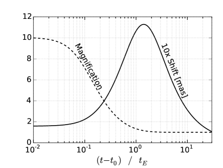
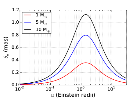
Figure 1.— Left: A characteristic example of the photometric magnification (dashed line) and astrometric shift (solid line) of the lensed source as a function of time since closest approach, normalized to Einstein units. Source magnification is greatest at minimum separation, while the astrometric shift reaches a maximum at $\left(t-t_{0}\right)/t_{E}=\sqrt{2}$. The curves are calculated assuming a 10 M_⊙ lens at a distance of 4 kpc from Earth, a source distance of 8 kpc from Earth, and impact parameter $u_{0}$=0.1. Right: The astrometric shift in the position of a lensed source as a function of the projected separation between the star and the lens, $u$, in units of Einstein radii. The curves are calculated assuming a distance of 8 kpc between the Earth and the star, and a distance of 4 kpc between the Earth and the lens. The three different curves are for lens masses of 1 M_⊙, 5 M_⊙, and 10 M_⊙. The horizontal axis can be converted to units of time using the Einstein-radius crossing time. For the 10 M_⊙ case, the Einstein radius is $\sim$ 4 mas and the crossing time is typically $>$100 days.

In principle, if the Einstein ring is resolvable by interferometric means, $\theta_{E}$ can be measured (Delplancke et al. 2001), but this has yet to be done. For a certain subset of microlensing events, $\theta_{E}$ can be measured from photometry alone using finite source effects, which occur when the source approaches or crosses over a caustic. If the lens is a single object, finite source effects are rarely measurable, requiring a nearly direct passage of the source over the lens (Witt & Mao 1994; Gould 1994b). Even in these fortuitous cases, constraint of $\theta_{E}$ is limited to the precision to which both the microlens parallax and the angular diameter of the source can be measured from photometry and/or spectroscopy (e.g Alcock et al. 1997; Albrow et al. 2000; Yoo et al. 2004; Gould et al. 2009; Zub et al. 2011; Choi et al. 2012), and the most precise mass constraint reported in the literature is $\sim$15%-20% (e.g. Yee et al. 2009). For binary lenses, $\theta_{E}$ is more routinely measured through crossings or close approaches of caustics or cusps. Alternatively, if the lens is luminous and can be viewed at large enough separation from the source after the event, $\boldsymbol{\mu}_{\boldsymbol{\mathrm{rel}}}$ can be measured and $\theta_{E}$ can be determined from Equation 3. In practice, this technique has rarely been used as it requires high resolution imaging, high lens-source relative proper motions (e.g. Alcock et al. 2001; An et al. 2002; Kozłowski et al. 2007; Batista et al. 2015) and is not applicable to faint or non-luminous lenses (i.e. BHs).

Previously, a number of BH candidates have been proposed based on the combination of microlensing parallax measurements with Galactic models that place statistical constraints on $\mu_{\mathrm{rel}}$, and thus on $\theta_{E}$ via Equation 3 (Alcock et al. 1995; Mao et al. 2002; Bennett et al. 2002; Poindexter et al. 2005; Dong et al. 2007; Shvartzvald et al. 2015; Wyrzykowski et al. 2015; Yee et al. 2015). Microlensing parallax measurements are subject to a fourfold degeneracy that arises because the light curve does not distinguish the side on which the lens passes the source (i.e. $\pm u_{0}$ Smith et al. 2003) and the jerk-parallax degeneracy (Gould 2004).

Although the interpretation of microlensing parallax measurements with Galactic models can help to infer ensemble properties of lenses (e.g. cumulative mass and distance distributions), it yields only weak constraints on the lens mass for any single event. It is especially problematic for BH lenses, which might have different spatial and dynamical distributions than stars due to factors such as supernova birth kicks. Alternative approaches are needed to make the first robust detection of an isolated BH.

Astrometric measurements of the lensed source provide a direct measure of $\theta_{E}$ and $\boldsymbol{\mu}_{\boldsymbol{\mathrm{rel}}}$ and thus can be used to overcome the microlensing parallax degeneracies and dependences on Galactic models that have plagued photometric attempts to constrain lens masses. The potential of this technique has been known and studied for over a decade (e.g. Miyamoto & Yoshii 1995; Hog et al. 1995; Walker 1995; Paczyński & Stanek 1998; Boden et al. 1998; Han & Jeong 1999; Jeong et al. 1999; Gould & Yee 2014). During a microlensing event, the images are unresolved, but the center of light is shifted relative to the true position of the source by

$$\boldsymbol{\delta}_{\boldsymbol{c}}(t)=\frac{\theta_{E}}{u(t)^{2}+2}\boldsymbol{u}(t),$$ (8)

(Walker 1995). Combining Equations 4 and 8 yields

$$\boldsymbol{\delta}_{\boldsymbol{c}}(t)=\frac{\theta_{E}}{\tau^{2}+u_{0}^{2}+2}\left[\boldsymbol{u}_{\boldsymbol{0}}+\tau\boldsymbol{\hat{\theta}}_{\boldsymbol{E}}\right].$$ (9)

Figure 1 shows an example of both the photometric and astrometric signal induced as a function of the projected source-lens separation, $u$. Note that the photometric peak occurs at minimum separation, $u=u_{0}$ (at t = $t_{0}$), whereas the maximum astrometric shift occurs at $u=\sqrt{2}$. Typical astrometric shifts, even those induced by $\sim$5 $M_{\odot}$ black holes, are sub-milliarcsecond (mas) in scale (Figure 1). Detections require the high astrometric precision of facilities like the Keck adaptive optics system feeding the NIRC2 instrument. Previous NIRC2 studies have demonstrated astrometric precisions as low as $\sim 0.15$ mas (Lu et al. 2010). Here we use Keck/NIRC2 to make the first ground-based attempt to detect isolated BHs.

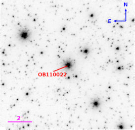
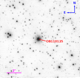
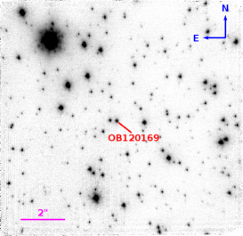
Figure 2.— The three observed 10″x 10″fields centered on the targets of interest: OB110022 (left panel), OB110125 (middle panel), and OB120169 (right panel).

3. Observations

3.1. Photometry from the OGLE survey

We use photometry from the Optical Gravitational Lensing Experiment survey (OGLE, Szymański et al. 2000). OGLE is a continuous, long term survey carried out with the 1.3-m Warsaw telescope at the Las Campanas Observatory in Chile. The survey is currently in its fourth phase (OGLE-IV), with the telescope equipped with a 32-CCD mosaic camera, and focuses on monitoring stars toward the Galactic bulge for microlensing. See Udalski et al. (2015a) for more details on the project. Currently, the OGLE survey discovers, in real time, over 2000 microlensing events per year with its Early Warning System (Udalski 2003). The $I$-band light curves used in this study come from an independent off-line reduction, optimized for these events and using an improved lens position, which used the OGLE photometric pipeline and Difference Image Analysis (DIA) package (Wozniak 2000).

Prior to the 2011 and 2012 astrometric observing seasons, we identified the longest duration events with reasonable magnification ($A_{\rm max}\gtrsim 10$) using the OGLE real-time Early-Warning System (Udalski 2003). In addition, we required that the sources showed no hints of blending and had baseline magnitudes $I\lesssim 19$. We ultimately selected the following three events with long timescales ($t_{\rm E}>130{\rm\,days}$) for astrometric follow-up described in §3.2: OGLE-2011-BLG-0022, OGLE-2011-BLG-0125, and OGLE-2012-BLG-0169 (hereafter OB110022, OB110125, and OB120169). Since the astrometric monitoring had to start near their peaks, the selections could not be done using the full light curves but were instead performed based on modeling the rising part of the light curves prior to their peaks. For two events, OB110022 and OB110125, the light curves ultimately showed significant asymmetry with respect to the peak. The single-lens modeling prior to peak over-estimated the event time scale for both events and binary-lens models are favored. Modeling of the complete photometric dataset is presented in §5.1.

Table 1AO Observations

Event	RA (J2000)	Dec (J2000)	Date	$N_{\mathrm{exp}}$	$N_{\star}$	Strehl	FWHM	$\sigma_{\mathrm{pos}}$	$\sigma_{\mathrm{aln}}$
	[hr]	[deg]	[UT]				[mas]	[mas]	[mas]
OB110022	17:53:17.93	-30:02:29.3	May 25, 2011	27	285	0.14	91	0.56	0.24
			July 7, 2011	16	178	0.13	69	0.66	0.34
			June 23, 2012	40	701	0.24	70	0.31	0.21
			July 10, 2012	34	717	0.26	68	0.25	0.18
			April 30, 2013	22	485	0.24	71	0.30	0.00
			July 15, 2013	30	636	0.34	60	0.20	0.21
OB110125	18:03:32.95	-29:49:43.0	May 23, 2012	21	104	0.10	96	0.39	0.63
			June 23, 2012	33	327	0.36	57	0.09	0.21
			July 10, 2012	18	221	0.21	70	0.25	0.23
			April 30, 2013	48	332	0.29	64	0.13	0.00
			July 15, 2013	39	329	0.36	57	0.12	0.14
OB120169	17:49:51.38	-35:22:28.0	May 23, 2012	5	35	0.10	110	0.84	1.19
			June 23, 2012	10	122	0.24	69	0.38	0.27
			July 10, 2012	22	192	0.29	64	0.22	0.30
			April 30, 2013	31	207	0.29	61	0.17	0.00
			July 15, 2013	11	84	0.26	74	0.47	0.38

3.2. Astrometry with Keck/NIRC2

Astrometric measurements in this study derive from multi-epoch imaging observations of three 10″x 10″fields towards the Galactic Bulge from the W. M. Keck II 10 m telescope. Images were obtained with the near infrared camera, NIRC2 (PI: K. Matthews) behind the laser guide star adaptive optics facility (Wizinowich et al. 2006; van Dam et al. 2006). Figure 2 shows each of the three observed fields, which are centered on OB110022, OB110125, and OB120169 respectively.

Table 1 provides a summary of astrometric observations. Each target was observed in 5–6 epochs spanning 1–2 years. All epochs correspond to the post-peak phase of the microlensing event during which the magnification declines; but the astrometric shift reaches a maximum at $t=t_{0}+t_{E}\sqrt{2-u_{0}^{2}}$ for a single-lens event (see Figure 1).

To aid reconstruction of bad pixels in NIRC2 and avoid detector persistence from bright sources, the telescope was dithered in a continuous random dither pattern with three images taken at each position, with individual integration times of 30 s per frame, split into 10 co-adds $\times$ 3 s in the Kp filter ($1.95-2.30\mu$m) to avoid saturation of the brightest sources. The dither pattern was confined to a small 0$\farcs$7 $\times$ 0$\farcs$7 box to minimize astrometric errors due to residual distortions. The AO/NIRC2 distortion solution is accurate to the $\sim$ 1 mas level (Yelda et al. 2010). For details on this correction we refer the reader to Yelda et al. (2010). The same study derives a plate scale of 9.952 $\pm$ 0.002 mas/pix, which we adopt for our analysis. The visual seeing during May 2011, July 2011, and May 2012 observations was $\sim 2\arcsec$, much worse than average for Mauna Kea conditions, yielding larger astrometric uncertainties in these epochs.

4. Astrometric Data Analysis

4.1. Raw reduction & generation of stellar catalog

Initial reduction of raw data from each epoch of observation was carried out with our custom NIRC2 reduction pipeline (Stolte et al. 2008; Lu et al. 2009) and included flat field and dark calibration, sky subtraction and cosmic ray removal. Corrections for distortion, achromatic differential atmospheric refraction (DAR), and image shifts were applied using the IRAF routine, Drizzle (Fruchter & Hook 2002), as described in Yelda et al. (2010). We note that chromatic DAR effects are small given that all are targets were observed at approximately the same zenith angle in every epoch (Gubler & Tytler 1998). The individual cleaned exposures were co-added, weighted by strehl, to produce a combined image. This summation was restricted to individual frames displaying core FWHM $<1.25~{}\mathrm{FWHM_{min}}$, where $\mathrm{FWHM_{min}}$ is the minimum FWHM of all frames of the particular field and epoch. May 2012 observations of OB110022 were discarded because of poor data quality.

On each combined map, we used the point-spread function (PSF) fitting routine, Starfinder (Diolaiti et al. 2000) to extract a stellar catalog of spatial coordinates and relative brightness. First, the PSFs of a subset of stars (hereafter “PSF stars”) were averaged to derive a mean PSF. The PSF is then cross-correlated with the image and stars were identified as peaks with a correlation above 0.8. To achieve precise centroiding, we locally fit the mean PSF to each identified star. The single-epoch astrometric precision is thus very sensitive to the derivation of the mean PSF and so strict criteria were applied in the selection of PSF stars. Specifically, stars contributed to the mean PSF derivation if they were bright (typically Kp $<$ 18 mag), isolated, and within 4″of the center of the field. The latter criterion avoids detector edge effects and ensures all PSF stars are close to the target of interest, mitigating astrometric error attributed to spatial variation of the PSF caused by instrumental aberrations and atmospheric anisoplanatism. For OB110022 observations in May and July 2011, the PSF showed significant variation across the field and thus a stricter radial cut of $2.5\arcsec$ from the target was applied.

The resulting starlists produced by Starfinder contain positions and fluxes for each star in detector units of pixels and counts, respectively. Fluxes are calibrated using 2MASS K-band magnitudes (Skrutskie et al. 2006) of several bright stars within the field of view and the average brightness for each target is reported in Table 1.

We derive centroiding errors, $\sigma_{pos}$, for each star in each epoch. The centroiding error adopted for each star was the standard error on the mean of its position in three “sub maps”. Each of these sub maps was produced by shifting and co-adding a different third of the frames selected from a Strehl-ranked list such that all sub maps had similar Strehl. A linear translation was then applied to each map, minimizing the astrometric scatter between each sub map and the combined map. The transformation was derived using stars brighter than a cutoff magnitude, $K_{\mathrm{cut}}$. The relative effectiveness of using different $K_{\mathrm{cut}}$ values results from a tradeoff between number of stars and their average brightness. Three values, $K_{\mathrm{cut}}=$ 18, 19 and 20 mag, were tested for each field producing only minor differences in centroiding error. The best precision was achieved using $K_{\mathrm{cut}}$ = 18 mag for the OB110022 field, and 20 for the OB110125, and OB120169 fields. Figures 3-5 show the resulting positional errors, $\sigma_{pos}$ for all stars in each epoch of observation as a function of brightness. In most epochs, the target astrometric precision of 0.15 mas (red line) is achieved for K $\lesssim$ 18 mag.

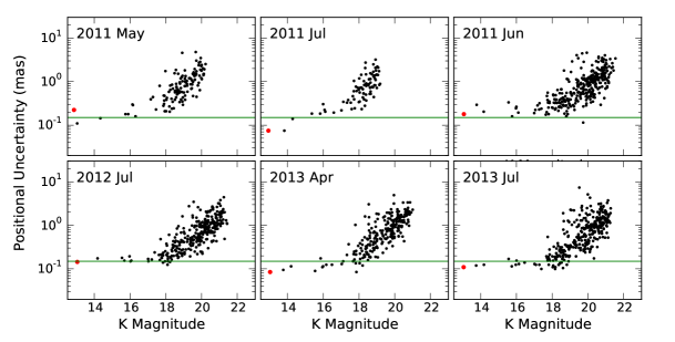
Figure 3.— The centroiding error versus K-band brightness for stars (black points) within 4$\arcsec$ of target OB110022 (red point). Each epoch is presented in a different panel. Centroiding errors are the standard deviation of the star’s mean position in 3 submaps, each composed of the co-addition of a different third of the images. The green lines indicate the desired astrometric precision of 0.15 mas, which is achieved in half of the epochs for K $\lesssim$ 18 mag.

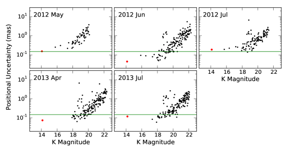
Figure 4.— The centroiding error versus K-band brightness for stars (black points) within 4$\arcsec$ of target OB110125 (red point). Each epoch is presented in a different panel. Centroiding errors are the standard deviation of the star’s mean position in 3 submaps, each composed of the co-addition of a different third of the images. The green lines indicates the desired astrometric precision of 0.15 mas, which is achieved in most epochs for K $\lesssim$ 18 mag.

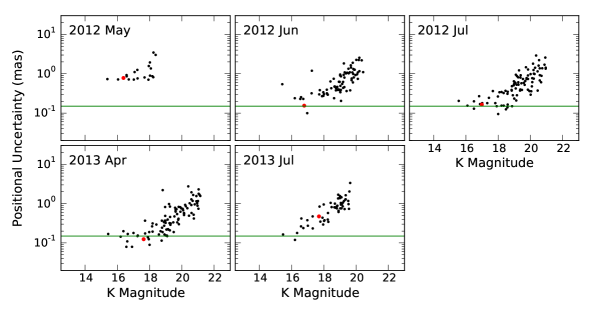
Figure 5.— The centroiding error versus K-band brightness for stars (black points) within 4$\arcsec$ of target OB120169 (red point). Each epoch is presented in a different panel. Centroiding errors are the standard deviation of the star’s mean position in 3 submaps, each composed of the co-addition of a different third of the images. The green lines indicates the desired astrometric precision of 0.15 mas, which is achieved in most epochs for K $\lesssim$ 17 mag.

4.2. Cross-epoch Alignment & Proper Motion Fitting

The first step in computing proper motions is to align images from all epochs into a common coordinate system. Alignment is often complicated by epoch-dependent systematic effects, which can ultimately dominate the proper motion uncertainties. More specifically, changes in instrument conditions and performance (e.g. PSF, pixel scale) from epoch to epoch cause significant variations in relative astrometry. We correct for these systematic effects by transforming combined images from all epochs into the pixel coordinate system of the April 2013 observations using $\chi^{2}$-minimization to find the best-fit linear transformation of spatial coordinates (x, y):

$$x^{\prime}=a_{0}+a_{1}x+a_{2}y+a_{3}x^{2}+...$$ (10)

$$y^{\prime}=b_{0}+b_{1}y+b_{2}x+b_{3}y^{2}+...$$ (11)

where $a_{i}$ and $b_{i}$ are fitted coefficients. This first three terms give a linear transformation independent in $x$ and $y$, effectively correcting for differences in rotation, shear, pixel scale, and translation between star lists from different epochs based on the change in the positions of individual stars. Higher-order transformations are tested and used, when necessary, as discussed further below. The transformation is first performed assuming all stars have zero motion. Proper motions are then derived for the stars and the transformation process is repeated now accounting for the motion of each star. This iterative procedure of deriving the coordinate transformations and stellar proper motions ultimately produces precise relative proper motions in a reference frame that is at rest with respect to the mean motion of all stars within the field.

Note that we have implicitly assumed that the reference stars have negligible parallax. This assumption is supported given that simulated stellar populations using the TRILEGAL galaxy model (Girardi et al. 2012) in the direction of the targets shows that our sample of reference stars is likely composed of $>$83% bulge stars and $>$95% of stars with distances exceeding 5 kpc. Also, the handful of reference stars that can be matched with OGLE sources at I-band, given the limited OGLE spatial resolution, have I$-$Kp colors consistent with highly extincted, thus distant, bulge stars.

The quality of the cross-epoch alignment depends on several factors, including which stars are used to find the best-fit transformation, how these stars are weighted, and the order of the transformation equations. The sample of stars used to derive the transformation was restricted to those detected in all epochs and within 4″of the microlensing targets. The microlensing targets were omitted since their motion would not be linear if they are lensed. We further restricted the astrometric reference stars to bright stars and we tested brightness cuts of $K_{\mathrm{cut}}=$ 18, 20, and 22 mag. Extending the reference star sample from $K_{\mathrm{cut}}=$ 18$\rightarrow$20 significantly improves the cross-epoch alignment since the number of reference stars increases from 0-100 to $>$400. Some epochs are sufficiently deep that extending from $K_{\mathrm{cut}}=$ 20$\rightarrow$22 added $>$100 more stars to the sample. Therefore, we adopted $K_{\mathrm{cut}}=$ 22 for all of the targets and epochs. The astrometric reference stars were weighted based on positional uncertainties, as outlined in Appendix A; and we find that the proper motion fits are independent of our choice of weighting scheme. We also tested different orders (O=1,2,3) of polynomial transformations between each epoch using an F-test (Appendix B). OB110022 shows minimal improvement when advancing to 2nd order, therefore we adopt O$=$1 for this source. OB110125 and OB120169 showed improvement going from O$=1\rightarrow 2$, therefore we adopted O$=$2 for these sources. We note that microlensing fits were ultimately run for both O$=$1 and O$=$2 for both OB110022 and OB120169 and there was negligable change in the final lens-mass posteriors.

In addition to the random error on the position of each star, $\sigma_{pos}$, there is additional error due to uncertainties in the coordinate frame alignment. To capture this alignment error, a half-sample bootstrap resampling analysis is performed to derive the transformation parameters using different half-sample sets of stars (Babu & Feigelson 1996). The alignment error, $\sigma_{aln}$, for each star is taken as the standard deviation of the transformed positions from all the samples (see Ghez et al. 2000, 2005; Clarkson et al. 2012, for further justification). The alignment error is typically smaller than the average centroiding error for all stars and is independent of brightness. However, the alignment errors produce comparable uncertainties for the O=2 transformations that we have adopted for OB110125 and OB120169, likely due to the small number of bright stars that dominate the alignment and systematic errors from PSF variations over the field of view. Table 1 presents the median positional and alignment error for each epoch for all stars with r$<$4” and Kp$<$19 mag. The final positional error adopted for each lensing target is $\sigma=\sqrt{\sigma_{pos}^{2}+\sigma_{aln}^{2}}$ and is, on average, $\sim$0.26 mas for OB110022, $\sim$0.34 mas for OB110125, and $\sim$0.68 mas for OB120169 for each epoch.

Proper motions are fit for all stars in the field of view. To evaluate the quality of the final cross-epoch transformations, we examine the distribution of $\chi^{2}_{vel}$ values from the proper motion fits for all of the unlensed stars detected in all epochs (Figure 6). These $\chi^{2}_{vel}$ values are calculated from the residuals from the proper motion fits for each star, weighted by the total uncertainty, $\sigma$, which includes both positional and alignment errors. The distribution of $\chi^{2}_{vel}$ for all the stars is expected to follow a standard $\chi^{2}$ distribution with $2*(N_{\mathrm{epochs}}-2)$ degrees of freedom (2 free parameters in the velocity fit in each direction), which is also shown in Figure 6. Deviations from the expected distribution are likely due to systematic errors (e.g. spatial PSF variations) that cannot be captured with simple error re-scaling techniques. Reducing or accounting for these systematic errors is the subject of on-going adaptive optics PSF modeling projects (e.g. Britton 2006; Fitzgerald et al. 2012) and is beyond the scope of this paper.

For each lensing target, the final positions and uncertainties at each epoch used for both the proper motion and microlens fits are presented in Tables 2, 3, and 4. All positions are reported as relative offsets to the mean position with positive values increasing to the East and the North.

Table 2OB110022 Measurements

MJD	Kp	$\Delta x_{E}$	$\Delta x_{N}$	$\sigma_{\mathrm{E}}$		$\sigma_{\mathrm{N}}$
		[mas]	[mas]	[mas]		[mas]
				pos	aln	pos	aln
55706.540	12.9	-5.06	-2.96	0.29	0.19	0.16	0.13
55749.273	12.9	-3.84	-2.55	0.09	0.26	0.06	0.23
56101.366	13.1	0.26	-0.46	0.22	0.11	0.14	0.14
56118.168	13.0	0.35	0.06	0.12	0.08	0.17	0.15
56412.553	13.0	3.64	2.92	0.04	0.00	0.13	0.00
56488.158	13.0	4.65	2.99	0.11	0.09	0.11	0.14

Table 3OB110125 Measurements

MJD	Kp	$\Delta x_{E}$	$\Delta x_{N}$	$\sigma_{\mathrm{E}}$		$\sigma_{\mathrm{N}}$
		[mas]	[mas]	[mas]		[mas]
				pos	aln	pos	aln
56070.686	14.1	-0.17	0.88	0.18	0.48	0.13	0.54
56101.366	14.1	0.46	-0.09	0.05	0.24	0.04	0.18
56118.533	14.1	0.49	-0.02	0.22	0.20	0.16	0.28
56412.553	14.1	-0.41	-0.55	0.07	0.00	0.08	0.00
56488.523	14.2	-0.36	-0.21	0.09	0.13	0.15	0.15

Table 4OB120169 Measurements

MJD	Kp	$\Delta x_{E}$	$\Delta x_{N}$	$\sigma_{\mathrm{E}}$		$\sigma_{\mathrm{N}}$
		[mas]	[mas]	[mas]		[mas]
				pos	aln	pos	aln
56070.686	16.4	1.01	-0.92	1.08	0.72	0.48	1.00
56101.366	16.8	0.20	-0.32	0.11	0.26	0.20	0.24
56118.533	17.0	0.32	-0.30	0.18	0.32	0.15	0.25
56412.553	17.6	-0.73	0.46	0.16	0.00	0.09	0.00
56488.523	17.7	-0.81	1.07	0.07	0.25	0.88	0.34

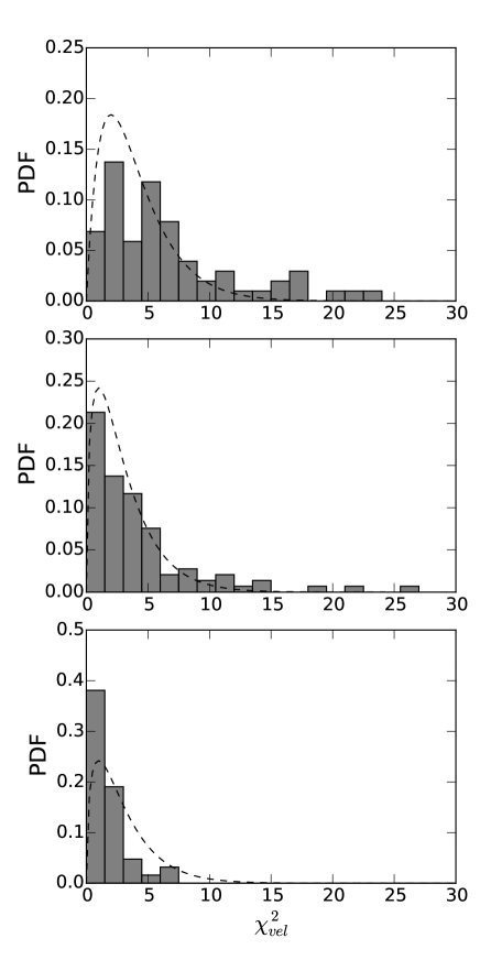
Figure 6.— Distribution of $\chi^{2}_{\mathrm{vel}}$ for all stars around OB110022 (left), OB110125 (center), and OB120169 (right).

5. Fitting Microlensing Models

5.1. Photometry-only

Microlensing models are fit to the OGLE $I$-band light curves of the three lensed sources using a Markov Chain Monte Carlo (MCMC) analysis. A standard point-source-point-lens (PSPL) model is first fit to each event, taking into account microlens parallax effects (Gould 2004). The PSPL model includes seven free parameters, including $t_{0}$, $u_{0}$, $t_{E}$, and the East and North components of the microlensing parallax vector, $\pi_{E,N}$ and $\pi_{E,E}$. The final two parameters are the baseline (i.e. unlensed) flux of the source, $f_{s}$, and the flux from blended sources, $f_{b}$, that might be in the photometric aperture. We consider the twofold degeneracy ($u_{0}>0$ / $u_{0}<0$) (Gould 2004), which we denote as $u_{0}^{+}$ and $u_{0}^{-}$ solutions respectively.

A PSPL model with parallax adequately describes the OB120169 light curve. In contrast, fits to the light curves of OB110022 and OB110125 are poor. These latter light curves have much steeper slopes during the post-maximum phases compared to the pre-maximum phases. We find that in both cases, binary-lens models with microlens parallax provide substantially better fits to the light curves.

For the binary-lens model, we introduce three additional parameters, mass ratio $q$, projected binary separation $s$ in the units of the Einstein radius, and position angle $\alpha$ between the source trajectory and the binary axis. Note that this assumes that the binary lens orbital motion is negligible. In a similar fashion to Dong et al. (2007), we search for the best-fit solutions via an MCMC and consider the four-fold degeneracy (close/wide binary (Dominik 1999) and $u_{0}^{+}/u_{0}^{-}$).

This 10-parameter binary lens model provides a satisfactory fit to the OB110125 data. However, the fit to the OB110022 light curve showed significant residual structure. We considered that these second-order effects might arise from orbital motion of the binary lens. To test this hypothesis, we introduced two additional model parameters, time derivatives of projected binary separation $\dot{s}/s$ and rotation angle $\Omega$. The non-static solution is a significant improvement over the static solution.

Given the similarity in their deviations from the PSPL models (slow rise and steep fall), we consider the possibility that OB110022 and OB110125 are not genuine microlensing events; but, instead, belong to a previously unknown class of long-period variable stars. One unique characteristic of microlensing events is that the magnification is achromatic (unless there are significant finite-source effects, of which there is no evidence in the light curves in this study). For variable stars, the changes in flux are generally associated with variations in color. We use the sparsely-covered OGLE $V$-band data during the events (with a cadence of roughly once per 10 days) to check the color variations. With model-independent linear-regression, the colors do not change at the level of photometric precision ($1\%$) during the event, consistent with the microlensing interpretation.

5.2. Astrometric model with photometric priors

We fit an astrometric lensing model to our NIRC2 data in order to measure lens masses. We adopt simple point-source, point-lens astrometry models for all three cases. In principle, a binary-lens model should be adopted for OB110022 and OB110125. However, in the limit where the observations are consistent with linear proper motion and no astrometric lensing signal is detected, which is the case for all three of our targets (see §6.1), the PSPL should be sufficient for estimating mass constraints. We also ignore parallax effects when modeling the astrometry. As shown by Boden et al. (1998) and Han & Chang (2000), microlens parallax has negligible effect on the astrometric microlensing signals given our astrometric precision. For the final best-fit PSPL astrometric models, we confirm that parallax effects shift the expected astrometric positions typically by less than 0.10 mas and always less than 0.2 mas, within our measurement uncertainty.

We employ a Bayesian inference method to model the astrometry. Posterior probability distributions derived from the photometric MCMC analysis (§5.1) are used as priors in our astrometric fits. Although this model ignores the parallactic perturbation of the astrometric signal, it still makes use of the photometrically measured $\pi_{E}$. The free parameters are: $t_{0}$, $t_{E}$, $u_{0}$, $\pi_{E}$, $\boldsymbol{\mu}_{\boldsymbol{s}}$, $\boldsymbol{\mu}_{\boldsymbol{\mathrm{rel}}}$ and $\boldsymbol{X}_{\boldsymbol{{0}}}$, which is the intrinsic source position on the plane of the sky $\left[x_{E},x_{N}\right]$ at $t=t_{0}$, denoted by East and North components.

The apparent position of the source in the sky plane is modeled as

$$\boldsymbol{X}\left(t\right)=\boldsymbol{X}_{\boldsymbol{{0}}}+\boldsymbol{\mu}_{\boldsymbol{s}}\left[t-t_{0}\right]+\boldsymbol{\delta}_{\boldsymbol{c}}\left(t\right)$$ (12)

where $\boldsymbol{\delta}_{\boldsymbol{c}}\left(t\right)$ is given by Equation 9. Both $\theta_{E}$ and $M$ are implicitly defined by each astrometric model via Equations 3 and 7 respectively.

The probability of different microlensing event models given our astrometry is evaluated in the following Bayesian framework. According to Bayes theorem, the probability, $P$, of any microlensing model $m$($t_{0}$, $t_{E}$, $u_{0}$, $\pi_{E}$, $\boldsymbol{\mu}_{\boldsymbol{s}}$, $\boldsymbol{\mu}_{\boldsymbol{\mathrm{rel}}}$, $\boldsymbol{X}_{\boldsymbol{{0}}}$) given astrometric measurements $d\left(x_{E}^{\mathrm{obs}},x_{N}^{\mathrm{obs}}\mid t^{\mathrm{obs}}\right)$ is

$$P({m\mid d})\propto P({d\mid m})P(m)$$ (13)

where $P(m)$ is the prior probability of $m$ and $P({d\mid m})$ is the likelihood of the observed data given $m$. We adopt:

$$P({d\mid m})=e^{-\chi^{2}/2}$$ (14)

where

$$\chi^{2}=\sum_{i}\left(\left[\frac{x_{E,i}^{\mathrm{obs}}-x_{E,i}^{\mathrm{mod}}}{\sigma_{E,i}}\right]^{2}+\left[\frac{x_{N,i}^{\mathrm{obs}}-x_{N,i}^{\mathrm{mod}}}{\sigma_{N,i}}\right]^{2}\right).$$ (15)

Here, $\left[x_{E,i}^{\mathrm{obs}},x_{N,i}^{\mathrm{obs}}\right]$ are the observed positions at time $t^{obs}_{i}$ in the East and North directions, $\left[\sigma_{E,i},\sigma_{N,i}\right]$ are the corresponding astrometric uncertainties on this observation, and $\left[x_{E,i}^{\mathrm{mod}},x_{N,i}^{\mathrm{mod}}\right]$ are the predicted model positions.

The joint posterior distributions for $u_{0}$, $t_{0}$, $t_{E}$, and $\boldsymbol{\pi}_{E}$ derived from photometric modeling (§5.1) serve as priors for our astrometric microlensing models. We adopt uniform priors on all other model parameters. In particular, the priors on the source and lens proper motions are uniform within the range $[-40,40]$ mas yr^-1. While previous microlensing studies have incorporated priors based on Galactic models, it is unclear whether BHs have similar distance or velocity distributions as luminous stellar populations. The proper motions of the background sources can be well-constrained by several years of astrometric observations without relying on Galactic models.

To compute parameter posterior distributions, we use a publicly available Bayesian inference package, MultiNest (Feroz et al. 2009, 2013), which employs a nested sampling algorithm (Skilling 2006). MultiNest explores parameter space more quickly and effectively than traditional MCMC algorithms when parameters are strongly correlated and parameter space is multimodal. For each sampling iteration, the Bayesian evidence is computed at a fixed number of points N, iteratively converging towards smaller volumes of parameter space with the highest evidence. The routine terminates when the iterative increase in evidence falls below some tolerance, E_tol. We find that N = 1000, E_tol=0.3 produces adequate results.

6. Results

6.1. Proper motion fits: No lensing

The resulting proper motions for the targets and all other stars within 4″  have precisions of $<$0.5 mas yr^-1 (Figure 7). The target with the highest quality data, OB110022, has proper motion precisions of $<$0.2 mas yr^-1 for stars brighter than $K<17$ mag. Given a reasonably stable atmosphere in future experiments, proper motion errors of $<0.1$ mas yr^-1 are obtainable.

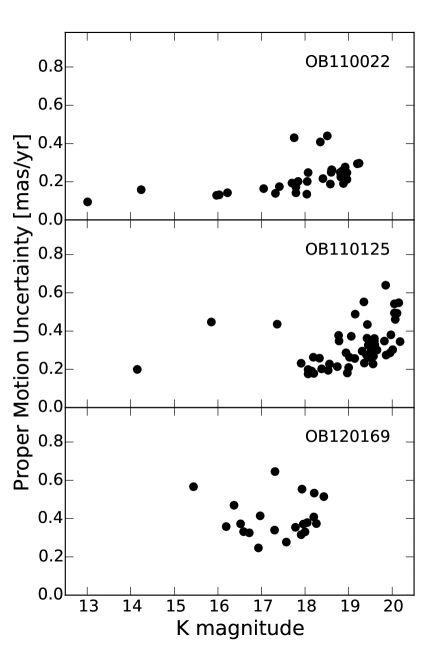
Figure 7.— Errors on the fitted proper motion plotted against source brightness for the OB110022 (top), OB110125 (middle) and OB120169 (bottom) fields. Plotted errors are the average over X and Y.

The best-fit proper motions for the three targets of interest and the associated errors are shown in Table 5. Figures 8-10 show the proper motion fits for the targets and five of the brightest stars closest to each of them, which serve as comparison samples. The corresponding residuals are also shown. There are clearly some residual systematics affecting each target uniquely, but the consistency of the entire ensemble of residuals with the measured Gaussian errors suggests that we cannot do much better given the poor atmospheric conditions under which much of the data was obtained. The relatively comparable frequency of outliers in the comparison sample relative to the target of interest suggests that points deviating far from the proper motion fit cannot be interpreted as a lens induced signature without proper astrometric modeling and comparison with a reference sample.

The three targets of interest are all consistent with linear motion (Figure 11). The $\chi^{2}$ of the target’s proper motion fit is not a significant outlier when compared to all other stars in the field with K$<$22 mag and detected in all epochs. Specifically, OB110022 has a $\chi^{2}=22.2$ (for 8 degrees of freedom (DOF)) and 21% of the comparison sample have higher $\chi^{2}$ values, OB110125 has a $\chi^{2}=27.6$ (for 6 DOF) and 16% of the comparison sample have higher $\chi^{2}$ values, and OB120169 has a $\chi^{2}=1.1$ (for 6 DOF) and 86% of the comparison sample have higher $\chi^{2}$ values. The distributions of $\chi^{2}$ values from the proper motion fits for the complete sample of reference stars in the fields around all three targets are plotted in Figure 25 (Appendix B).

While we do not detect significant astrometric microlensing in any of the three targets, the strong limits on any non-linearity in the case of OB110022 allow us to constrain the properties of the source-lens system as shown in §6.2.3. We note that although the $\chi^{2}$ distribution for OB110022 is skewed to higher values than expected for the adopted O=1 transformation, the larger astrometric error bars produced in fits using O=2 produced a negligable change in the final lens-mass posteriors.

Table 5Proper Motions

Source	$\mu_{E}$	$\mu_{N}$
	[mas yr-1]	[mas yr-1]	$\chi_{vel}^{2}$	DOF
OB110022	4.22 $\pm$ 0.09	2.96 $\pm$ 0.09	22.2	8
OB110125	-0.82 $\pm$ 0.20	-0.53 $\pm$ 0.19	10.4	6
OB120169	-1.11 $\pm$ 0.28	0.96 $\pm$ 0.27	1.1	6

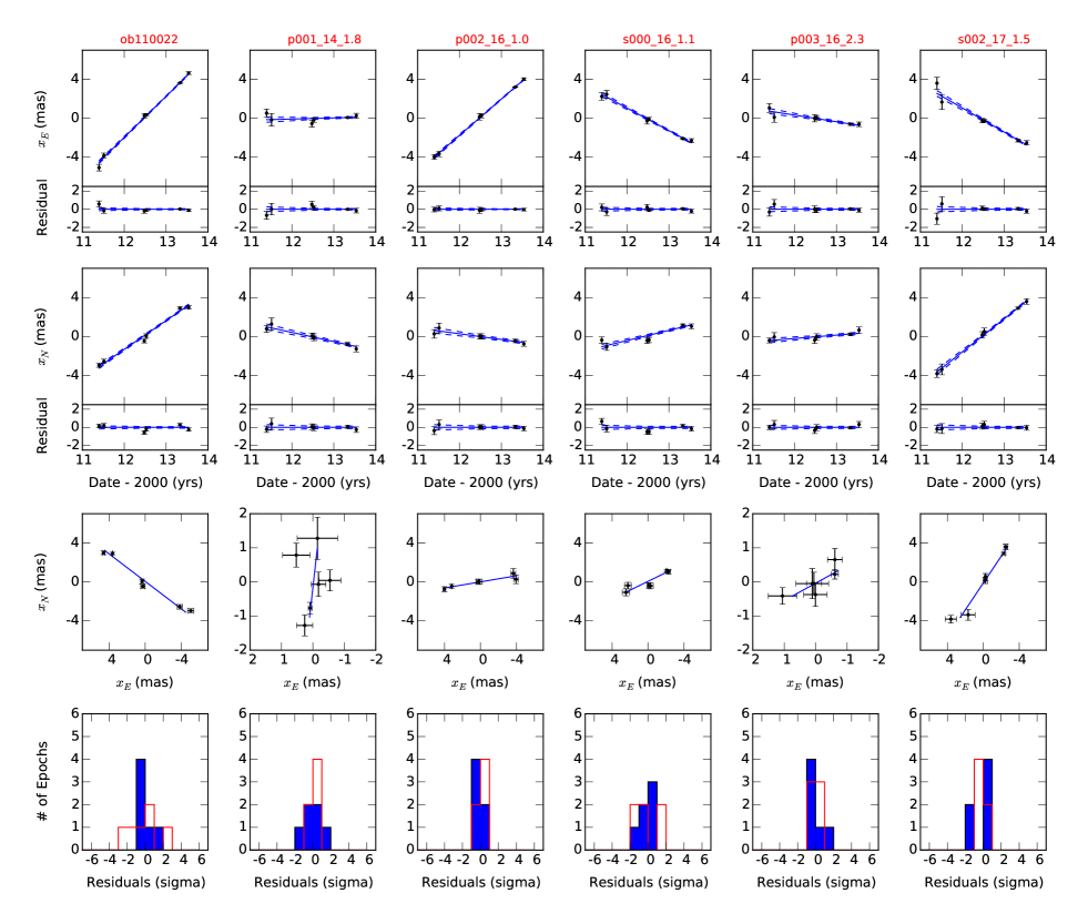
Figure 8.— Proper motion fits to OB110022 (leftmost column) and five comparison sources (one per column), which are both bright and near OB110022. Sources names are given in red. The three numbers in the names of the comparison sources correspond to a catalog number, K magnitude, and arcseconds from OB110022. The rows are explained as follows: (Row 1) Linear proper motion fits to the East component, $x_{E}$, of the astrometric time-series points (black). The dashed blue line correspond to 1-sigma errors on the proper motion fit. Corresponding residuals to the proper motion fit are shown. (Row 2) Same as Row 1 but for North component, $x_{N}$, of astrometry time-series. (Row 3) Linear fits to the proper motion in the sky plane. (Row 4) Histogram of residuals to the proper motion fits in $x_{E}$ (red) and $x_{N}$ (blue) in units of their 1-sigma error bars.

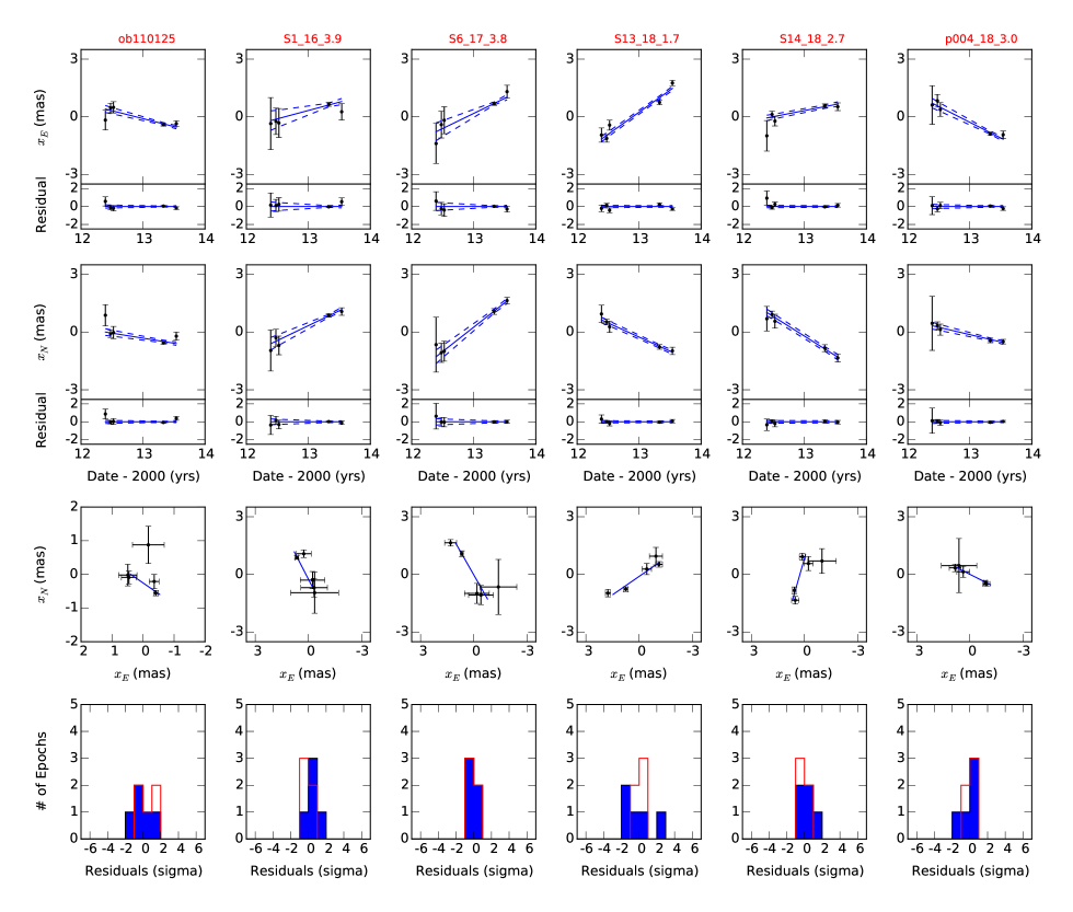
Figure 9.— Same as Figure 8 but for the OB110125 field.

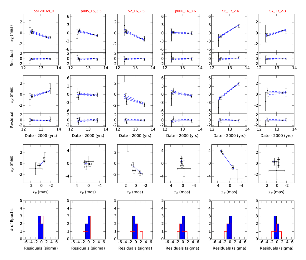
Figure 10.— Same as Figure 8 but for the OB120169 field.

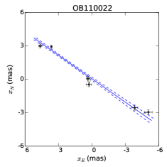
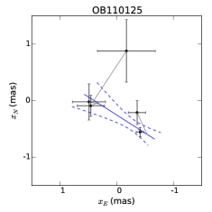
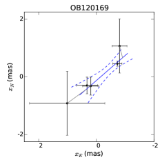
Figure 11.— A zoomed-in view of the proper motion fits for OB110022 (left), OB110125 (middle), and OB120169 (right). Observed positions on the sky plane are shown as black points. The best-fit proper motion and 1$\sigma$ uncertainties are shown in blue.

6.2. Lens Masses

6.2.1 OB120169

Figure 12 shows the OGLE $I$-band light curve as well as the best-fitting photometric microlensing model, which has a single, isolated lens. Table 6 lists the medians and 68% confidence intervals of the posterior distributions for each model parameter derived from photometry and from astrometric models informed by photometric priors. We include both the $u_{0}^{+}$ and $u_{0}^{-}$ solutions because neither is strongly preferred in the fit. While we utilize the Bayesian evidence in our fitting procedure, it is useful to compare the resulting $\chi^{2}$ of the best-fit astrometric lensing solution ($\chi^{2}=1.13$ for 1 DOF) to that of the linear proper motion fit ($\chi^{2}=1.10$ for 6 DOF). In this case, the lensing model did not yield a significant improvement in the $\chi^{2}$ value over the linear proper motion model.

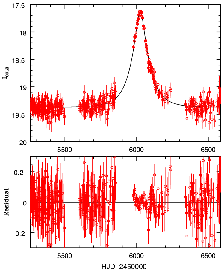
Figure 12.— Top: Light curve of OB120169. Red points indicate OGLE measurements. The black line represents the best-fitting point-source-point-lens model, which includes microlensing parallax. Bottom: Residuals to best-fitting model.

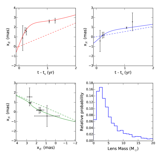
Figure 13.— Left: Top: Fitted astrometric data (black points) for OB120169, with the best-fitting astrometric model over-plotted in $x_{E}$ (red solid line) and $x_{N}$ (blue solid line) versus time after minimum source-lens separation. Dashed lines indicate unlensed source motions. The joint posterior probability distributions for $u_{0}<0$, $t_{0}$, $t_{E}$, $\pi_{E,N}$, and $\pi_{E}$ from light-curve fitting are adopted as priors for astrometric model fitting. A single single point-source-point-lens astrometric model is used that ignores the effects of source-lens relative parallax. Bottom Left: Same as top, but shown in the sky plane. Bottom Right: Lens mass posterior probability distribution.

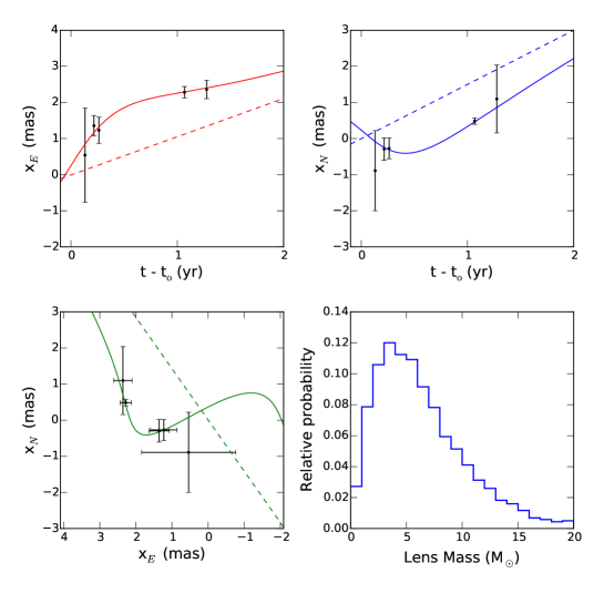
Figure 14.— Same as Figure 13 but adopting the joint posterior probability distributions for $u_{0}>0$, $t_{0}$, $t_{E}$, and $\pi_{E}$ from our light-curve fitting as priors for our astrometric model fitting.

Figures 13 and 14 display the best fitting astrometric microlensing models and lens mass constraints corresponding to the $u_{0}^{+}$ and $u_{0}^{-}$ solutions respectively. The lens mass posterior associated with the $u_{0}^{-}$ solution has a median of 5.7 M_⊙, but wide 1-sigma and 3-sigma confidence intervals of 4.0–7.7 and 0.4–39.8 M_⊙ respectively. The $u_{0}^{+}$ solution has a median of 4.0 M_⊙ and similarly wide 1-sigma and 3-sigma confidence intervals of 2.6–6.2 and 0.2–38.8 M_⊙ respectively. The best-fitting models for $u_{0}^{-}$ and $u_{0}^{+}$ solutions are shown in Figures 13 and 14. Both solutions predict that the y-component of the source apparent motion has started to turnover and approach linear, unlensed motion. Future observations are essential to determine if this turnover continues and will place a more conclusive constraint on the lens mass, possibly verifying a black hole.

Table 6Microlensing Event Parameters - OB120169

	$u_{0}^{-}$ Solution		$u_{0}^{+}$ Solution
Parameter	Photometry	Astrometry	Photometry	Astrometry
$t_{0}$ (HJD - 2450000)	6026.03${}^{+0.43}_{-0.40}$	6026.04${}^{+0.28}_{-0.28}$	6026.25${}^{+0.43}_{-0.38}$	6026.27${}^{+0.29}_{-0.26}$
$u_{0}$	-0.222${}^{+0.033}_{-0.031}$	-0.229${}^{+0.024}_{-0.025}$	0.166${}^{+0.044}_{-0.070}$	0.165${}^{+0.026}_{-0.042}$
$t_{E}$ (days)	135${}^{+21}_{-36}$	121${}^{+9}_{-15}$	156${}^{+32}_{-42}$	157${}^{+23}_{-21}$
$\pi_{E,E}$	-0.058${}^{+0.017}_{-0.018}$	-0.057${}^{+0.014}_{-0.014}$	-0.031${}^{+0.018}_{-0.016}$	-0.030${}^{+0.012}_{-0.011}$
$\pi_{E,N}$	0.11${}^{+0.30}_{-0.12}$	-0.11${}^{+0.19}_{-0.23}$	0.14${}^{+0.11}_{-0.05}$	0.14${}^{+0.06}_{-0.04}$
$\mu_{s,E}~{}(\mathrm{mas~{}yr^{-1})}$	—	-1.15${}^{+0.48}_{-0.53}$	—	-0.96${}^{+0.53}_{-0.51}$
$\mu_{s,N}~{}(\mathrm{mas~{}yr^{-1})}$	—	0.85${}^{+0.51}_{-0.52}$	—	1.05${}^{+0.64}_{-0.63}$
$\mu_{\mathrm{rel},E}~{}(\mathrm{mas~{}yr^{-1})}$	—	-3.8${}^{+14.7}_{-14.5}$	—	-4.2${}^{+10.8}_{-11.5}$
$\mu_{\mathrm{rel},N}~{}(\mathrm{mas~{}yr^{-1})}$	—	1.2${}^{+14.9}_{-15.0}$	—	1.5${}^{+13.4}_{-13.8}$
$\theta_{E}$ (mas)	—	5.9${}^{+3.0}_{-3.9}$	—	6.3${}^{+3.3}_{-4.4}$
Mass ($M_{\odot}$)	—	4.0${}^{+2.3}_{-6.4}$	—	5.6${}^{+3.1}_{-5.1}$
$I_{\mathrm{OGLE}}$	19.266${}^{+0.181}_{-0.195}$	—	19.641${}^{+0.456}_{-0.386}$	—
$f_{b}/f_{s}$	-0.10${}^{+0.14}_{-0.17}$	—	0.27${}^{+0.43}_{-0.54}$	—
$\chi^{2}$	428.5	1.1	424.7	1.3
Ndof	433	1	433	1

6.2.2 OB110022

Figure 15 shows the OGLE $I$-band light curve as well as the best-fitting photometric microlensing model, which has a non-static, binary lens. Table 7 lists the posterior medians and 68% confidence intervals for each OB110022 event parameter. We separately list measurements derived from photometry only, and from astrometric modeling informed by photometric priors. The blended flux $f_{b}$ is comparable to the source flux $f_{s}$. However, we note that $f_{b}$ increased substantially when adopting the non-static solution, which may indicate that more detailed modeling is required. The median of the posterior for binary separation $s$ = 0.42 suggesting that the binary separation is small compared to the Einstein radius. The light curve is relatively smooth indicating that there are no caustic approaches or crossings that would lead to additional, binary-induced non-linearity in the apparent source trajectory (Sajadian 2014). Additionally, no such non-linearity is detected in the astrometry and the highly linear proper motion measured for OB110022 is therefore consistent with its smooth light curve.

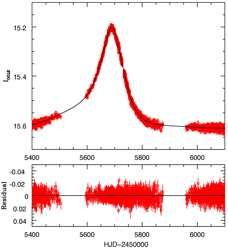
Figure 15.— Top: Light curve of OB110022. Red points indicate OGLE measurements. The black line represents the best-fitting binary lens model, which includes microlensing parallax and binary orbital motion. Bottom: Residuals to best-fitting model.

No significant astrometric lensing signal is detected. The best-fitting lensing model for the astrometry gives a $\chi^{2}=21.2$ (3 DOF), which is not a significant improvement over the linear proper motion model ($\chi^{2}=22.2$ for 8 DOF). Given that the lensing event was well sampled during the period of maximum astrometric shift (Eq. 8), the degree of linearity allows us to put constraints on the lens mass. Figure 16 displays the posterior probability distribution for the OB110022 lens mass and the best-fitting astrometric model. Most notably, the posterior corresponding to the total lens mass $M$ has a median of 0.67 M_⊙ with 1-$\sigma$ and 3-$\sigma$ confidence intervals of 0.51–0.83 M_⊙ and 0.05–1.79 M_⊙, respectively. The highest masses correspond to large relative proper motions between the source and lens ($\mu_{\mathrm{rel}}>20$ mas yr^-1 for M$>$1 M${}_{\odot}~{}$). Combining $M$ and $q$, the individual masses of the binary lens objects are $\sim$0.5 M_⊙ and 0.1 M_⊙, consistent with some combination of K- or M-dwarfs and white dwarfs. This lens is extremely unlikely to contain a black hole. Constraint of the lens objects to such low masses is not surprising given the high degree of linearity of the measured source motion, combined with relatively low astrometric error and multi-year time baseline.

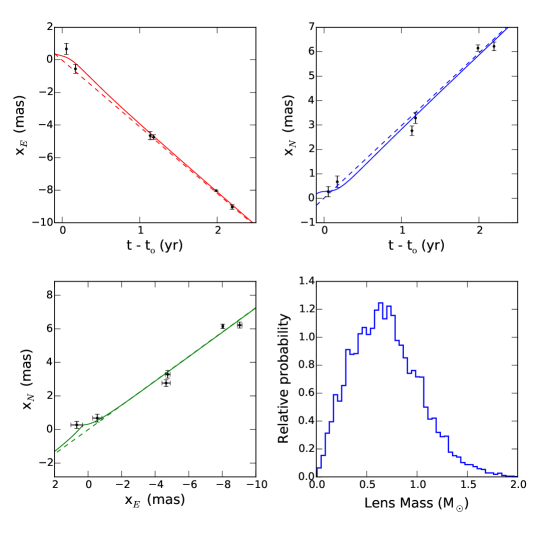
Figure 16.— Top: Fitted astrometric data (black points) for OB110022, with the best-fitting astrometric model over-plotted in $x_{E}$ (red solid line) and $x_{N}$ (blue solid line) versus time after minimum source-lens separation. Dashed lines indicate unlensed source motions. The joint posterior probability distributions for $u_{0}$, $t_{0}$, $t_{E}$, $\pi_{E,N}$, and $\pi_{E}$ from light-curve fitting are adopted as priors for astrometric model fitting. A single single point-source-point-lens astrometric model is used that ignores the effects of source-lens relative parallax. Bottom Left: Same as top, but shown in the sky plane. Bottom Right: Lens mass posterior probability distribution.

Table 7Microlensing Event Parameters - OB110022

Parameter	Photometry	Astrometry
$t_{0}$ (HJD - 2450000)	5687.91${}^{+0.26}_{-0.27}$	5687.41${}^{+0.25}_{-0.26}$
$u_{0}$	0.573${}^{+0.019}_{-0.020}$	0.574${}^{+0.018}_{-0.019}$
$t_{E}$ (days)	61.4${}^{+1.0}_{-1.0}$	61.4${}^{+0.9}_{-0.9}$
$\pi_{E,E}$	-0.393${}^{+0.013}_{-0.012}$	-0.393${}^{+0.013}_{-0.012}$
$\pi_{E,N}$	-0.071${}^{+0.013}_{-0.014}$	-0.071${}^{+0.014}_{-0.014}$
$\mu_{s,E}~{}(\mathrm{mas~{}yr^{-1})}$	—	4.06${}^{+0.16}_{-0.16}$
$\mu_{s,N}~{}(\mathrm{mas~{}yr^{-1})}$	—	3.02${}^{+0.20}_{-0.20}$
$\mu_{\mathrm{rel},E}~{}(\mathrm{mas~{}yr^{-1})}$	—	-7.3${}^{+8.7}_{-8.8}$
$\mu_{\mathrm{rel},N}~{}(\mathrm{mas~{}yr^{-1})}$	—	-5.5${}^{+8.0}_{-7.6}$
$\theta_{E}$ (mas)	—	2.19${}^{+1.06}_{-1.17}$
Mass ($M_{\odot}$)	—	0.67${}^{+0.32}_{-0.37}$
s	0.423${}^{+0.006}_{-0.006}$	—
q	0.191${}^{+0.009}_{-0.010}$	—
$\alpha$	4.794${}^{+0.014}_{-0.015}$	—
$\omega$	0.062${}^{+0.006}_{-0.007}$	—
$\dot{s}/s$	0.468${}^{+0.015}_{-0.020}$	—
$I_{\mathrm{OGLE}}$	16.264${}^{+0.057}_{-0.054}$	—
$f_{b}/f_{s}$	0.82${}^{+0.73}_{-0.91}$	—
$\chi^{2}$	9235	20.8
Ndof	8253	3

6.2.3 OB110125

Figure 17 shows the OGLE $I$-band light curve as well as the best-fitting photometric microlensing model for OB110125, which has a static binary lens. The [wide, $u_{0}^{-}$] solution is preferred and shown in Figure 17. Table 8 lists the posterior medians and 68% confidence intervals for each OB110125 model parameter.

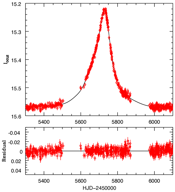
Figure 17.— Top: Light curve of OB110125. Red points indicate OGLE measurements. The black line represents the best-fitting binary lens model, which includes microlensing parallax, but does not include binary orbital motion. Bottom: Residuals to best-fitting model.

Lens mass measurements of OB110125 are omitted because the first astrometric observation took place too long after the event peak. The light curve fitting favors a binary lens model with an Einstein crossing time of $\sim$63 days, and the first observation of OB110125 was $\sim$ 347 days after the event peak (5.5 x $t_{E}$), at which point the non-linear, lens-induced motion evolves too slowly to detect. In principle, the lens mass could still be estimated by a joint analysis of the measured source proper motion, photometrically constrained event parameters ($t_{E}$, $\boldsymbol{\pi}_{E}$), and a Galactic model (Yee et al. 2015, e.g.). However, we choose to avoid relying on models of the spatial and kinematic distributions of Galactic objects, especially those of BHs, which carry large uncertainties.

Table 8Microlensing Event Parameters - OB110125

Parameter	Photometry
$t_{0}$ (HJD - 2450000)	5724.43${}^{+0.72}_{-0.70}$
$u_{0}$	-0.611${}^{+0.031}_{-0.030}$
$t_{E}$ (days)	62.9${}^{+2.4}_{-2.6}$
$\pi_{E,E}$	0.515${}^{+0.034}_{-0.033}$
$\pi_{E,N}$	-0.437${}^{+0.036}_{-0.037}$
s	3.11${}^{+0.11}_{-0.11}$
q	1.07${}^{+0.16}_{-0.17}$
$\alpha$	3.517${}^{+0.008}_{-0.009}$
$I_{\mathrm{OGLE}}$	15.54${}^{+0.16}_{-0.17}$
$f_{b}/f_{s}$	-0.035${}^{+0.129}_{-0.160}$
$\chi^{2}$	1012.7
Ndof	995

7. Discussion

Despite the unusually poor seeing conditions in which most of our data were collected, and a time-sampling of lensing events that was far less than optimal, we have demonstrated the feasibility of detecting black holes via astrometric methods, given better observing conditions and a well-timed set of observations over a longer (several year) baseline. While we have not yet detected a significant astrometric microlensing signal, we achieved astrometric precisions in a few epochs, when seeing was not poor, that would be sufficient to trace the lens-induced astrometric shifts due to a black hole lens.

A binary lens model is favored for two of the three events, OB110022 and OB110125. We measure the OB110022 combined lens mass to better than $\sim$50%. This mass constraint is likely comparable to those achieved by using finite source effects to estimate the source angular size, $\theta_{\star}$ (e.g. Park et al. 2013, 2015; Jung et al. 2015; Zhu et al. 2015). One event, OB120169, is consistent with an isolated lens, which remains a BH candidate. The best-fitting astrometric models for both $u_{0}^{+}$ and $u_{0}^{-}$ solutions of OB120169 predict that the y-component of the source apparent motion may be turning over and approaching that of the true (unlensed) motion. Follow-up NIRC2 observations in 2015-2016 will be a valuable test of this model and significantly constrain the lens mass posteriors.

To date, the most precise mass measurement of an isolated unseen lens without finite source effects is $\sim$30% for event OGLE-2014-BLG-0939 ($t_{E}\approx$ 24 days Yee et al. 2015). This was part of a pilot 100-hour Spitzer campaign to precisely measure microlensing parallaxes of 21 events via simultaneous Spitzer and ground-based telescopes observations (Udalski et al. 2015b; Calchi Novati et al. 2015). While better microlensing parallaxes are a key ingredient to improving lens mass constraints, isolated lens mass measurements are still limited by their dependence on Galactic models and unknown $\boldsymbol{\mu}_{\boldsymbol{\mathrm{rel}}}$; and the uncertainties are difficult to quantify.

The lens mass constraints presented here, from a combination of photometry and astrometry, do not depend on Galactic models. This completely ground-based technique is promising, but the observations and astrometric modeling techniques used in this pilot attempt can be refined to achieve better lens mass constraints. In future, it would be useful to construct an analysis that incorporates the available photometry and astrometry simultaneously. Moreover, future astrometric models should include the effects of parallax and binarity. Once microlensing event parameters have been constrained, Galactic models might serve as a sanity check.

8. Future Experimental Design

This study constitutes the first lens mass constraint from ground-based astrometry. It served as a pilot attempt, intended to test the feasibility of detecting astrometric microlensing, and suffered from unusually poor observing conditions during the critical epoch around $t_{0}$. We now explore the optimization of future searches for isolated BHs assuming astrometric precision typical for average NIRC2 observing conditions, and similar photometric constraints.

The ideal time sampling of astrometric observations is that which best captures the non-linearity of the lens-induced astrometric shift, distinguishing a lensing event from ordinary proper motion. We first discuss the qualitative characteristics of such an observing strategy, considering practical limitations. We then construct simulations of various feasible observing strategies to quantitatively determine that which would most significantly and efficiently constrain the lens mass.

Assuming regular monitoring of light curves, the Einstein crossing time of a lensing event, $t_{E}$ can be tightly constrained as the photometric peak approaches. If $t_{E}\gtrsim$ 50 days, and the magnification increases sharply, characteristic of a low impact parameter, one has a strong case for commencing astrometric observations as soon as possible. This first observing season is most crucial because the lens is at closest approach to the source — the lensing signature is evolving most rapidly, and deviates the most from unlensed (i.e. linear) motion. Relatively dense sampling is required to detect this evolution with high significance. If observations begin early enough before the photometric peak the $\sim 180\degree$ change in direction of the shift can be captured. The timescale of some events might be long enough ($t_{E}\gtrsim$ 200) to warrant additional heavy observations at the beginning of year 2. Follow-up observations in subsequent years are not nearly as time sensitive because the source apparent motion is approximately linear as the lens-induced component decays asymptotically to zero.

With these ideas in mind, we evaluate a suite of observing strategies via computer simulation. To assess each strategy, we apply our event-fitting methods to obtain lens mass posteriors from a synthetic astrometric dataset. The data are constructed from an astrometric model of a typical lensing event sampled according to each particular strategy, with injected noise comparable to our typical astrometric precision (0.15 mas), assumed to be Gaussian. We adopt photometric priors representative of those obtained for OB110022, OB110125 and OB120169. The set of tested observing strategies is parameterized by:

1. Number of observations in year 1 ($N_{1}$)

2. Number of observations in each subsequent year ($N_{>1}$)

3. Total number of consecutive years in which target is observed ($N_{\mathrm{yrs}}$)

We test all permutations of the allowed parameter values, $N_{1}=\left\{2,5,8\right\}$, $N_{>1}=\left\{1,2,3\right\}$ and $N_{\mathrm{yrs}}=\left\{2,3,4,5\right\}$, comprising 36 different observing strategies. We assume the target is located toward the Galactic Bulge, observable from the ground between April 1 and August 31 of each year. For simplicity, the dates of first and last observations in each year are always April 1 and August 31 respectively, and the remainder are spaced in time such that the astrometric signal is evenly sampled. The time of minimum separation is assumed to be 20 days after the first observation. We assume a 10-M_⊙ lens at 4 kpc, a source at 8 kpc, and relative source-lens motion of 4 mas yr^-1. The astrometric model for this event is shown in Figure 18, along with a set of simulated measurements corresponding to a the strategy ($N_{1}$, $N_{>1}$, $N_{\mathrm{yrs}}$) = (5, 2, 5). We identify the 3$\sigma$ lower limit of the lens mass, $M_{\mathrm{min}}$ from the corresponding marginalized posterior. One can safely conclude a black hole lens if $M_{\mathrm{min}}~{}\gtrsim 5$ M_⊙. We simulate each observing strategy 100 times to obtain a distribution of results representative of 0.15 mas astrometric noise and plot the median $M_{\mathrm{min}}$ values and 1$\sigma$ uncertainties in Figure 19.

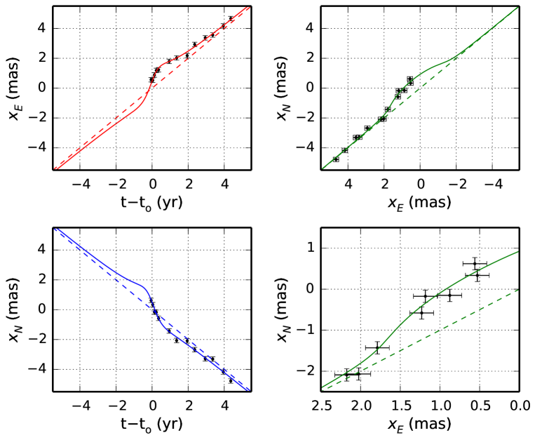
Figure 18.— A simulation of the 2D astrometric shift due a 10-M_⊙ black hole at 4 kpc microlensing a background source at 8 kpc with a relative proper motion of 7 mas yr^-1 and impact parameter $u_{0}$ = 0.5. The model X (top left) and Y (bottom left) positions vs. time are shown (solid) overlaid with simulated astrometric measurements and an unlensed source motion (dashed). The measurements on the plane of the sky are shown in the top right and zoomed in on the bottom right. Error bars represent the 1$\sigma$ astrometric uncertainty expected from NIRC2 observations (0.15 mas). The astrometric effects of parallax have been omitted.

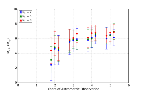
Figure 19.— 3$\sigma$ lower limits for lens mass ($M_{\mathrm{min}}$) recovered from different simulated observing strategies assuming a 10-M_⊙ lens at 4 kpc, and a source at 8 kpc. Colors distinguish the number of nights of observations in year 1 ($N_{1}$) as labeled in the legend. The horizontal axis indicates the total number of years of observation ($N_{\mathrm{yrs}}$). For each value of $N_{\mathrm{yrs}}>1$ there are three columns, corresponding to (left-to-right) 1, 2, and 3 observations per year after year 1 ($N_{>1}$). The $M_{\mathrm{min}}$ values plotted for each observing strategy indicate the median of 100 trials, with 1-$\sigma$ error bars. The dashed line indicates 5 M_⊙—the minimum mass that we assume is required to confidently conclude a BH.

Within this margin of error, none of the two-year observing strategies confirm $M>5$ M_⊙ with 3$\sigma$ confidence. A minimum $N_{\mathrm{yrs}}=3$ is required. There is significant improvement when $N_{\mathrm{yrs}}$ increases from two to three, but further increases have minimal and diminishing returns. Figure 18 shows that astrometric measurements both two and three years after the event peak adequately constrain the unlensed proper motion. Strategies with $N_{>1}\geq 2$ are recommended to protect against single measurement outliers. Adopting $N_{1}>2$ marginally improves mass constraints, but it does not seem to be necessary. Still, we recommend $N_{1}\geq 3$ to protect against single measurement outliers. In summary, we conclude that future searches for isolated BHs should adopt an observing strategy with $N_{1}\geq 3$, $N_{>1}\geq 2$, and $N_{\mathrm{yrs}}\geq 3$.

Finally, our use of photometry to identify candidate long-duration events for astrometric follow-up might favor binary lenses, which must be considered in future target selection. In principle, a goodness of fit comparison of the single-lens and multiple-lens models before astrometric follow-up might be a viable screening option. Unfortunately, the primary factor distinguishing these models is the degree of symmetry in the light curve around the peak. Therefore, it is unlikely that the lens multiplicity can be constrained before astrometric follow-up begins (i.e. before or near the peak). Exceptions include caustic crossing events for which finite-source effects appear before the event peak.

9. Conclusions

While stellar mass black holes still remain elusive, this study demonstrates the feasibility of detecting them in the near future, and provides a strategy to do so efficiently based on demonstrated astrometric and photometric precision. This is the first study that uses both astrometric and photometric ground-based measurements to constrain lensing event parameters. The value of a precise measurement of the proper motion of the source or the combined source-lens system is demonstrated in the tight upper limit on the mass of OB110022, which we show is not a black hole. Moreover, by uncovering and mitigating Keck/NIRC2 systematic effects like spatial variation of the PSF, and exploring the effects of using different transformations in cross-epoch alignment, this study informs future analysis of any astrometric data, regardless of the scientific motivation. Follow-up astrometric observations of one of our targets, OB120169, should further constrain mass of the lens, which could be a black hole. Very few studies have attempted the astrometric detection of stellar mass black holes, but it seems a worthwhile endeavor.

10. Acknowledgements

The authors would like to thank Subo Dong (Kavli Institute for Astronomy and Astrophysics, Peking University) for his significant contributions to this work. J.R.L. acknowledges support for this work from the California Institute of Technology Millikan Postdoctoral Fellow program and the NSF Astronomy and Astrophysics Postdoctoral Fellow program (AST−1102791). E.O.O. is an incumbent of the Arye Dissentshik career development chair and is grateful for support by grants from the Willner Family Leadership Institute Ilan Gluzman (Secaucus NJ), Israel Science Foundation, Minerva, Weizmann-UK, and the I-Core program by the Israeli Committee for Planning and Budgeting and the Israel Science Foundation (ISF). The OGLE project has received funding from the National Science Centre, Pland, grant MAESTRO 2014/14/A/ST9/00121 to AU. E.S. acknowledges the SWOOP writing retreat and its participants for useful feedback. The data presented herein were obtained at the W. M. Keck Observatory, which is operated as a scientific partnership among the California Institute of Technology, the University of California and the National Aeronautics and Space Administration. The Observatory was made possible by the generous financial support of the W. M. Keck Foundation. The authors wish to recognize and acknowledge the very significant cultural role and reverence that the summit of Mauna Kea has always had within the indigenous Hawaiian community. We are most fortunate to have the opportunity to conduct observations from this mountain.

Appendix A A. Weighting Schemes in Cross-Epoch Alignment

We experimented with four different weighting schemes to apply to the sources used to derive the cross-epoch transformation. We tried applying weights for each star in each epoch, $i$, given by,

1. $W_{i}=1$

2. $W_{i}=1/\sigma_{i}^{2}$

3. $W_{i}=1/\sqrt{\sigma_{i}^{2}+\sigma_{0}^{2}+(\sigma_{\mu}[t-t_{0}])^{2}}$

4. $W_{i}=1/\left[\sigma_{i}^{2}+\sigma_{0}^{2}+(\sigma_{\mu}[t-t_{0}])^{2}\right]$

where $\sigma_{i}$ is a star’s positional uncertainty in epoch $i$, $\sigma_{0}$ is the positional uncertainty in the reference epoch (April 2013), $\sigma_{\mu}$ is its proper motion uncertainty and $t-t_{0}$ is the time between the reference epoch and epoch of interest. Including $\sigma_{0}$ and $\sigma_{\mu}(t-t_{0})$ incorporates the fact that, since all coordinate systems are aligned to the reference epoch, the positional uncertainty grows with time from that epoch in proportion to the source velocity. We applied these weights averaged over $x$ and $y$. These four weighting schemes are hereafter denoted W1, W2, W3 and W4 respectively. W3 and W4 incorporate positional uncertainties associated with time from the reference epoch. W3 results in a weighting that is less sensitive to differences in uncertainty than W4.

Figure 20 shows the distribution of position residuals obtained using the four different weighting schemes for OB110022, normalized by the positional uncertainy, $\sigma_{pos}$. Their consistency suggests that our particular choice of weighting scheme does not affect the precision of the proper motion fit. However, we must still ensure that its accuracy is also invariant of the weighting scheme. Even if the choice of weighting scheme does not influence the error of the proper motion fit it could still affect the best fit value. To test this we obtain the difference distribution $\delta$ of the proper motion measurements for each source $q$ under weighting scheme $p$ versus a different weighting scheme $k$ and check that it is consistent with the errors on each proper motion measurement. Specifically,

$$\delta_{q,p,k}=\frac{\mu_{q,p}-\mu_{q,k}}{\left(\sigma_{\mu_{q,p}}^{2}+\sigma_{\mu_{q,k}}^{2}\right)^{1/2}},$$ (A1)

for all stars $q$, where $p\neq k$. Figure 21 shows the resulting distributions obtained in both x and y. Given the apparent consistencies of both this proper motion difference distribution and the position residuals distributions with their associated errors, we conclude that the our particular choice of weighting scheme will not affect our results. Therefore, we arbitrarily elected to use W4, which is the statistically appropriate weighting scheme when errors are normally distributed and well characterized.

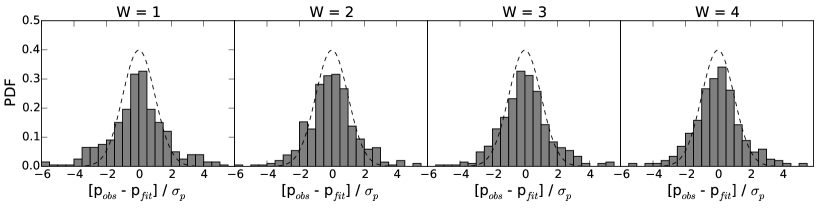
(a) W1

Figure 20.— Histogram of residuals to the proper motion fits for all stars in the OB110022 epochs, using the four different cross-epoch alignment weighting schemes. The residuals are normalized by the positional uncertainties. Their mutual Gaussian shape indicates that the choice of weighting scheme does not affect the errors on the transformations and proper motion fits.

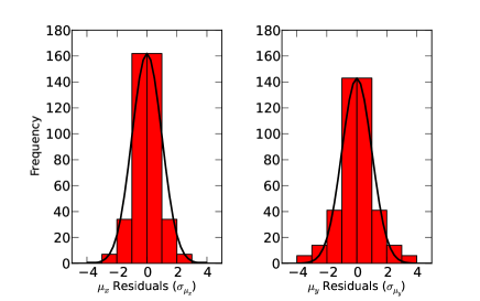
Figure 21.— Distribution of the difference between proper motion measurements of each star in the OB110022 field across different cross-epoch alignment weighting schemes, in units of their associated error. The Gaussian distribution indicates that the derived proper motions are independent of weighting scheme.

Appendix B B. Transformation Order in Cross-Epoch Alignment

We tested cross-epoch transformations of order O$=$1, 2, and 3 in a manner similar to Clarkson et al. (2012). For each order, we define the metric $\chi_{aln,vel}^{2}$(O), as a means of quantifing the goodness-of-fit for the combined transformation fits and proper motion fits for all stars over all epochs. We sum the residuals between the observed position, after transformation, and the predicted position from the best-fit proper motion for all epochs and all stars in each target’s field:

$$\chi_{aln,vel}^{2}=\sum_{s}^{N_{\mathrm{stars}}}\sum_{e}^{N_{\mathrm{epochs}}}\left[\frac{x_{\mathrm{obs,s,e}}-x_{\mathrm{fit,s,e}}}{\sigma_{\mathrm{x,s,e}}}\right]^{2}+\left[\frac{y_{\mathrm{obs,s,e}}-y_{\mathrm{fit,s,e}}}{\sigma_{\mathrm{y,s,e}}}\right]^{2}$$ (B1)

where $\sigma_{\mathrm{x,s,e}}$ and $\sigma_{\mathrm{y,s,e}}$ include only the positional errors, $\sigma_{\mathrm{p}}$, and do not include the alignment errors. The number of degrees of freedom (DOF) for the combined alignment and velocity fits is the difference between $N_{\mathrm{data}}$, the total number of positional measurements, and $N_{\mathrm{par}}$, the number of free parameters including those from the transformation for each epoch and the proper motion fits for all stars in the field of view (Table 9). For increasing model complexity (i.e. polynomial order), we evaluated the change in $\chi_{aln,vel}^{2}$ using the F-ratio,

$$F=\left(\frac{\chi^{2}(O-1)-\chi^{2}(O)}{\chi^{2}(O)}\right)\frac{N_{\mathrm{data}}-N_{\mathrm{par}}(O)}{N_{\mathrm{par}}(O)-N_{\mathrm{par}}(O-1)}.$$ (B2)

Table 9 gives the resulting $\chi_{aln,vel}^{2}$ values for each order, the F-ratios when increasing from $O-1\rightarrow O$, and the p-value, which is the probability of obtaining this F-ratio, or higher, from chance. Lower p-values indicate more significant benefits to increasing the order of the transformation polynomials. We note that the $\chi_{aln,vel}^{2}$ values are high relative to the degrees of freedom, which typically suggests that uncertainties should be re-scaled to larger values. However, the F-ratio is insensitive to error re-scaling and can still be used to select the optimal order of the transformation. For OB110022, the $\chi_{aln,vel}^{2}$ values in Table 9 increase for higher-order fits, which may be caused either by instability of the high-order fit, given the small number of epochs, or a high condition number in the inversion. Furthermore, $\chi_{aln,vel}^{2}$ values do not include the transformation uncertainties and should not be interpreted as the final quality of our astrometric transformations and proper motion fits. OB110022 showed no significant improvement when advancing to 2nd order (F-ratio$<$1), therefore we adopt O$=$1 for this source. Both OB110125 and OB120169 showed marginal improvement going from O$=1\rightarrow 2$ and the $\chi^{2}$ distribution for O$=$2 showed significant improvement, therefore we adopted O$=$2 for these sources.

Figure 22 shows the distribution of residuals for all stars in all epochs for each target field and each transformation order and Figure 23 shows the distribution of $\chi_{vel}^{2}$ for each stars proper motion fit (i.e. weighted residuals summed over $N_{epochs}$). Note that these $\chi_{vel}^{2}$ values do not include the alignment error; but, are the individual values (one for each star) that go into the F-ratio. Again, the relative improvement is most significant for O$=1\rightarrow 2$ for OB120169 and OB110125. Note that these distributions of residuals and $\chi_{vel}^{2}$ values are only used to judge the choice of transformation order and are not final as they do not include the uncertainties in the transformation process. For completeness, the distribution of residuals and $\chi_{vel}^{2}$ values including both the positional and alignment errors are shown in Figures 24 and 25 for all three targets and all three transformation orders.

Finally, the microlensing fits were run for O$=$1 and O$=$2 for OB110022 and OB120169 and there was a negligable change in the final lens-mass posteriors of less than $<$0.1 M${}_{\odot}~{}$for all limits.

Table 9F-ratio for Alignment Order

						Order
Source	Order	$\chi_{aln,vel}^{2}$	Ndata	Npar	DOFaln,vel	Change	F-ratio	p-value
OB110022	O$=1$	1023	408	166	242
	O$=2$	1156	408	196	212	O$=1\rightarrow 2$	-0.81	1.0000
	O$=3$	2487	408	236	172	O$=2\rightarrow 3$	-2.30	1.0000
OB110125	O$=1$	2784	500	224	276
	O$=2$	1995	500	248	252	O$=1\rightarrow 2$	4.15	0.0000
	O$=3$	1810	500	280	220	O$=2\rightarrow 3$	0.70	0.8822
OB120169	O$=1$	1277	210	108	102
	O$=2$	926	210	132	78	O$=1\rightarrow 2$	1.23	0.2403
	O$=3$	787	210	164	46	O$=2\rightarrow 3$	0.25	0.9999

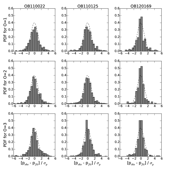
Figure 22.— Histogram of error-weighted residuals to the linear source proper motion fits, $(p_{obs}-p_{fit})/\sigma$, for all three targets and different transformation orders, O=1, 2, 3. The errors include only positional errors, $\sigma_{p}$. Residuals for both X and Y are included. The resulting distribution of residuals are largely consistent with with a normal distribution with a 1$\sigma$ spread for all orders (black dashed line). Note the final analysis uses O=1 for OB110022 and O=2 for OB110125 and OB120169.

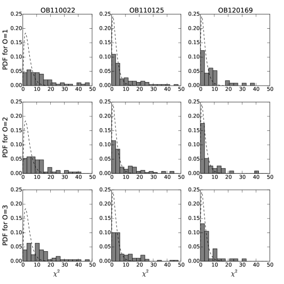
Figure 23.— Histogram of $\chi^{2}$ values of each star’s proper motion fit for all three targets and different transformation orders, O=1, 2, 3. The $\chi^{2}$ values for both X and Y are included in the histogram and the degrees of freedom for the expected $\chi^{2}$ distribution (black dashed line) is given by the number of epochs of data - 2 free parameters in the velocity fit. Only positional errors, $\sigma_{p}$, were included. The F-test used to evaluate the transformation order sums these $\chi^{2}$ values over the number of stars and X and Y and the final degrees of freedom is modified to include the transformation parameters for each epoch of data. OB110125 and OB120169 show statistically significant improvements in the $\chi^{2}$ distribution relative to the expectation when going from O$=1\rightarrow 2$.

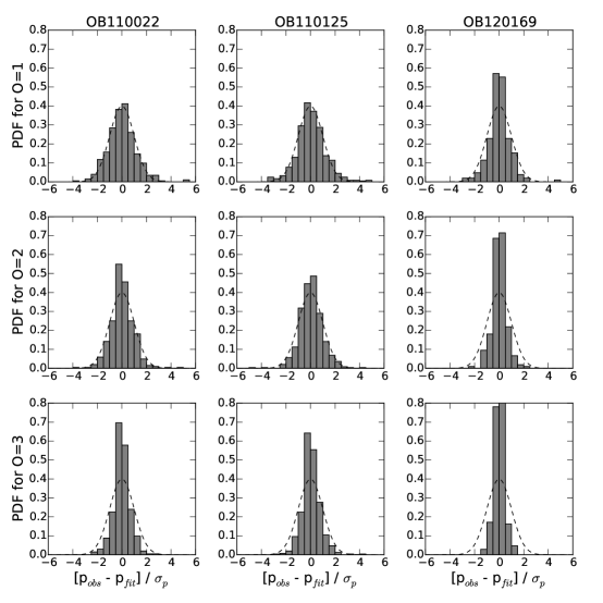
Figure 24.— Identical to Figure 22 only the errors include both positional and alignment errors, $\sigma=\sqrt{\sigma_{p}^{2}+\sigma_{a}^{2}}$. The resulting width of the residuals decreases with increasing transformation order as the alignment errors increases.

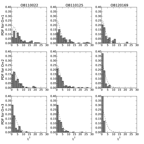
Figure 25.— Identical to Figure 23 only the errors include both positional and alignment errors, $\sigma=\sqrt{\sigma_{p}^{2}+\sigma_{a}^{2}}$. The resulting $\chi^{2}$ distribution shows only slight changes for OB110022 with increasing transformation order. OB110125 and OB120169 show more dramatic improvements when changing from O$=1\rightarrow 2$.

References

- Abbott et al. (2009) Abbott, B. P., et al. 2009, Reports on Progress in Physics, 72, 076901
- Agol & Kamionkowski (2002) Agol, E., & Kamionkowski, M. 2002, MNRAS, 334, 553
- Albrow et al. (2000) Albrow, M. D., et al. 2000, ApJ, 534, 894
- Alcock et al. (1995) Alcock, C., et al. 1995, ApJ, 454, L125
- Alcock et al. (1997) —. 1997, ApJ, 491, 436
- Alcock et al. (2001) —. 2001, Nature, 414, 617
- An et al. (2002) An, J. H., et al. 2002, ApJ, 572, 521
- Babu & Feigelson (1996) Babu, G. J., & Feigelson, E. D. 1996, Astrostatistics
- Batista et al. (2015) Batista, V., Beaulieu, J.-P., Bennett, D. P., Gould, A., Marquette, J.-B., Fukui, A., & Bhattacharya, A. 2015, ApJ, 808, 170
- Bennett et al. (2002) Bennett, D. P., et al. 2002, ApJ, 579, 639
- Boden et al. (1998) Boden, A. F., Shao, M., & Van Buren, D. 1998, ApJ, 502, 538
- Bond (2001) Bond, I. 2001, in Cosmological Physics with Gravitational Lensing, ed. J. Tran Thanh Van, Y. Mellier, & M. Moniez, 11–18
- Britton (2006) Britton, M. C. 2006, PASP, 118, 885
- Calchi Novati et al. (2015) Calchi Novati, S., et al. 2015, ApJ, 804, 20
- Casares & Jonker (2014) Casares, J., & Jonker, P. G. 2014, Space Sci. Rev., 183, 223
- Choi et al. (2012) Choi, J.-Y., et al. 2012, ApJ, 751, 41
- Clarkson et al. (2012) Clarkson, W. I., Ghez, A. M., Morris, M. R., Lu, J. R., Stolte, A., McCrady, N., Do, T., & Yelda, S. 2012, ApJ, 751, 132
- Delplancke et al. (2001) Delplancke, F., Górski, K. M., & Richichi, A. 2001, A&A, 375, 701
- Diolaiti et al. (2000) Diolaiti, E., Bendinelli, O., Bonaccini, D., Close, L., Currie, D., & Parmeggiani, G. 2000, The Messenger, 100, 23
- Dominik (1999) Dominik, M. 1999, A&A, 349, 108
- Dong et al. (2007) Dong, S., et al. 2007, ApJ, 664, 862
- Feroz et al. (2009) Feroz, F., Hobson, M. P., & Bridges, M. 2009, MNRAS, 398, 1601
- Feroz et al. (2013) Feroz, F., Hobson, M. P., Cameron, E., & Pettitt, A. N. 2013, arXiv:1306.2144
- Fitzgerald et al. (2012) Fitzgerald, M. P., et al. 2012, in Proc. SPIE, Vol. 8447, Adaptive Optics Systems III, 844724
- Fruchter & Hook (2002) Fruchter, A. S., & Hook, R. N. 2002, PASP, 114, 144
- Ghez et al. (2000) Ghez, A. M., Morris, M., Becklin, E. E., Tanner, A., & Kremenek, T. 2000, Nature, 407, 349
- Ghez et al. (2005) Ghez, A. M., Salim, S., Hornstein, S. D., Tanner, A., Lu, J. R., Morris, M., Becklin, E. E., & Duchêne, G. 2005, ApJ, 620, 744
- Girardi et al. (2012) Girardi, L., et al. 2012, TRILEGAL, a TRIdimensional modeL of thE GALaxy: Status and Future, ed. A. Miglio, J. Montalbán, & A. Noels, 165
- Gould (1992) Gould, A. 1992, ApJ, 392, 442
- Gould (1994a) —. 1994a, ApJ, 421, L75
- Gould (1994b) —. 1994b, ApJ, 421, L71
- Gould (2000) —. 2000, ApJ, 535, 928
- Gould (2004) —. 2004, ApJ, 606, 319
- Gould & Salim (2002) Gould, A., & Salim, S. 2002, ApJ, 572, 944
- Gould & Yee (2014) Gould, A., & Yee, J. C. 2014, ApJ, 784, 64
- Gould et al. (2009) Gould, A., et al. 2009, ApJ, 698, L147
- Gubler & Tytler (1998) Gubler, J., & Tytler, D. 1998, PASP, 110, 738
- Han & Chang (2000) Han, C., & Chang, K. 2000, ArXiv Astrophysics e-prints
- Han & Jeong (1999) Han, C., & Jeong, Y. 1999, MNRAS, 309, 404
- Hog et al. (1995) Hog, E., Novikov, I. D., & Polnarev, A. G. 1995, A&A, 294, 287
- Jeong et al. (1999) Jeong, Y., Han, C., & Park, S.-H. 1999, ApJ, 511, 569
- Jung et al. (2015) Jung, Y. K., et al. 2015, ApJ, 798, 123
- Kochanek et al. (2008) Kochanek, C. S., Beacom, J. F., Kistler, M. D., Prieto, J. L., Stanek, K. Z., Thompson, T. A., & Yüksel, H. 2008, ApJ, 684, 1336
- Kozłowski et al. (2007) Kozłowski, S., Woźniak, P. R., Mao, S., & Wood, A. 2007, ApJ, 671, 420
- Kushnir (2015) Kushnir, D. 2015, ArXiv e-prints
- Kushnir & Katz (2015) Kushnir, D., & Katz, B. 2015, ApJ, 811, 97
- Lu et al. (2009) Lu, J. R., Ghez, A. M., Hornstein, S. D., Morris, M. R., Becklin, E. E., & Matthews, K. 2009, ApJ, 690, 1463
- Lu et al. (2010) Lu, J. R., Ghez, A. M., Yelda, S., Do, T., Clarkson, W., McCrady, N., & Morris, M. 2010, in Society of Photo-Optical Instrumentation Engineers (SPIE) Conference Series, Vol. 7736, Society of Photo-Optical Instrumentation Engineers (SPIE) Conference Series
- Mao et al. (2002) Mao, S., et al. 2002, MNRAS, 329, 349
- Miyamoto & Yoshii (1995) Miyamoto, M., & Yoshii, Y. 1995, AJ, 110, 1427
- Paczynski (1986) Paczynski, B. 1986, ApJ, 301, 503
- Paczyński & Stanek (1998) Paczyński, B., & Stanek, K. Z. 1998, ApJ, 494, L219
- Park et al. (2013) Park, H., et al. 2013, ApJ, 778, 134
- Park et al. (2015) —. 2015, ApJ, 805, 117
- Pejcha & Prieto (2015) Pejcha, O., & Prieto, J. L. 2015, ApJ, 806, 225
- Poindexter et al. (2005) Poindexter, S., Afonso, C., Bennett, D. P., Glicenstein, J.-F., Gould, A., Szymański, M. K., & Udalski, A. 2005, ApJ, 633, 914
- Prince et al. (2007) Prince, T., et al. 2007, LISA: Probing the Universe with Gravitational Waves, Executive Summary, http://lisa.nasa.gov/Documentation/LISA-LIST-RP-436v1.2.pdf
- Reynolds & Miller (2013) Reynolds, M. T., & Miller, J. M. 2013, ApJ, 769, 16
- Sajadian (2014) Sajadian, S. 2014, MNRAS, 439, 3007
- Shvartzvald et al. (2015) Shvartzvald, Y., et al. 2015, ArXiv e-prints
- Skilling (2006) Skilling, J. 2006, Bayesian Anal., 1, 833
- Skrutskie et al. (2006) Skrutskie, M. F., et al. 2006, AJ, 131, 1163
- Smith et al. (2003) Smith, M. C., Mao, S., & Paczyński, B. 2003, MNRAS, 339, 925
- Stolte et al. (2008) Stolte, A., Ghez, A. M., Morris, M., Lu, J. R., Brandner, W., & Matthews, K. 2008, ApJ, 675, 1278
- Szymański et al. (2000) Szymański, M., Udalski, A., Kubiak, M., Pietrzyński, G., Soszyński, I., Woźniak, P., & Zebruń, K. 2000, in Astronomische Gesellschaft Meeting Abstracts, Vol. 16, Astronomische Gesellschaft Meeting Abstracts, ed. R. E. Schielicke, 19
- Udalski (2003) Udalski, A. 2003, Acta Astron., 53, 291
- Udalski et al. (1992) Udalski, A., Szymanski, M., Kaluzny, J., Kubiak, M., & Mateo, M. 1992, Acta Astron., 42, 253
- Udalski et al. (2015a) Udalski, A., Szymański, M. K., & Szymański, G. 2015a, Acta Astron., 65, 1
- Udalski et al. (2015b) Udalski, A., et al. 2015b, ApJ, 799, 237
- van Dam et al. (2006) van Dam, M. A., et al. 2006, PASP, 118, 310
- Walker (1995) Walker, M. A. 1995, ApJ, 453, 37
- Witt & Mao (1994) Witt, H. J., & Mao, S. 1994, ApJ, 430, 505
- Wizinowich et al. (2006) Wizinowich, P. L., et al. 2006, PASP, 118, 297
- Wozniak (2000) Wozniak, P. R. 2000, Acta Astron., 50, 421
- Wyrzykowski et al. (2015) Wyrzykowski, L., et al. 2015, ArXiv e-prints
- Yee et al. (2009) Yee, J. C., et al. 2009, ApJ, 703, 2082
- Yee et al. (2015) —. 2015, ApJ, 802, 76
- Yelda et al. (2010) Yelda, S., Lu, J. R., Ghez, A. M., Clarkson, W., Anderson, J., Do, T., & Matthews, K. 2010, ApJ, 725, 331
- Yoo et al. (2004) Yoo, J., et al. 2004, ApJ, 603, 139
- Zhu et al. (2015) Zhu, W., et al. 2015, ApJ, 805, 8
- Zub et al. (2011) Zub, M., et al. 2011, A&A, 525, A15