Frequency dispersion of small-amplitude capillary waves in viscous fluids

Abstract

This work presents a detailed study of the dispersion of capillary waves with small amplitude in viscous fluids using an analytically derived solution to the initial value problem of a small-amplitude capillary wave as well as direct numerical simulation. A rational parametrization for the dispersion of capillary waves in the underdamped regime is proposed, including predictions for the wavenumber of critical damping based on a harmonic oscillator model. The scaling resulting from this parametrization leads to a self-similar solution of the frequency dispersion of capillary waves that covers the entire underdamped regime, which allows an accurate evaluation of the frequency at a given wavenumber, irrespective of the fluid properties. This similarity also reveals characteristic features of capillary waves, for instance that critical damping occurs when the characteristic timescales of dispersive and dissipative mechanisms are balanced. In addition, the presented results suggest that the widely adopted hydrodynamic theory for damped capillary waves does not accurately predict the dispersion when viscous damping is significant and a new definition of the damping rate, which provides consistent accuracy in the underdamped regime, is presented.

I Introduction

Waves at fluid interfaces are ubiquitous in two-phase flows across a wide range of scales, from the tidal wave with a wavelength of $\lambda\sim 10^{7}\,\mathrm{m}$ and tsunamis ($\lambda>10^{5}\,\mathrm{m}$) down to wavelengths of the order of the size of individual molecules. For interfacial waves with long wavelength, $\lambda\gg\sqrt{\sigma/(\rho g)}$ (where $\sigma$ is the surface tension coefficient, $\rho$ is the fluid density and $g$ is the gravitational acceleration), so-called gravity waves, gravity is the main mechanism governing these waves, whereas for interfacial waves with small wavelength, $\lambda\ll\sqrt{\sigma/(\rho g)}$, so-called capillary waves, surface tension is the dominant dispersive and restoring mechanism. In addition, viscous stresses act preferably at small scales (Lamb, 1932), leading to an increasing viscous attenuation of capillary waves with decreasing wavelength and a decreasing frequency of capillary waves for increasing viscosity (Levich, 1962). Longuet-Higgins (1992) elegantly summarized the governing mechanisms for capillary waves: “At small scales, the role of surface tension and viscosity are all-important”.

Capillary waves play an important role in the capillary-driven breakup (Rayleigh-Plateau instability) of liquid jets and ligaments (Eggers and Villermaux, 2008; Castrejón-Pita et al., 2015), the atomization of liquid jets (Tsai et al., 1997) as well as the stability of liquid and capillary bridges (Hoepffner and Paré, 2013) and of liquid curtains (Lhuissier et al., 2016). Capillary waves are observed at the front of short gravity waves (Longuet-Higgins, 1963; Longuet-Higgins and Stewart, 1964; Longuet-Higgins, 1995; Crapper, 1970), for instance in the ocean where they enhance the heat and mass transfer between water and atmosphere (Witting, 1971; Szeri, 1997). Capillary waves have also been identified as the key mechanism governing the formation of bound states of solitary waves in falling liquid films (Pradas et al., 2011) and have been observed to enhance film thinning between two approaching interfaces, for instance in foams and emulsions (Ruckenstein and Sharma, 1987). Shats et al. (2010) observed the formation of capillary rogue waves in experiments, meaning capillary waves can serve as a prototype to study the formation of rogue waves in a relatively easily accessible laboratory experiment. Similarly, capillary waves are used to study wave turbulence experimentally (Falcon et al., 2007; Xia et al., 2010; Deike et al., 2012) as well as numerically (Pushkarev and Zakharov, 1996; Deike et al., 2014a). In cell biology, capillary waves influence the behavior and properties of lipid membranes, micelles and vesicles (Crawford and Earnshaw, 1987; Lebedev and Muratov, 1989; Gompper and Kroll, 1992), and with respect to microfluidic applications, capillary waves are of central interest to applications such as surface wave acoustics (Yeo and Friend, 2014), microstreaming (Chindam et al., 2013) and ultrasound cavitation (Tandiono et al., 2010).

Since capillary waves inherently have a short wavelength, understanding the physical processes and optimizing the engineering applications named in the examples above are dependent, among others, on a detailed knowledge of the influence of viscous stresses on capillary waves. For instance, viscosity reduces the growth rate of the Rayleigh-Plateau instability in liquid jets (Weber, 1931; Chandrasekhar, 1961) and alters the size, number and speed of capillary waves in between interacting solitary waves on falling liquid films (Kalliadasis et al., 2012; Dietze, 2016; Denner et al., 2016). Due to the significantly higher dissipation of capillary waves compared to gravity waves, capillary waves occurring on the forward facing slope of gravity waves are the main means of dissipation for gravity waves (Longuet-Higgins and Stewart, 1964; Longuet-Higgins, 1992, 1995; Sajjadi, 2002; Melville and Fedorov, 2015). The dissipation of capillary waves has also been found to increase sharply with increasing steepness of gravity waves, thus delaying the breaking of gravity waves (Longuet-Higgins, 1963; Crapper, 1970; Deike et al., 2015; Melville and Fedorov, 2015). Viscosity plays an important role in the energy transfer across scales in capillary wave turbulence (Deike et al., 2012, 2014b; Abdurakhimov et al., 2015; Haudin et al., 2016) and has also been suggested to be the main reason for the bi-directional energy cascade observed in capillary wave turbulence (Abdurakhimov et al., 2015). For instance, Deike et al. (2014b) showed that the steepness of the power-law spectrum of capillary wave turbulence increases with increasing viscosity. Perrard et al. (2015) studied the propagation of capillary solitons on a levitated body of liquid and found viscous dissipation to be responsible for a gradual decrease in wave amplitude, which in turn affects the phase velocity and leads to a turbulence-like regime at high frequency with respect to the amplitude power-spectrum. Capillary waves considerably influence the behavior and properties, e.g. glass transition temperature and effective viscosity, of viscoelastic materials (Monroy and Langevin, 1998; Harden et al., 1991; Herminghaus, 2002; Herminghaus et al., 2004), such as gels and polymers, with critical damping marking the transition between inelastic and quasielastic behavior (Harden et al., 1991; Madsen et al., 2004).

In an inviscid, ideal fluid the angular frequency of capillary waves is given as (Lamb, 1932)

$$\omega_{0}=\sqrt{\frac{\sigma k^{3}}{\tilde{\rho}}}\ ,$$ (1)

where $\sigma$ is the surface tension coefficient, $k=2\pi/\lambda$ is the wavenumber and $\tilde{\rho}=\rho_{\mathrm{a}}+\rho_{\mathrm{b}}$ is the relevant fluid density, where subscripts $\mathrm{a}$ and $\mathrm{b}$ denote properties of the two interacting bulk phases. Thus, the frequency as well as the phase velocity $c_{0}=\omega_{0}/k$ of capillary waves in inviscid fluids increase with increasing wavenumber, with $\omega_{0}\rightarrow\infty$ for $k\rightarrow\infty$.

In viscous fluids, viscous stresses attenuate the wave motion and the frequency takes on the complex form $\omega=\omega_{0}+i\Gamma$, with a single frequency for each wavenumber (Jeng et al., 1998). Three distinct damping regimes can be identified for capillary waves in viscous fluids (similar to other damped oscillators): the underdamped regime for $k<k_{\mathrm{c}}$, critical damping for $k=k_{\mathrm{c}}$ and the overdamped regime for $k>k_{\mathrm{c}}$. At critical damping, with critical wavenumber $k_{\mathrm{c}}$, the wave requires the shortest time to return to its equilibrium state without oscillating, meaning that the real part of the complex angular frequency is $\mathrm{Re}(\omega)=0$. Critical damping, hence, represents the transition from the underdamped (oscillatory) regime, with $k<k_{\mathrm{c}}$ and $\mathrm{Re}(\omega)>0$, to the overdamped regime, with $\mathrm{Re}(\omega)=0$ and $k>k_{\mathrm{c}}$. Based on the linearized Navier-Stokes equations, the dispersion relation of capillary waves in viscous fluids is given as (Landau and Lifshitz, 1966; Levich, 1962; Byrne and Earnshaw, 1979; Earnshaw and Hughes, 1991)

$$\omega_{0}^{2}+\left(i\omega+2\nu k^{2}\right)^{2}-4\nu^{2}k^{4}\sqrt{1+\frac{i\omega}{\nu k^{2}}}=0\ ,$$ (2)

where $\nu=\mu/\rho$ is the kinematic viscosity and $\mu$ is the dynamic viscosity. From Eq. (2) the damping rate follows as $\Gamma=2\nu k^{2}$. This damping rate is valid in the weak damping regime, for $k\ll\sqrt{\omega_{0}/\nu}$, where viscous damping is considered to be small (Levich, 1962; Jeng et al., 1998).

Most research to date has focused on linear wave theory under the assumption of inviscid fluids or based on the linearized Navier-Stokes equations (weak damping). These assumptions have significant limitations with respect to capillary waves with short wavelength, for which viscous attenuation is a dominant influence. The inviscid assumption is only valid for long waves where viscous damping is negligible, whereas the weak damping assumption is valid when viscous stresses have a small effect on the dispersion of capillary waves (Lamb, 1932; Levich, 1962; Jeng et al., 1998). Furthermore, the damping rate $\Gamma$ is not a constant value, as presupposed by the weak damping assumption, but changes considerably throughout the underdamped regime (Jeng et al., 1998). Similarly, the linearized Navier-Stokes equations assume that nonlinear effects are negligible, which is not the case for short capillary waves or highly viscous fluids (Behroozi et al., 2011). As a result, a rational parametrization and consistent characterization that accurately describes the frequency dispersion of capillary waves in viscous fluids is not available to date.

The goal of this study is the formulation of a rational parametrization of the dispersion of capillary waves in viscous fluids, which is valid throughout the entire underdamped regime and for two-phase systems with arbitrary fluid properties. To this end, the dispersion and oscillatory behavior of capillary waves is studied from a purely hydrodynamic perspective based on continuum mechanics, assuming that continuum mechanics is valid in the entire underdamped regime, including critical damping, as previously shown by Delgado-Buscalioni et al. (2008). The dispersion of capillary waves with small amplitude in different viscous fluids is computed using an analytical initial-value solution (AIVS) as well as direct numerical simulation (DNS). Given the validity of the underpinning assumptions, AIVS is used for capillary waves in one-phase systems (i.e. a single fluid with a free surface) as well as two-phase systems in which both phases have the same kinematic viscosity $\nu$, whereas DNS is applied to extend the study to arbitrary fluid properties.

A harmonic oscillator model for capillary waves is proposed, which accurately predicts the wavenumber $k_{\mathrm{c}}$ at which a capillary wave in arbitrary viscous fluids is critically damped, and a consistent scaling for capillary waves is derived from rational arguments. Based on this scaling as well as the critical wavenumber predicted by the harmonic oscillator model, a self-similar characterization of the frequency dispersion of capillary waves in viscous fluids is introduced. This characterization allows an accurate a priori evaluation of the frequency of capillary waves for two-phase systems with arbitrary fluid properties, and unveils distinct features of capillary waves that are independent of the fluid properties. Moreover, different methods to predict the frequency of capillary waves are studied and a new definition of the effective damping rate is proposed, which provides a more accurate frequency prediction than commonly used definitions when viscous stresses dominate.

In Sec. II the characterization of capillary waves is discussed and Sec. III introduces the applied computational methods. Section IV examines critical damping and proposes a harmonic oscillator model to parameterize capillary waves. Section V analyses and discusses the similarity of the frequency dispersion of capillary waves and Sec. VI examines different damping assumptions and frequency estimates. The article is summarised and conclusions are drawn in Sec. VII.

II Characterization of capillary waves

Two physical mechanisms govern the oscillatory motion of capillary waves: surface tension, which is the dominant dispersive and restoring mechanism, and viscous stresses in the fluids, which is the prevailing dissipative mechanism . Other physical mechanisms, such as inertia or gradients in surface tension coefficient, can be neglected, since no external forces (e.g. gravity) are imposed on the fluids or the interface, the fluids are considered pure (i.e. free of surfactants), and the fluid motion induced by the small-amplitude capillary waves is dominated by viscosity (i.e. creeping flow).

Capillary (surface tension) effects are quantified by their characteristic pressure $p_{\sigma}={\sigma}/{l}$, where $l$ is a reference lengthscale, and their characteristic timescale $t_{\sigma}=\sqrt{{\tilde{\rho}\,l^{3}}/{\sigma}}$, which is proportional to the undamped period of a capillary wave (with $t_{\sigma}=\omega_{0}^{-1}$ for $l=k^{-1}$). With respect to viscous stresses, the characteristic pressure is $p_{\mu}={\tilde{\mu}\,u}/{l}$, where $\tilde{\mu}=\mu_{\mathrm{a}}+\mu_{\mathrm{b}}$ and $u$ is a reference velocity. The characteristic timescale associated with viscous stresses, which is representative of the time required for momentum to diffuse through a distance $l$, is $t_{\mu}={\tilde{\rho}\,l^{2}}/{\tilde{\mu}}$. Quantifying the relative importance of surface tension and viscous stresses, the characteristic pressures lead to the capillary number

$$\mathrm{Ca}=\frac{p_{\mu}}{p_{\sigma}}=\frac{\tilde{\mu}\,u}{\sigma}$$ (3)

and the ratio of the characteristic timescales is given by the Ohnesorge number

$$\mathrm{Oh}=\frac{t_{\sigma}}{t_{\mu}}=\frac{\tilde{\mu}}{\sqrt{\sigma\,\tilde{\rho}\,l}}\ .$$ (4)

Assuming that surface tension and viscous stresses are equally important, the viscocapillary velocity follows from $\mathrm{Ca}=1$ as

$$u_{\mathrm{vc}}=\frac{\sigma}{\tilde{\mu}}\ ,$$ (5)

and the viscocapillary lengthscale based on $\mathrm{Oh}=1$ is

$$l_{\mathrm{vc}}=\frac{\tilde{\mu}^{2}}{\sigma\,\tilde{\rho}}\ .$$ (6)

The viscocapillary timescale follows from Eqs. (5) and (6) as

$$t_{\mathrm{vc}}=\frac{l_{\mathrm{vc}}}{u_{\mathrm{vc}}}=\frac{\tilde{\mu}^{3}}{\sigma^{2}\,\tilde{\rho}}\ .$$ (7)

Note that a similarly defined lengthscale and timescale have been applied in (Eggers and Villermaux, 2008) for the long-wave description of the Rayleigh-Plateau instability on viscous jets.

The main characteristic of an oscillator is its frequency $\omega$, which is given for a damped oscillator, such as a capillary wave in viscous fluids, as

$$\omega=\omega_{0}+i\Gamma=\omega_{0}\,\sqrt{1-\zeta^{2}}\ ,$$ (8)

where $\zeta=\Gamma/\omega_{0}$ is the damping ratio. Since capillary waves are dispersive waves, the critical frequency $k_{\mathrm{c}}$ at which the wave is critically damped, signified by $\zeta=1$, is of particular importance as it represents the transition from underdamped to overdamped behavior. Introducing the dimensionless wavenumber $\hat{k}=k/k_{\mathrm{c}}$, the point $(1,1)$ is a uniquely defined point in the $\hat{k}-\zeta$ graph irrespective of the fluid properties, since by definition $\zeta=1$ at $\hat{k}=1$ (see Sec. IV.3 for further discussion). An accurate estimate of the critical wavenumber $k_{\mathrm{c}}$ can, thus, serve as a reference value for the dispersion of an oscillating system.

A second characteristic point of the dispersion of a damped oscillator is the maximum frequency $\omega_{\mathrm{m}}$ and the corresponding wavenumber $k_{\mathrm{m}}$, as previously also pointed out by Ingard (1988). For capillary waves, this maximum frequency does occur at wavenumbers noticeably smaller than the critical wavenumber (Ingard, 1988; Madsen et al., 2004; Hoshino et al., 2008). An accurate approximation of the maximum frequency can serve as a reference value for the frequency and, hence, the oscillatory motion of capillary waves. The maximum frequency is also of particular interest for the study and description of capillary wave turbulence. For freely decaying capillary wave turbulence an energy transport to higher frequencies beyond the maximum frequency of freely oscillating capillary waves is physically implausible.

III Computational methods

A single standing capillary wave with wavelength $\lambda$ and initial amplitude $a_{0}=0.01\lambda$ is studied in six representative two-phase systems, for which the fluid properties are given in Table 1, using AIVS (see Sec. III.1) as well as DNS (see Sec. III.2). According to the seminal work of Crapper (1957) on progressive capillary waves, the frequency difference for a progressive capillary wave with amplitude $a_{0}=0.01\lambda$ is less than $0.1\%$ compared to the frequency of a capillary wave with infinitesimal amplitude, which has the same solution for standing and progressive waves. Although Crapper (1957) neglected viscous stresses in the derivation of the analytical solution for progressive capillary waves with arbitrary amplitude, this suggests that there is no appreciable difference between standing and progressive capillary waves at small amplitude. Focusing on standing capillary waves also allows to employ the AIVS described in Sec. III.1.

Table 1: Fluid properties, property ratio $\beta$ [defined in Eq. (22)] and solution method(s) of the considered cases.

Case	$\rho_{\mathrm{a}}\ [\mathrm{kg}\,\mathrm{m}^{-3}]$	$\mu_{\mathrm{a}}\ [\mathrm{Pa}\,\mathrm{s}]$	$\rho_{\mathrm{b}}\ [\mathrm{kg}\,\mathrm{m}^{-3}]$	$\mu_{\mathrm{b}}\ [\mathrm{Pa}\,\mathrm{s}]$	$\sigma\ [\mathrm{N}\,\mathrm{m}^{-1}]$	$\beta$	AIVS	DNS
A	$5.0$	$0.7$	$5.0$	$0.7$	$10^{-3}$	$6.250\times 10^{-2}$	yes	yes
B	$2.0$	$0.01$	$2000.0$	$10.0$	$2.1\times 10^{-2}$	$2.495\times 10^{-4}$	yes	no
C	$2.0$	$0.01$	$200.0$	$1.0$	$2.1\times 10^{-2}$	$2.451\times 10^{-3}$	yes	no
D	$0$	$0$	$1000.0$	$0.001$	$7.2\times 10^{-2}$	$0$	yes	no
E	$1.205$	$1.82\times 10^{-5}$	$1000.0$	$0.001$	$10^{-5}$	$7.001\times 10^{-5}$	no	yes
F	$1450.0$	$2.0$	$800.0$	$0.319$	$7.5\times 10^{-4}$	$3.986\times 10^{-2}$	no	yes

The incompressible flow of isothermal, Newtonian fluids is governed by the continuity equation

$$\frac{\partial u_{i}}{\partial x_{i}}=0$$ (9)

and the momentum equations

$$\begin{split}\frac{\partial u_{i}}{\partial t}&+u_{j}\frac{\partial u_{i}}{\partial x_{j}}=-\frac{1}{\rho}\frac{\partial p}{\partial x_{i}}\\ &+\frac{\partial}{\partial x_{j}}\left[\nu\left(\frac{\partial u_{i}}{\partial x_{j}}+\frac{\partial u_{j}}{\partial x_{i}}\right)\right]+g_{i}+\frac{f_{\mathrm{\sigma},i}}{\rho}\ ,\end{split}$$ (10)

often collectively referred to as the Navier-Stokes equations, where $t$ represents time, $\bm{u}$ is the flow velocity, $p$ is the pressure, $\bm{g}$ is the gravitational acceleration and $\bm{f}_{\sigma}$ is the volumetric force due to surface tension acting at the fluid interface. The hydrodynamic balance of forces acting at the fluid interface is given as (Levich and Krylov, 1969)

$$\begin{split}\left(p_{\mathrm{a}}-p_{\mathrm{b}}\right.&+\left.\sigma\,\kappa\right)\hat{m}_{i}=\left[\mu_{\mathrm{a}}\left(\left.\frac{\partial u_{i}}{\partial x_{j}}\right|_{\mathrm{a}}+\left.\frac{\partial u_{j}}{\partial x_{i}}\right|_{\mathrm{a}}\right)\right.\\ &-\left.\mu_{\mathrm{b}}\left(\left.\frac{\partial u_{i}}{\partial x_{j}}\right|_{\mathrm{b}}+\left.\frac{\partial u_{j}}{\partial x_{i}}\right|_{\mathrm{b}}\right)\right]\hat{m}_{j}-\frac{\partial\sigma}{\partial x_{i}}\ ,\end{split}$$ (11)

where $\kappa$ is the curvature and $\bm{\hat{m}}$ is the unit normal vector (pointing into fluid b) of the fluid interface.

III.1 Analytical initial-value solution

Based on the linearized Navier-Stokes equations and the interfacial force-balance given in Eq. (11), Prosperetti (1976, 1981) analytically derived an integro-differential equation that provides an exact solution for the initial-value problem of a capillary wave with small amplitude for the special cases of a single viscous fluid with a free surface (Prosperetti, 1976) and two fluids with equal kinematic viscosity (Prosperetti, 1981). Assuming no gravity and no initial velocity, the amplitude at time $t$ is given as (Prosperetti, 1981)

$$\begin{split}&a(t)=\frac{4(1-4\beta_{\rho})\,\nu^{2}k^{4}}{8(1-4\beta_{\rho})\,\nu^{2}k^{4}+\omega_{0}^{2}}\,a_{0}\,\mathrm{erfc}\left(\sqrt{\nu k^{2}t}\right)\\ &+\sum_{i=1}^{4}\frac{z_{i}}{Z_{i}}\left(\frac{\omega_{0}^{2}\,a_{0}}{z_{i}^{2}-\nu k^{2}}\right)\exp\left[\left(z_{i}^{2}-\nu k^{2}\right)t\right]\,\mathrm{erfc}\left(z_{i}\sqrt{t}\right)\end{split}$$ (12)

with $a_{0}$ being the initial amplitude, $Z_{1}=(z_{2}-z_{1})(z_{3}-z_{1})(z_{4}-z_{1})$ (and $Z_{2}$, $Z_{3}$ and $Z_{4}$ calculated by circular permutation of the indices), $z_{1}$, $z_{2}$, $z_{3}$ and $z_{4}$ are the roots of the polynomial

$$\begin{split}z^{4}&-4\beta_{\rho}\sqrt{\nu k^{2}}z^{3}+2(1-6\beta_{\rho})\nu k^{2}z^{2}\\ &+4(1-3\beta_{\rho})(\nu k^{2})^{3/2}z+(1-4\beta_{\rho})\nu^{2}k^{4}+\omega_{0}=0\end{split}$$ (13)

and $\beta_{\rho}=\rho_{\mathrm{a}}\rho_{\mathrm{b}}/\tilde{\rho}^{2}$. Equation (12) is solved at time intervals $\Delta t=(200\,\omega_{0})^{-1}$, i.e. with $200$ solutions per undamped period, which provides a sufficient temporal resolution of the evolution of the capillary wave.

III.2 DNS methodology

DNS of the entire two-phase system, including both bulk phases as well as the fluid interface, are conducted by resolving all relevant scales in space and time. The governing equations are solved numerically using a coupled finite-volume framework with collocated variable arrangement (Denner and van Wachem, 2014a). The continuity equation, Eq. (9), is discretized using a balanced-force implementation of the momentum-weighted interpolation method (Denner and van Wachem, 2014a), which couples pressure and velocity. The momentum equations, given in Eq. (10), are discretized using second-order accurate schemes in space and time, as detailed in (Denner, 2013).

The Volume-of-Fluid (VOF) method (Hirt and Nichols, 1981) is adopted to describe the interface between the immiscible bulk phases. The local volume fraction of both phases is represented by the color function $\gamma$, defined as $\gamma=0$ in fluid $\mathrm{a}$ and $\gamma=1$ in fluid $\mathrm{b}$, with the interface located in regions with a color function value of $0<\gamma<1$. The local density $\rho$ and dynamic viscosity $\mu$ are calculated using an arithmetic average based on the color function $\gamma$. The colour function $\gamma$ is advected by the linear advection equation

$$\frac{\partial\gamma}{\partial t}+u_{i}\frac{\partial\gamma}{\partial x_{i}}=0\ ,$$ (14)

which is discretized using a compressive VOF method (Denner and van Wachem, 2014b; Denner et al., 2014).

Surface tension is discretized using the continuum surface force (CSF) model (Brackbill et al., 1992) as a volume force acting in the interface region

$$\bm{f}_{s}=\sigma\,\kappa\,\nabla\gamma\ .$$ (15)

The interface curvature is computed as $\kappa=h_{xx}/(1+h_{x}^{2})^{3/2}$, where $h_{x}$ and $h_{xx}$ represent the first and second derivatives with respect to the $x$-axis of height $h$ of the color function $\gamma$ in the direction normal to the interface, calculated by means of central differences. No convolution is applied to smooth the surface force or the color function field (Denner and van Wachem, 2013).

The applied two-dimensional computational domain has the dimensions $\lambda\times 3\lambda$, all boundaries of which are treated as free-slip walls, and is represented by an equidistant Cartesian mesh with mesh spacing $\Delta x=\lambda/100$. The initial amplitude of the capillary wave is $a_{0}=0.01\lambda$, no gravity is acting and the flow field is initially stationary. The time-step applied to solve the governing equations is $\Delta t=(200\,\omega_{0})^{-1}$, which allows a direct comparison with the AIVS results, fulfils the capillary time-step constraint (Denner and van Wachem, 2015) and results in a Courant number of $\mathrm{Co}=\Delta t\,|\bm{u}|/\Delta x<10^{-2}$.

III.3 Validation of the DNS methodology

The DNS methodology is validated against AIVS using Case A as a representative case. In order to confirm that the solution is mesh-independent for the chosen mesh resolution of $\Delta x=\lambda/100$, the transient evolution of the wave amplitude obtained with three different mesh resolutions $\Delta x\in\{\lambda/40,\lambda/80,\lambda/100\}$ is compared for Case A with wavenumber $k=10^{-4}k_{\mathrm{c}}$, with $k_{\mathrm{c}}$ being the critical wavenumber (discussed in detail in Sec. IV). Figure 1 shows that the DNS accurately predicts the transient evolution of the wave amplitude with $\Delta x=\lambda/80$ and $\Delta x=\lambda/100$, exhibiting only minor differences between the results obtained on both meshes, and also compared to the results obtained with AIVS. The DNS result obtained on a mesh with $\Delta x=\lambda/40$, however, shows a visible and continuously growing error in frequency as time progresses.

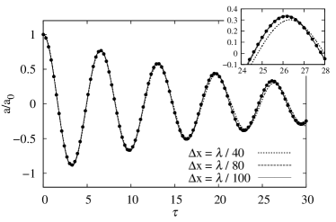
Figure 1: DNS results of the amplitude of a capillary wave of Case A with wavenumber $k=10^{-4}k_{\mathrm{c}}$ as a function of dimensionless time $\tau=t\omega_{0}$ for different mesh spacings $\Delta x$. The analytical solution according to Eq. (12) is shown as solid circles. The inset shows the amplitude for a particular time interval.

Figure 2 shows the dimensionless frequency $\omega/\omega_{\mathrm{m}}$, where $\omega_{\mathrm{m}}$ is the maximum frequency, as a function of dimensionless wavenumber $k/k_{\mathrm{c}}$ obtained with AIVS and DNS. The frequency $\omega$ of the capillary waves is calculated directly from the transient evolution of the amplitude, see for instance Fig. 1, as $\omega=\pi/t_{1}$, where $t_{1}$ is the time of the first extrema of the wave amplitude (e.g. the minima of $a$ in Fig. 1 at $\tau\approx\pi$). The comparison shown in Fig. 2 suggests that the DNS results are accurate for $k\leq 0.9\,k_{\mathrm{c}}$. For $k>0.9\,k_{\mathrm{c}}$ the magnitude of the amplitude at $t_{1}$ becomes $a\sim 10^{-6}\lambda$, which is comparable to the residuals of the numerical solution procedure as well as the model and discretization errors of the DNS methodology. It can therefore be concluded that the DNS is in very good agreement with the AIVS and is a suitable tool to study capillary waves with $k\leq 0.9\,k_{\mathrm{c}}$.

Figure 2: Comparison of the dimensionless frequency $\omega/\omega_{\mathrm{m}}$ as a function of the dimensionless wavenumber $k/k_{\mathrm{c}}$ obtained with AIVS and DNS for Case A. The inset shows the frequency at small wavenumbers and the solid line represents a spline-fit of the AIVS result.

IV Critical damping

As explained in Sec. II, a priori knowledge of the critical wavenumber is important for a consistent characterization of capillary waves. Based on the dispersion relation following from the linearized Navier-Stokes equations, given in Eq. (2), Byrne and Earnshaw (1979) and Hoshino et al. (2008) derived the critical wavenumber as

$$k_{\mathrm{c}}^{\mathrm{B}}=\frac{1.725}{l_{\mathrm{vc}}}\ ,$$ (16)

where superscript $\mathrm{B}$ is reference to the original author(s), since for $k\geq k_{\mathrm{c}}^{\mathrm{B}}$ the roots of Eq. (2) are purely imaginary. This was confirmed experimentally for capillary waves on water-air and glycerol-air interfaces (Byrne and Earnshaw, 1979). A similar critical wavenumber $k_{\mathrm{c}}^{\mathrm{K}}=1.7214\,l_{\mathrm{vc}}^{-1}$ has been proposed by Katyl and Ingard (1968) based on light scattering experiments. In what follows, a new definition of the critical wavenumber is derived based on a harmonic oscillator model, which is shown to be in excellent agreement with AIVS and DNS results.

IV.1 Harmonic oscillator model

Assuming the surface tension coefficient and the viscosity are constant, the oscillation of a capillary wave with small amplitude is described as a harmonic oscillator. For a mass oscillating harmonically in a viscous fluid, the displacement $s$ is given by the second-order ordinary differential equation (Landau and Lifshitz, 1969)

$$\ddot{s}+2\,\zeta\,\omega_{0}\,\dot{s}+\omega_{0}^{2}\,s=0\ .$$ (17)

The undamped frequency $\omega_{0}=\sqrt{c/m}$ is a function of the spring constant $c$ and the mass $m$ of the oscillator, while the damping ratio is

$$\zeta=\frac{b}{2\sqrt{mc}}\ ,$$ (18)

with $b$ being the viscous damping coefficient. With respect to capillary waves, the spring constant is $c=\sigma$ and the mass is $m=\tilde{\rho}/k^{3}$, so that $\omega_{0}=\sqrt{c/m}=\sqrt{\sigma k^{3}/\tilde{\rho}}$, see Eq. (1). Following a dimensional analysis, the viscous damping coefficient can be defined as $b=\tilde{\mu}L$, where $L$ is the damping length.

Based on the lengthscale $l_{\nu}=\sqrt{2\nu/\omega_{0}}$ for the penetration depth of the vorticity generated by a capillary wave (Landau and Lifshitz, 1966; Jenkins and Jacobs, 1997), the critical damping length is defined as

$$L_{\mathrm{c}}=\sqrt{\frac{2\tilde{\mu}}{\omega_{0,\mathrm{c}}\,\tilde{\rho}}}\ ,$$ (19)

where $\omega_{0,\mathrm{c}}=\sqrt{\sigma k_{\mathrm{c}}^{3}/\tilde{\rho}}$ is the undamped frequency at the critical wavenumber $k_{\mathrm{c}}$. Inserting the critical viscous damping coefficient $b_{\mathrm{c}}=\tilde{\mu}L_{\mathrm{c}}$, the mass at critical damping $m_{\mathrm{c}}=\tilde{\rho}/k_{\mathrm{c}}^{3}$ and the spring constant $c=\sigma$ into Eq. (18), the critical damping ratio becomes

$$\zeta_{\mathrm{c}}=\frac{b_{\mathrm{c}}}{2\sqrt{m_{\mathrm{c}}c}}=\frac{\tilde{\mu}L_{\mathrm{c}}}{2\sqrt{\sigma\tilde{\rho}/k_{\mathrm{c}}^{3}}}=1\ .$$ (20)

From Eq. (20) the critical wavenumber based on the harmonic oscillator model (indicated by superscript h.o.) readily follows as

$$k_{\mathrm{c}}^{\ast,\mathrm{h.o.}}=2^{2/3}\,\frac{\sigma\tilde{\rho}}{\tilde{\mu}^{2}}=\frac{2^{2/3}}{l_{\mathrm{vc}}}\ ,$$ (21)

where superscript $\ast$ marks it as a newly proposed value (this notation is applied consistently throughout the manuscript).

However, the critical wavenumber given by Eq. (21) is only accurate for bulk phases with equal density and viscosity. For two-phase systems where the bulk phases have different properties, the critical wavenumber is expanded by the dimensionless property ratio

$$\beta=\frac{\rho_{\mathrm{a}}\rho_{\mathrm{b}}}{\tilde{\rho}^{2}}\,\frac{\nu_{\mathrm{a}}\nu_{\mathrm{b}}}{\tilde{\nu}^{2}}\ ,$$ (22)

with $\tilde{\nu}=\nu_{\mathrm{a}}+\nu_{\mathrm{b}}$, to become

$$k^{\ast}_{\mathrm{c}}=k_{\mathrm{c}}^{\ast,\mathrm{h.o.}}\,(1.0625-\beta)=\frac{2^{2/3}}{l_{\mathrm{vc}}}\,(1.0625-\beta)\ .$$ (23)

This equation accurately predicts the critical wavenumber for capillary waves in fluids with arbitrary properties, as shown below. The property ratio $\beta$ is bounded by the case of a single fluid with a free surface (i.e. $\nu_{\mathrm{b}}=\rho_{\mathrm{b}}=0$) for which $\beta=0$ and the two-phase case with $\rho_{\mathrm{a}}=\rho_{\mathrm{b}}$ and $\nu_{\mathrm{a}}=\nu_{\mathrm{b}}$ for which $\beta=0.0625$. Note that the density ratio in Eq. (22) is also included in the AIVS as proposed by Prosperetti (1981), see Eqs. (12) and (13), where it is associated with the continuity of tangential stresses at the interface, and appears in the damping rate proposed by Jeng et al. (1998) for small damping.

Comparing the critical wavenumber $k_{\mathrm{c}}^{\ast}$ predicted by the proposed harmonic oscillator model, Eq. (23), with the critical wavenumber $k_{\mathrm{c}}^{\mathrm{B}}$ derived from the linearized Navier-Stokes equations (weak damping assumption), Eq. (16), yields a difference ranging from $2.3\%$ for $\beta=0$ to $8.7\%$ for $\beta=0.0625$. Hence, the difference is largest for two-phase systems in which both bulk phases have equal properties ($\beta=0.0625$) and smallest for a single fluid with a free surface ($\beta=0$).

In practice this means, for instance, that a capillary wave on a water-air interface at room temperature has a critical wavenumber of $k_{\mathrm{c}}^{\ast}=1.17\times 10^{8}\,\mathrm{m}^{-1}$, which corresponds to a critical wavelength of $\lambda_{\mathrm{c}}^{\ast}=5.37\times 10^{-8}\,\mathrm{m}$. This compares to a critical wavenumber of $k_{\mathrm{c}}^{\mathrm{B}}=1.24\times 10^{8}\,\mathrm{m}^{-1}$ ($\lambda_{\mathrm{c}}^{\mathrm{B}}=5.07\times 10^{-8}\,\mathrm{m}$) based on the linearized Navier-Stokes equations, a difference in wavenumber of $6.95\times 10^{6}\,\mathrm{m}^{-1}$, which corresponds to a difference in critical wavelength of $3.03\times 10^{-9}\,\mathrm{m}$. For a capillary wave on an interface between glycerol and air, the critical wavenumber is $k_{\mathrm{c}}^{\ast}=60\,\mathrm{m}^{-1}$, corresponding to a critical wavelength of $\lambda_{\mathrm{c}}^{\ast}=0.11\,\mathrm{m}$, which exemplifies the wide range of critical wavenumbers found in typical engineering applications and natural processes, from the nanoscale to the macroscale.

IV.2 Balance of scales

It is worth recalling, that surface tension and viscous stresses are the dominant physical mechanisms for capillary waves, as discussed in Sec. II. The Ohnesorge number, see Eq. (4), which compares the characteristic timescales of surface tension and viscous stresses, at critical damping with $l=1/k_{\mathrm{c}}^{\ast}$ is

$$\mathrm{Oh}_{\mathrm{c}}=\tilde{\mu}\,\sqrt{\frac{k_{\mathrm{c}}^{\ast}}{\sigma\tilde{\rho}}}=2^{1/3}\,\sqrt{1.0625-\beta}\ .$$ (24)

Rearranging this equation for $k_{\mathrm{c}}^{\ast}$ leads back to Eq. (23). This suggests that at critical damping the dispersive/restoring mechanism (surface tension) and the dissipative mechanism (viscous stresses) reach a specific balance; hence, occur at a specific relative timescale. Since, with lengthscale $l=1/k_{\mathrm{c}}^{\ast}$, the capillary timescale is the inverse of the frequency of a capillary wave with wavenumber $k_{\mathrm{c}}^{\ast}$ in inviscid fluids, $t_{\sigma}=\omega_{0,\mathrm{c}}^{-1}=\sqrt{\sigma k_{\mathrm{c}}^{\ast}/\tilde{\rho}}$, the balance of capillary and viscous effects described by Eq. (24) means that the viscous timescale at critical damping is $t_{\mu}\sim\beta^{-1/2}\,\omega_{0,\mathrm{c}}^{-1}$. This suggests that the viscous attenuation of capillary waves is only dependent on the frequency $\omega_{0}$ (and, consequently, the phase velocity $c_{0}=\omega_{0}/k$) and on the fluid property ratio $\beta$.

IV.3 Validation

Figure 3 shows the dimensionless undamped frequency $\omega_{0}/\omega_{0,\mathrm{c}}$ as a function of the dimensionless wavenumbers $k/k_{\mathrm{c}}^{\ast}$, proposed in Eq. (23), and $k/k_{\mathrm{c}}^{\mathrm{B}}$, given by Eq. (16), with $\omega_{0,\mathrm{c}}$ being the undamped frequency at $k_{\mathrm{c}}$. The dimensionless frequencies for the displayed cases fall on a single line when the proposed critical wavenumber $k^{\ast}_{\mathrm{c}}$ is used as a basis for the normalization, suggesting that $k_{\mathrm{c}}^{\ast}$ is a characteristic value of the frequency dispersion of capillary waves. In contrast, no consistent correlation between $\omega_{0}/\omega_{0,\mathrm{c}}$ and $k/k_{\mathrm{c}}^{\mathrm{B}}$ is observed, see Fig. 3b. This supports the findings of Jeng et al. (1998), who reported that weak damping is not an adequate assumption for the entire underdamped regime, since $k_{\mathrm{c}}^{\mathrm{B}}$ is derived from the dispersion relation given in Eq. (2) and is, therefore, based on the weak damping assumption.

(a) Scaled based on $k_{\mathrm{c}}^{\ast}$

(b) Scaled based on $k_{\mathrm{c}}^{\mathrm{B}}$

Figure 3: Dimensionless undamped frequency $\hat{\omega}_{0}=\omega_{0}/\omega_{0,\mathrm{c}}$ as a function of dimensionless wavenumber $k/k_{\mathrm{c}}^{\ast}$, based on the proposed critical wavenumber given in Eq. (23), and $k/k_{\mathrm{c}}^{\mathrm{B}}$, based on the critical wavenumber given in Eq. (16).

Figure 4 shows the damping ratio $\zeta$ as a function of the dimensionless wavenumber $\hat{k}=k/k_{\mathrm{c}}^{\ast}$ for the cases considered with AIVS. Despite the large variety of fluid properties of these cases (i.e. spanning the entire possible $\beta$-range), the solutions consistently approach and cross $\zeta=1$ at critical damping ($\hat{k}=1$) within the expected margins of error. Note that for $\hat{k}=1$ the AIVS still shows oscillatory behavior of the wave amplitude. However, the wave amplitude at the first extrema has a magnitude of $|a_{1}|\approx 10^{-14}$. This error can be attributed to the finite precision of floating point arithmetic, which is approximately $2.22\times 10^{-16}$ on a 64-bit system according to IEEE Standard 754, in conjunction with the large number of conducted time-steps (e.g. $6996$ time-steps to $t_{1}$ for Case A). Moreover, the waves exhibit no oscillations for $\hat{k}=1.01$.

Figure 4: Damping ratio $\zeta$ as a function of dimensionless wavenumber $\hat{k}=k/k_{\mathrm{c}}^{\ast}$ for the considered cases obtained with AIVS, where point $(1,1)$ represents critical damping. Note that $\zeta\geq 1$ for $\hat{k}<1$ and $\zeta\leq 1$ for $\hat{k}>1$ are not part of the physical parameter space.

V Dispersion similarity

Having the means to accurately predict the critical wavenumber, and considering that a universal formulation of the critical wavenumber is possible, raises the question if the dispersion of capillary waves is in fact self-similar following an appropriate scaling.

Figure 5a shows the dimensionless frequency $\hat{\omega}=\omega\,t_{\mathrm{vc}}$ as a function of dimensionless wavenumber $\hat{k}=k/k_{\mathrm{c}}^{\ast}$ obtained with AIVS for Cases A-D. The results fall on a single line in the $\hat{k}-\hat{\omega}$ graph throughout the entire underdamped regime, with a single dimensionless frequency $\hat{\omega}$ for every dimensionless wavenumber $\hat{k}$. The same similarity is exhibited by the DNS results of Cases A, E and F, shown in Fig. 5b. Thus, normalizing the frequency based on the viscocapillary timescale $t_{\mathrm{vc}}$, see Eq. (7), and normalizing the wavenumber with the proposed critical wavenumber $k_{\mathrm{c}}^{\ast}$, see Eq. (23), leads to a self-similar characterization of the frequency dispersion of capillary waves. Since a specific dimensionless frequency $\hat{\omega}$ can be associated with each dimensionless wavenumber $\hat{k}$, the frequency for capillary waves of any wavenumber is readily available based on the solution for one particular two-phase system, for instance obtained with AIVS or from experiments, and irrespective of the fluid properties. This similarity also provides further evidence for the balance of capillary and viscous timescales and the ensuing dependency of the viscous attenuation on fluid properties and wavenumber only, as proposed in Sec. IV.2.

(a) AIVS results

(b) DNS results

Figure 5: Dimensionless frequency $\hat{\omega}=\omega\,t_{\mathrm{vc}}$ as a function of dimensionless wavenumber $\hat{k}=k/k_{\mathrm{c}}^{\ast}$ obtained with AIVS and DNS. The inset shows the frequency of capillary waves with small wavenumbers.

Based on the presented AIVS and DNS results the maximum frequency is

$$\omega_{\mathrm{m}}^{\ast}=\frac{0.488}{t_{\mathrm{vc}}}\ ,$$ (25)

which accurately quantifies the maximum frequency in all considered cases. Furthermore, the maximum frequency is consistently observed in the presented results at approximately

$$k^{\ast}_{\mathrm{m}}=0.751\,k_{\mathrm{c}}^{\ast}\ .$$ (26)

Note that the correction using the property ratio $\beta$ included in $k_{\mathrm{c}}^{\ast}$, see Eq. (23), also applies to $k^{\ast}_{\mathrm{m}}$. Thus, the maximum frequency is a characteristic value of the dispersion of capillary waves, as discussed in Sec. II. Ingard (1988) proposed empirical estimates for the maximum frequency $\omega_{\mathrm{m}}^{\mathrm{I}}=0.46244\,t_{\mathrm{vc}}^{-1}$ and the corresponding wavenumber $k_{\mathrm{m}}^{\mathrm{I}}=1.2797\,l_{\mathrm{vc}}^{-1}$, which however result in a smaller maximum frequency and larger corresponding wavenumber than observed in the results presented in Fig. 5.

The maximum frequency of a capillary wave on a water-air interface is $\omega_{\mathrm{m}}^{\ast}=2.52\times 10^{9}\,\mathrm{s}^{-1}$ at $k_{\mathrm{m}}^{\ast}=8.79\times 10^{7}\,\mathrm{m}^{-1}$ ($\lambda_{\mathrm{m}}^{\ast}=7.15\times 10^{-8}\,\mathrm{m}$), whereas for a capillary wave on an interface between glycerol and air, the maximum frequency of $\omega_{\mathrm{m}}^{\ast}=0.9\,\mathrm{s}^{-1}$ occurs at $k_{\mathrm{m}}^{\ast}=45.1\,\mathrm{m}^{-1}$ ($\lambda_{\mathrm{m}}^{\ast}=0.14\,\mathrm{m}$). The range of maximum frequencies for practically relevant two-phase systems, hence, spans over several orders of magnitude, similar to the range of practically relevant critical wavenumbers discussed in Sec. IV.1. The maximum frequency for an water-air system ($\omega_{\mathrm{m}}\approx 10^{9}\,\mathrm{s}^{-1}$) is several orders of magnitude larger than the typical maximum frequencies ($\omega\lesssim 10^{3}-10^{4}\,\mathrm{s}^{-1}$) with appreciable energy (Deike et al., 2012, 2014a; Abdurakhimov et al., 2015) of freely decaying capillary wave turbulence and should, thus, not be a limiting factor for practical applications or experimental studies of capillary wave turbulence.

VI Damping regimes and assumptions

As mentioned in the introduction, the damping provided by viscous stresses in the underdamped regime is not accurately described by commonly used assumptions. Figure 6 shows the dimensionless damping rate $\hat{\Gamma}=\Gamma\tilde{\rho}/(\tilde{\mu}k^{2})$ as a function of dimensionless wavenumber $\xi=k/k^{\ast,\mathrm{h.o.}}_{\mathrm{c}}$, which is based on the critical wavenumber obtained from the proposed harmonic oscillator model $k^{\ast,\mathrm{h.o.}}_{\mathrm{c}}$, see Eq. (21), without the expansion using the property ratio $\beta$. The dimensionless damping rate $\hat{\Gamma}$ changes considerably for different $\xi$, and at small wavenumbers $\hat{\Gamma}$ is also dependent on the fluid properties. A similar observation can be made in Fig. 4, since the damping ratio $\zeta$ develops differently as a function of $\hat{k}$ for each of the considered two-phase systems and, thus, the capillary waves experience a different effective damping rate $\Gamma=\zeta\omega_{0}$ in each two-phase system.

Figure 6: Dimensionless damping rate $\hat{\Gamma}=\Gamma\tilde{\rho}/(\tilde{\mu}k^{2})$ as a function of dimensionless wavenumber $\xi=k/k_{\mathrm{c}}^{\ast,\mathrm{h.o.}}$ obtained with AIVS for Cases A ($\beta=0.0625$) and D ($\beta=0$) and with DNS for Case E ($\beta=7\times 10^{-5}$). The inset shows the dimensionless damping rate at small wavenumbers.

For $\xi\gtrsim 0.1$, the results shown in Fig. 6 suggest a similarity of $\hat{\Gamma}$, since all results fall on a single line, thus delineating a distinct regime of the dispersion of capillary waves. In this regime of significant damping the dimensionless damping rate is well approximated by the correlation

$$\hat{\Gamma}=0.6868\,\xi^{-1/4}+0.1\,\xi^{-1/2}\ ,$$ (27)

as seen in Fig. 6. Hence, the frequency in this regime can be readily estimated as

$$\bar{\omega}^{\ast}=\omega_{0}+i\frac{\tilde{\mu}k^{2}}{\tilde{\rho}}\,(0.6868\,\xi^{-1/4}+0.1\,\xi^{-1/2})\ .$$ (28)

In order to show the differences between frequency estimates based on different assumptions, Fig. 7 shows the relative error

$$\varepsilon(\hat{k})=\frac{|\bar{\omega}(\hat{k})-\omega(\hat{k})|}{{\omega}(\hat{k})}\ .$$ (29)

of $\bar{\omega}^{\ast}$ alongside frequency estimates given by the undamped frequency

$$\bar{\omega}^{\mathrm{(i)}}=\omega_{0}\ ,$$ (30)

with $\omega_{0}$ defined in Eq. (1), and based on the weak damping assumption

$$\bar{\omega}^{\mathrm{(ii)}}=\omega_{0}+i\Gamma_{0}\ ,$$ (31)

with $\Gamma_{0}=2\tilde{\mu}k^{2}/\tilde{\rho}$ (Jeng et al., 1998). The frequency estimate proposed in Eq. (28) exhibits a high accuracy throughout the underdamped regime, as seen in Fig. 7a. Due to the definition of the relative error given in Eq. (29), $\varepsilon$ increases rapidly as $\hat{k}\rightarrow 1$ since $\omega\rightarrow 0$. At small wavenumbers (long wavelength) the frequency of capillary waves in viscous fluids is well approximated by neglecting the influence of viscous stresses using the frequency estimate $\bar{\omega}^{\mathrm{(i)}}$, as seen in Fig. 7b, with $\varepsilon<6\%$ for $\hat{k}\leq 10^{-3}$, and a rapidly reducing error for decreasing wavenumbers. The frequency estimate $\bar{\omega}^{\mathrm{(ii)}}$ based on the weak damping assumption provides a good estimate up to $\hat{k}\approx 0.07$, with $\varepsilon<8\%$, as observed in Fig. 7c.

(a) Error $\varepsilon$ based on $\bar{\omega}^{\ast}$

(b) Error $\varepsilon$ based on $\bar{\omega}^{\mathrm{(i)}}$

(c) Error $\varepsilon$ based on $\bar{\omega}^{\mathrm{(ii)}}$

Figure 7: Relative error $\varepsilon$, see Eq. (29), of the frequency predictions given in Eqs. (28), (30) and (31) with respect to the frequencies obtained from AIVS and DNS as a function of dimensionless wavenumber $\hat{k}$.

Note that the error of $\bar{\omega}^{\mathrm{(i)}}$ and $\bar{\omega}^{\mathrm{(ii)}}$ is substantially smaller for Cases D and E, i.e. for two-phase systems with very different fluid properties of the bulk phases ($\beta\rightarrow 0$), than for Case A ($\beta=0.0625$). This is presumably the reason why linear wave theory based on inviscid fluids or the weak damping assumption is frequently found to be in very good agreement with experiments and numerical simulations that have so far mostly focused on gas-liquid systems (e.g. water-air systems), for which $\beta\approx 0$. For example, Byrne and Earnshaw (1979) reported the critical wavenumber $k_{\mathrm{c}}^{\mathrm{B}}$, given in Eq. (16), which is derived from the weak damping assumption, to be in good agreement with their experimental measurements at water-air and glycerol-air interfaces. However, the results of Case A ($\beta=0.0625$) suggest that for two-phase systems with bulk phases of similar fluid properties, such as immiscible liquid-liquid flows, the frequency error ensuing from the weak damping assumption is large enough to have a practical impact and to be measured experimentally.

The results presented in Fig. 6 suggest that, assuming the same cumulative properties $\tilde{\rho}$, $\tilde{\mu}$ and $\tilde{\nu}$ of the two-phase system, systems with high ratios of kinematic viscosity or density ($\beta\rightarrow 0$) impose a smaller effective viscous damping than two-phase systems in which the ratios of kinematic viscosity and density are unity ($\beta=0.0625$). Hence, two-phase systems with $\beta\rightarrow 0$, e.g. Case D, require a higher wavenumber to oscillate with a certain dimensionless frequency $\hat{\omega}$ or to exhibit critical damping. This explains the observed shift to higher wavenumbers in Eq. (23) for critical damping for two-phase systems with smaller $\beta$.

VII Conclusions

In order to characterize the frequency dispersion of capillary waves in viscous fluids, a rational parametrization based on a harmonic oscillator model has been proposed, from which a formulation for the critical wavenumber has been derived. This critical wavenumber has been shown to be a characteristic value of the frequency dispersion of capillary waves, as demonstrated by the consistent scaling of the undamped frequency $\omega_{0}$ as well as the damping rate computed with AIVS and DNS for representative two-phase systems. Critical damping occurs when capillary and viscous timescales are in balance, a finding which may also apply to other damped oscillators, such as elastic membranes, in that critical damping occurs when suitably defined dispersive (or restoring) and dissipative timescales are in balance.

The proposed scaling of capillary waves together with the critical wavenumber obtained from the proposed harmonic oscillator model has been shown to lead to a self-similar characterization of the frequency dispersion of capillary waves, irrespective of the fluid properties and throughout the entire underdamped regime. The identified similarity of the frequency dispersion allows to take, for instance, experimental measurements or results obtained with the AIVS of Prosperetti (1981) for certain fluid properties and translating these results to any other two-phase system using the proposed scaling. Since analytical solutions for simple reference cases are readily available, this similarity, thus, enables an accurate a priori evaluation of the frequency of a capillary wave in viscous fluids for any wavenumber. Also, this similarity yields the conclusion that the wavenumber is a function of the viscocapillary lengthscale and the property ratio, $k\sim l_{\mathrm{vc}}^{-1}(1.0625-\beta)$, and the frequency is a function of the viscocapillary timescale, $\omega\sim t_{\mathrm{vc}}^{-1}$. Being able to accurately predict the dispersion of capillary waves for arbitrary wavenumbers, can for instance help to better understand the characteristics (e.g. wavelength) of parasitic capillary waves riding on gravity waves or the influence of viscous stresses on the capillary-driven breakup of liquid jets, processes which are governed by nonlinear interactions between various governing mechanisms.

The inviscid and weak damping assumptions, which are commonly used to describe the dispersion of capillary waves, have been shown to be inaccurate for high wavenumbers, close but below the critical wavenumber. With respect to the assumption of inviscid fluids, the presented results suggest this to be valid for wavenumbers $\hat{k}\lesssim 10^{-3}$. Interestingly, the weak damping assumption provides a considerably more accurate description of two-phase systems in which the bulk phases have large density and viscosity ratios than for systems with similar bulk phases. A new definition of the damping rate based on the AIVS and DNS results has been proposed, which has been shown to yield a more accurate prediction of the frequency of capillary waves at high wavenumbers than estimates based on the inviscid and weak damping assumptions.