Effects of contact-line pinning on the adsorption of nonspherical colloids at liquid interfaces

Abstract

The effects of contact-line pinning are well-known in macroscopic systems, but are only just beginning to be explored at the microscale in colloidal suspensions. We use digital holography to capture the fast three-dimensional dynamics of micrometer-sized ellipsoids breaching an oil-water interface. We find that the particle angle varies approximately linearly with the height, in contrast to results from simulations based on minimization of the interfacial energy. Using a simple model of the motion of the contact line, we show that the observed coupling between translational and rotational degrees of freedom is likely due to contact-line pinning. We conclude that the dynamics of colloidal particles adsorbing to a liquid interface are not determined by minimization of interfacial energy and viscous dissipation alone; contact-line pinning dictates both the timescale and pathway to equilibrium.

The adsorption of a microscopic colloidal particle to a liquid interface is a dynamic wetting process: in the reference frame of the particle, the three-phase contact line moves along the particle’s surface. Our understanding of analogous wetting processes in macroscopic systems is based on two types of models: those that relate the motion of the contact line to the viscous dissipation in the fluid “wedge” bounded by the solid and the liquid interface Huh and Scriven (1971); Dussan V. and Davis (1974); de Gennes (1985), and those that consider dissipation local to the contact line Blake and Haynes (1969); Blake (2006). Models in this second class treat the motion of the contact line as a thermally activated process, in which the contact line transiently pins on nanoscale defects and hops between them. The two viewpoints are not incompatible: both types of dissipation can be relevant to experiments Brochard-Wyart and de Gennes (1992), and thermally activated motion of the contact line can be viewed as a model for how slip occurs at the solid boundary Snoeijer and Andreotti (2013). The nanoscale defects responsible for pinning the contact line are now understood to be important in macroscopic wetting experiments at small capillary number Prevost et al. (1999); Rolley and Guthmann (2007); Snoeijer and Andreotti (2013) and in phenomena related to contact-angle hysteresis Giacomello et al. (2016).

Figure 1: a) Schematic showing the cross-section through the long axis of an ellipsoidal particle breaching an interface. Simulations assuming interfacial energy is minimized at each time step predict trajectories (solid lines) that are non-monotonic in both center-of-mass position and polar angle Günther et al. (2014); de Graaf et al. (2010). Our experimental results (shaded ellipses) show a monotonic increase in both height and polar angle. See also the movie in the Supplemental Material Not . b) Schematic of contact-line motion for one scenario in a). A line shows where the contact line moves in the frame of reference of the particle after time $\Delta$t. The dynamic contact angles at two points are shown.

Such defects—and the associated hopping of the contact line—have also proven important for understanding the dynamics of microscopic colloidal particles at liquid interfaces. These particles can strongly adhere to the interface, owing to the large change in the total interfacial energy of the system once the particles bind Binks (2007). The resulting systems are used to study phase transitions and self-assembly in two dimensions Pieranski (1980); Aveyard et al. (2000); Zahn and Maret (2000); Bausch et al. (2003); König et al. (2005); Cavallaro et al. (2011); Botto et al. (2012), to fabricate new materials Paunov and Cayre (2004); Retsch et al. (2009); Isa et al. (2010), and to formulate Pickering emulsions and colloidosomes Ramsden (1903); Pickering (1907); Dinsmore et al. (2002); McGorty et al. (2010). But nearly all particles used in such systems have nanoscale surface features that can pin the contact line Wang et al. (2016). Whereas strong pinning sites can affect interactions Kralchevsky et al. (2001) and motion on curved interfaces Sharifi-Mood et al. (2015), even weak pinning sites can dramatically affect dynamics. For example, Boniello and coworkers Boniello et al. (2015) showed that the in-plane diffusion of particles straddling an air-water interface is inconsistent with models of viscous drag in the bulk fluids but consistent with models of contact-line fluctuations caused by nanoscale defects. Also, Kaz, McGorty, and coworkers Kaz et al. (2012) showed that spherical colloidal particles breaching liquid interfaces relax towards equilibrium at a rate orders of magnitude slower than that predicted by models of viscous dissipation in a fluid wedge. Dynamic wetting models based on thermally activated hopping Blake and Haynes (1969); Colosqui et al. (2013) fit the observed adsorption trajectories well over a wide range of timescales.

Here we examine the effects of transient pinning and depinning on the pathway that ellipsoidal colloidal particles take to equilibrium, and not just the time required to get there. By “pathway” we mean the way in which the degrees of freedom vary with time. For example, a spherical particle has one degree of freedom—its height relative to the interface. Its pathway to equilibrium does not depend on pinning effects: at low Reynolds number, the height changes monotonically with time, regardless of whether the contact line becomes pinned along the way. By contrast, an ellipsoid of revolution, or spheroid, has two degrees of freedom—its center-of-mass position and orientation—which need not vary monotonically with time. In fact, molecular dynamics Günther et al. (2014) and Langevin dynamics studies de Graaf et al. (2010) predict that both the height and orientation of ellipsoidal particles breaching an interface vary non-monotonically with time (Figure 1a). These simulations assume that the particles follow a quasi-static approach to equilibrium, such that the total interfacial energy is minimized at each step along the way, and they do not model contact-line pinning. They predict an equilibration time of 10 $\mu$s based on the viscous dissipation, but previous experimental studies of prolate spheroids at interfaces by Coertjens et al. Coertjens et al. (2014) and Mihiretie et al. Mihiretie (2013) suggest that the equilibration time is much longer, hinting at pinning effects.

We use a fast 3D imaging technique, digital holographic microscopy, to observe ellipsoidal (prolate spheroidal) colloidal particles adsorbing to an oil-water interface. We find that not only is the equilibration time orders of magnitude larger than that predicted by simulations, but the position and orientation of the particle vary monotonically with time, in contrast to the nonmonotonic pathways found in simulations de Graaf et al. (2010); Günther et al. (2014). Interestingly, the center-of-mass position and the polar angle of the particle are coupled, so that the particle “rolls” into its equilibrium position as if it were subject to a tangential frictional force (Figure 1a and Supplemental Material Not ). We argue that these effects are due to contact-line pinning.

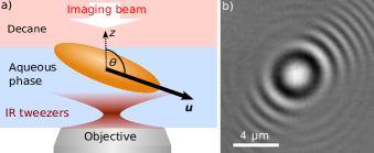
Figure 2: Schematic of experimental setup. a) The sample is illuminated with a red collimated laser ($\lambda$ = 660 nm). A counterpropagating infrared laser ($\lambda$ = 785 nm) is used to gently push the particles against gravity towards the interface. In the coordinate system used here, the imaging axis lies along $z$, and the interface is at $z$=0. The center-of-mass position and the polar angle $\theta$ of the particle are defined relative to the laboratory frame by a unit vector $\mathbf{u}$ that points along the long axis of the ellipsoid. b) A typical hologram of an ellipsoid at an interface. See also the movie in the Supplemental Material Not .

To make ellipsoidal particles, we heat 1.0-$\mu$m-diameter sulfate-functionalized polystyrene particles (Invitrogen) above their glass transition temperature and stretch them Not . Using the apparatus shown in Figure 2, we capture holograms of individual ellipsoids at 100 frames per second as they approach an interface between decane and a water/glycerol mixture. The holograms encode the three-dimensional position and orientation of the particle in the spacing and shape of the interference fringes. We extract this information, along with the particle size and refractive index, by fitting a T-matrix model Mishchenko and Travis (1998) of the scattering from the particles to our data Not .

We find that the particles relax to equilibrium slowly, despite some abrupt motion along the way, as shown in Figure 3a. After 1 s, or five orders of magnitude longer than the equilibrium time observed in simulations de Graaf et al. (2010), the particles are still not equilibrated. Furthermore, their height scales roughly linearly with the logarithm of the elapsed time after the breach. Because this is the same scaling observed by Kaz and coworkers Kaz et al. (2012), the likely origin of the slow dynamics is contact-line pinning and depinning, the same mechanism observed in spherical particles. The slow dynamics are perhaps unsurprising, since the particles are stretched versions of those used by Kaz et al. Kaz et al. (2012).

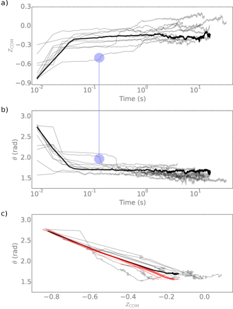
Figure 3: The height (a) and polar angle $\theta$ (b) of ellipsoids after they breach (breach at $t$ = 0 s) appear correlated (example marked with blue circles). To compare data from particles of different aspect ratios on the same plot, we normalize the center-of-mass height relative to the interface de Graaf et al. (2010) to obtain $z_{\mathrm{COM}}=z/\sqrt{2a^{2}+b^{2}}$ , where $a$ and $b$ are the semi-minor and semi-major axes of the spheroid. c) The polar angle varies with the height. Our model (red), based on contact-line hopping over defects, produces almost linear relationships between $z$ and $\theta$ for the particles from the experiments.

More surprisingly, we find that the abrupt changes in height (Figure 3a) correlate with abrupt changes in the polar angle $\theta$ (Figure 3b). Indeed, when we examine $\theta$ as a function of $z$ we find that the relationship is approximately linear (Figure 3c). Furthermore, although the particles approach the interface from a variety of different polar angles, the $\theta$–$z$ plots form lines with similar slopes, hinting at the presence of a dynamical attractor.

The linear relationship between $\theta$ and $z$ is reminiscent of rolling, where translation and rotation are coupled by friction. The particles “pivot” into the interface, as shown by the rendering of individual points along the observed trajectories (Figure 1a and Supplemental Material Not ). In contrast, the simulations by Günther et al. Günther et al. (2014) and de Graaf et al. de Graaf et al. (2010) predict that $\theta$ and $z$ should vary non-monotonically in time (Figure 1a).

We therefore seek a different model to explain the observed rotational-translational coupling, one that takes into account contact-line pinning. We adopt the viewpoint of Kaz et al. Kaz et al. (2012) and assume that the contact line pins to defects on the surface of the particle and hops between pinning sites with the aid of thermal kicks. We calculate the velocity of the contact line using an Arrhenius equation coupled to a model for the force, determined by the dynamic contact angle $\alpha_{\mathrm{D}}(t)$. In contrast to the model for spheres, our model allows $\alpha_{\mathrm{D}}(t)$ to vary as a function of position on the particle, though we still assume that the interface remains flat at all times, a simplification that we justify based on the energetic cost of bending the interface.

For a horizontal interface defined by a denser aqueous phase on the bottom and an oil phase on top (Figure 2), the force on each segment of the contact line is then determined from the imbalance between the three interfacial tensions (oil–water $\sigma_{\mathrm{ow}}$, particle–water $\sigma_{\mathrm{pw}}$, and particle–oil $\sigma_{\mathrm{po}}$):

$$\begin{split}F_{\mathrm{cl}}&={\sigma}_{\mathrm{ow}}\cos{\alpha}_{\mathrm{D}}(t)+\sigma_{\mathrm{pw}}-\sigma_{\mathrm{po}}\\ &={\sigma}_{\mathrm{ow}}\left(\cos{\alpha}_{\mathrm{D}}(t)-\cos{\alpha}_{\mathrm{E}}\right)\end{split}$$ (1)

where $\alpha_{\mathrm{E}}$ is the equilibrium contact angle. To understand this relation, consider Figure 1b. The force is tangent to the particle. Because the contact angle is defined relative to the aqueous phase, $F_{\mathrm{cl}}$ is positive and the contact line moves down the particle (in the particle frame) if the particle approaches the interface from the aqueous phase (${\alpha}_{\mathrm{D}}<{\alpha}_{\mathrm{E}}$). If the particle approaches the interface from the oil phase (${\alpha}_{\mathrm{D}}>{\alpha}_{\mathrm{E}}$), $F_{\mathrm{cl}}$ is negative and the contact line moves up the particle. Because the particle is nonspherical, the force per unit length along the contact line is asymmetric about the short axis of the ellipsoid unless the particle breaches the interface at exactly $\theta$ = $\pi$/2.

The direction and magnitude of this force determine the velocity of the contact line along the particle surface. We relate $F_{\mathrm{cl}}$ to the velocity of the contact line using an Arrhenius equation that is valid when forward hops dominate Blake and Haynes (1969); Kaz et al. (2012) ($\lvert\alpha_{\mathrm{E}}-\alpha_{\mathrm{D}}\rvert\gtrsim 0.01$, as discussed in the Supplemental Material Not ):

$$V=\frac{F_{\mathrm{cl}}(t)}{\lvert F_{\mathrm{cl}}(t)\rvert}V_{0}\exp\left(-\frac{U}{kT}+\frac{\lvert F_{\mathrm{cl}}(t)\rvert A}{2kT}\right)$$ (2)

where $V$ is the velocity of the contact line tangent to the particle, $V_{0}$ is a molecular velocity scale, $A$ is the area per defect on the surface of the particle, and $U$ is the energy with which each defect pins the contact line. When spherical particles start in the aqueous phase, Equation 2 reduces to the form described in the Supplementary Information of Kaz et al. Kaz et al. (2012). Further details of the model are given in the Supplemental Material Not .

Before comparing the model to the data, we first determine which parameters in the model control the trajectory. The dynamic contact angle is greater near the tips of the particle than it is near the center ($\alpha_{\mathrm{D,tip}}>\alpha_{\mathrm{D,center}}$), as illustrated in Figure 1b. The part of the contact line nearest the tip travels more slowly than the part nearest the center ($V_{\mathrm{tip}}<V_{\mathrm{center}}$ according to Equations 1 and 2), leading to the observed pivoting motion. Considering only these two points, the ratio $V_{\mathrm{center}}$/$V_{\mathrm{tip}}$ = $\exp\left(\sigma_{\mathrm{ow}}A\left(\cos\alpha_{\mathrm{D,center}}-\cos\alpha_{\mathrm{D,tip}}\right)/2kT\right)$ approximates the rate at which $z$ and $\theta$ change relative to each other. We therefore expect the shape and aspect ratio of the particle, which determine the values of $\alpha_{\mathrm{D}}$ for a given $\theta$ and $z$, and the area per defect $A$ to control the form of the $\theta$–$z$ curve. Changing the size of the particle, $U$, or $\alpha_{\mathrm{E}}$ alters how $\theta$ and $z$ depend on time, but not how $\theta$ and $z$ evolve with each other. We explore the effect of particle shape further below.

The model produces trajectories that agree with experimental observations. In Figure 3c, we plot calculated $\theta$-$z$ trajectories for each of the particles using the measured aspect ratio determined from fitting the holograms and a defect area equal to that measured in Kaz et al. Kaz et al. (2012), $A$ = 4 nm². We have strong evidence that $A$ is nanoscale, as discussed in the Supplemental Material Not . The modeled $\theta$ and $z$ are both monotonic with time, in contrast to the predictions from earlier simulations. Moreover, $\theta$ varies linearly with $z$, reproducing the translational-rotational coupling in our experimental results. The slope predicted by the model (-1.75 $\pm$ 0.16 rad) agrees with the average slope in our experimental results (-1.64 $\pm$ 0.76 rad).

Our model predicts that all trajectories collapse onto one line for a given $A$ (Figure 3c). de Graaf and coworkers found a similar “dynamical attractor” for ellipsoids in their Langevin simulations de Graaf et al. (2010), while Günther et al. Günther et al. (2014) found that the adsorption trajectory depends sensitively on the angle of the particle when it first touches the interface. Our model predicts an attractor, but the attractor arises from the pinning, and in particular from how pinning ensures that the contact-line velocity near the tip is always smaller than that near the center.

The only discrepancy between the model and our data is that the slopes of the modeled trajectories are more narrowly distributed than the experimentally observed slopes. This discrepancy may be due to deviations in shape from perfect prolate spheroids (see image of the particles in the Supplementary Material Not ), which would affect the curvature of the particle and hence $\alpha_{\mathrm{D}}$. The area per defect $A$ might also vary between particles. Our data falls between the calculated attractors for particles with $A$ = 1 nm² and 30 nm². Finally, the stretching of the particles might lead to an inhomogeneous defect density, which we do not account for in our model. However, the agreement between the average observed and calculated slopes suggest that our assumption of a uniform defect density is valid to within the uncertainties of our measurements Not .

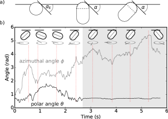
Figure 4: a) A hydrophilic spherocylinder ($\alpha_{\mathrm{E}}<$ $\pi$/4; hemispherical caps drawn in dotted lines) can reach a local minimum in the interfacial energy when the contact angle $\alpha$ = $\alpha_{\mathrm{E}}$. b) Experimental data showing that a hydrophilic silica spherocylinder freely rotates about the $z$-axis once it has attached to the interface (shaded region), but its polar angle remains fixed. Arrows indicate the particle’s polar and azimuthal angles at the time points indicated by the red dotted lines.

Our model further predicts that if the particles were spherical, there would be no net torque on the particle, owing to the symmetry. To verify this prediction, we examine spherocylindrical particles (Figure 4), each of which consists of a cylinder with hemispherical caps. If the spherocylinder is hydrophilic, such that a sphere of the same material has an equilibrium contact angle smaller than $\pi/4$ (Figure 4a), it can attach to the interface at a range of polar angles all having the same energy (Figure 4a). Our model predicts that the contact line will not exert a torque on the particle and that the particle should therefore remain at the same polar angle.

Indeed, we observe that when hydrophilic spherocylinders breach the interface, their polar angle remains fixed, although their azimuthal angle can still fluctuate (Figure 4b). The absence of equilibration is surprising because the minimum-energy configuration for spherocylinders is $\theta$ = $\pi/2$. However, the observed trajectories agree with the prediction of our model.

We therefore conclude that accounting for contact-line pinning, and not just interfacial energy, is necessary to understand the dynamics of nonspherical particles at liquid interfaces. The slow relaxation observed in such systems is just one manifestation of the pinning; as we have shown here, the pinning can also alter the pathway to equilibrium. The agreement between model and experiment suggests that the pathway is controlled not only by the size of the defects on the solid surfaces, but also by the local curvature of the particle. Thus, not only is the road to equilibrium long, but it also depends on the details of the shape of the particle.

These results have practical implications for assembling particles at an interface and, at the same time, lead to new fundamental understanding of how dynamic wetting influences particles at interfaces. In terms of practical implications, the unexpectedly long adsorption times we find in our experiments might significantly affect the aging of Pickering emulsions. Although we have neglected the curvature of the interface in our simple dynamical model, ellipsoidal particles should induce a quadrupolar capillary field in equilibrium Loudet et al. (2005). Therefore the equilibration of multiple particles at the interface might be complicated by the slowly evolving capillary interactions between them. Also, the shape of the particle might play a large role in determining if and how such systems arrive at equilibrium. Particles like the spherocylinder (and related particles such as E. coli and other pill-shaped bacteria), can get stuck at a particular angle after attaching to the interface because the contact line “sees” a sphere (Figure 4a). Such particles would therefore need a large thermal fluctuation to rotate toward their equilibrium configuration.

In terms of fundamental understanding, the ability of our model to recreate the nearly linear $\theta$–$z$ adsorption trajectories for ellipsoids validates the idea that contact-line pinning couples orientational and translational degrees of freedom. The role that pinning plays is akin to the role of friction in rolling. Here, however, the friction arises not from the interactions between microscopic features on two solid surfaces, but from the interactions between nanoscale defects on a solid surface and a deformable liquid–liquid interface. Though these interactions are weak enough to be disrupted by thermal fluctuations, and the capillary driving forces are large, the frictional coupling can nonetheless drive adsorption trajectories that are observably different from those expected from interfacial energy minimization and viscous dissipation.

Effects of contact-line pinning on the adsorption of nonspherical colloids

at liquid interfaces: Supplementary Information

Making the particles

We prepare ellipsoidal particles by following a previously published protocol Ho et al. (1993) with slight modifications. We embed spherical particles in a 10% w/w poly(vinylalcohol) matrix (average M_w 146,000-186,000, 87-89% hydrolyzed from Sigma-Aldrich). We then allow the film to dry until brittle over at least one week at room temperature. Afterward, we clamp the film in a custom-made apparatus consisting of two clamps on rails and heat the polymer film with a heat gun (Master Appliance, set to 1000 ^∘F) held approximately 5 cm over the film. After heating the film for 30 s, we stretch the film by pulling apart the two clamps Ho et al. (1993); Yunker et al. (2011). We dissolve the film in a mixture of isopropyl alcohol ($\geq$99% purity, BDH chemicals) and deionized water (Elix, EMD Millipore, resistivity 18.2 M$\Omega\cdot$cm), then wash the freed particles in fresh isopropanol/water and then pure deionized water using a “double cleaning” protocol as described in Coertjens et al. Coertjens et al. (2014). The starting particles are sulfate-functionalized polystyrene spheres ($d$ = 1.0 $\mu$m) from Invitrogen. The stretched particles are shown in Figure 5.

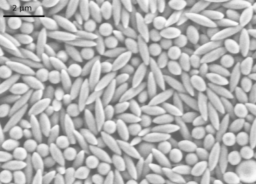
Figure 5: Scanning electron microscopy image of the stretched spheres. Most particles are approximately prolate spheroids.

The silica spherocylinders are synthesized using a modified one-pot method Chaudhary et al. (2012); Kuijk et al. (2011), and their size (as determined by scanning electron microscopy) is $1\pm 0.2$ $\mu$m by $2\pm 0.2$ $\mu$m.

We dilute the particles to a volume fraction of less than 10^-5 in an aqueous solution of glycerol (59% w/w) in water so that in the experiments, there is no more than one particle in the 120 $\times$ 120 $\times$ 100 $\mu$m imaging volume. We place approximately 5 $\mu$L of suspension in a custom sample holder and add approximately 300 $\mu$L of anhydrous decane ($\geq$99% purity, Sigma) to form the interface. The aqueous solution is refractive-index matched to the decane ($n$ = 1.41) to minimize reflections from the interface.

Taking and analyzing holograms

We capture the dynamics of the ellipsoidal particles with a digital holographic microscope. Our experimental apparatus is described in detail by Kaz et al. Kaz et al. (2012). In brief, we capture holograms with an in-line digital holographic microscope built on a Nikon TE2000-E inverted microscope. We push particles towards the interface with an out of focus optical trap ($\lambda$ = 785 nm, Thorlabs L785P090), while a laser diode ($\lambda$ = 660 nm, Thorlabs HL6545MG) illuminates them. The scattered and unscattered light interfere to form a hologram, which is collected with a 100$\times$, NA = 1.4 oil-immersion objective (Nikon) with a $n$ = 1.414-index oil to minimize spherical aberration in the hologram Kaz et al. (2012); Ovryn and Izen (2000). The holograms are then recorded with a Photon Focus MVD-1024E-160 camera at 50 $\mu$s exposure time.

We analyze the recorded holograms by fitting a light-scattering model to the data using the HoloPy package (http://manoharan.seas.harvard.edu/holopy). We have previously shown that we can use holography and an implementation of the discrete dipole approximation (A-DDA Yurkin and Hoekstra (2011)) to track non-spherical particles diffusing in water with high temporal resolution and spatial precision Wang et al. (2014). We use the same technique to analyze holograms from the spherocylinder. For the ellipsoids, we calculate the scattered field with a T-matrix solution Mishchenko and Travis (1998), which is faster than the discrete dipole approximation: calculating a 200 by 200 pixel hologram of a 0.5- by 2.0-$\mu$m ellipsoid takes 1 s using the T-matrix solution compared to 10 s with A-DDA. We use the fit results from one frame, obtained using the Levenberg-Marquardt algorithm, as the initial guess for the following frame in the time series.

To fit a time-series of holograms, we must determine good initial guesses for the parameters in the first frame, including the refractive index of the particle, its size, orientation, and position. For the refractive index we use that of bulk polystyrene ($n$ = 1.59 at 660 nm). To estimate the orientation and size of the particles, we calculate reconstructions of the hologram by Rayleigh-Kirchoff back-propagation Kreis (2002). We estimate the height from the $z$ position where the reconstruction resembles an in-focus bright-field image of the particles. We then use this reconstruction slice to estimate the particle’s size and orientation. We estimate the particle’s $x$–$y$ position using a Hough transform based algorithm in HoloPy. These estimates are then refined in the fit.

Modeling contact-line motion on the surface of a particle

To model the motion of the contact line along the surface of a spheroid, we work in the particle’s frame of reference and start from an initial position in which the particle just touches the interface at a given polar angle $\theta_{\mathrm{init}}$. To generate a trajectory that can be compared to experimental data, we choose $\theta_{\mathrm{init}}$ to be the observed polar angle of the particle just before it breaches.

The velocity of the contact line along the surface of the particle is given by

$$V=\frac{F_{\mathrm{cl}}}{\lvert F_{\mathrm{cl}}\rvert}V_{0}\exp(-U/kT+\lvert F_{\mathrm{cl}}\rvert A/2kT)$$ (3)

We define the contact line as the intersection between a plane (the interface) and the surface of a rotated prolate spheroid. For an interface at $z$=0, the contact line is given by

$$y=\pm\sqrt{a^{2}-\frac{a^{2}}{b^{2}}(-x\sin\theta+k\cos\theta)^{2}-(x\cos\theta+k\sin\theta)^{2}}$$

where $a$ and $b$ are the minor and major semi-axes of the prolate spheroid, $\theta$ is the polar angle, and $k$ is the height of the particle. In our calculations, we use 5000 points to define the contact line.

For each of the points along the contact line, we calculate the velocity from Equation 3 using $T$ = 295 K, $V_{0}$ = 1 $\mu$m/s, $U$ = 20 $kT$, $\sigma_{\mathrm{ow}}$ = 37 mN/m, and $A$ = 4 nm². We take the value for $U$ from Colosqui et al. Colosqui et al. (2013), and the values for $\sigma_{\mathrm{ow}}$ and $A$ from Kaz et al. Kaz et al. (2012). We then multiply each velocity by a time-step $\delta t$ to find the displacements $\delta l$. The $\delta l$ at each of the 5000 points are in the direction tangent to the particle. The time-steps we use are smaller in the beginning of the trajectory than at the end ($\delta t_{i}$ = $e^{-2}$, $e^{-1.98}$, $e^{-1.96}$, $...$, $e^{0}$, $...$, $e^{1.98}$, $e^{2}$) because the driving force $F_{\mathrm{cl}}$ is larger in the beginning of the trajectory. Using uniformly small time-steps for the whole integration does not change the $\theta$–$z$ trajectories, only the speed of the integration. After each time-step, we update each point along the contact line with the respective value of $\delta l$, and we fit the updated points to a plane to define the new position of the interface. The height $z$ and polar angle $\theta$ are then determined by the angle and position of the plane relative to the center of the ellipsoid.

Choice of $A$ and how it affects the velocity of the contact line

When a prolate spheroid breaches the interface, our experiments show that the contact line moves along the surface of the particle at different speeds, rotating the particle until it “lies down” at the interface. We calculate the ratio of the velocities of the slowest- to fastest-moving parts of the contact line using the following equation:

$$\frac{V_{\mathrm{center}}}{V_{\mathrm{tip}}}=\exp\left(\frac{\sigma_{\mathrm{ow}}\left(\cos\alpha_{\mathrm{D,center}}-\cos\alpha_{\mathrm{D,tip}}\right)A}{2kT}\right)$$ (4)

The ratio in equation 4 is sensitive to the dynamic contact angles $\alpha_{\mathrm{D,center}}$ and $\alpha_{\mathrm{D,tip}}$, which are set by the shape of the particles, and the value of $A$. Our group determined $A$ to be approximately 4 nm² for sulfate polystyrene particles Kaz et al. (2012), the value we use in this work, and 1-10 nm² for a range of other particles Wang et al. (2016). Boniello et al. Boniello et al. (2015) found $A$ to be on the order of 1 nm² for silica and polystyrene particles. Contact-line pinning onto nanometer-scale defects has been observed in macroscopic wetting experiments, and recent DFT simulations have shown that pinning/unpinning of the contact line on 1-nm-scale surface defects can result in macroscopic contact angle hysteresis Giacomello et al. (2016). We therefore believe choosing $A$ to be on the nanometer-scale in our simulations is justified.

If $A$ is much smaller than 1 nm², then thermal fluctuations will be comparable to the work needed to move a segment of the contact line from one defect to the next. In this situation, the contact line will have more defects to pin it. For such conditions, equation 3 may no longer provide a valid description of the motion of the contact line.

The effect of stretching the particles on their surface properties

The average slopes of the $\theta$-$z$ trajectories for our model and experimental data agree, despite our assumption that the particles have uniform surface properties. The quantitative agreement suggests that any effects from stretching the particles are not detectable to within the uncertainty of our data. This may be because the surface area of the particles did not increase very much when they were stretched to an aspect ratio of between 2.5 and 4: particles stretched to aspect ratio of 2.5 have 13% more surface area than their spherical form, and particles stretched to an aspect ratio of 4 have 28% more. An approximately 20-30% increase in surface area in parts of the particle is unlikely to alter the adsorption trajectories by much, given that the attractors for particles with $A$ = 1 and 30 nm² are not that different in slope. All of the experimental data falls between these two attractors.

We also do not expect the stretching to alter the qualitative form of the trajectories. Because the surface area of the particle increases more near its center than at its tips, the density of defects near the center should decrease relative to that near the edges, such that $A_{\mathrm{tip}}<A_{\mathrm{center}}$. Local alignment of polymer chains during stretching may also occur, leading to enhanced hydrophobicity near the center relative to the tips Coertjens et al. (2014), such that $\alpha_{\mathrm{E,tip}}<\alpha_{\mathrm{E,center}}$. Equation 3 shows that geometry and surface properties all favor $V_{\mathrm{tip}}<V_{\mathrm{center}}$, resulting in the particle pivoting as it breaches.

Direction of contact-line hops

In equation 3 we do not take into account “backward hops,” motion of the contact line in the reverse direction due to thermal fluctuations. Neglecting backward hops is a valid simplification in the regime where $\cos\alpha_{\mathrm{D}}$ is far from $\cos\alpha_{\mathrm{E}}$. When $\cos\alpha_{\mathrm{D}}$ approaches $\cos\alpha_{\mathrm{E}}$, thermal fluctuations can result in backward hops, and the model must be modified. The Supplementary Material of Kaz et al. Kaz et al. (2012) demonstrates that for the spherical (unstretched) versions of the particles that we use in this study, backward hops can be neglected so long as the dynamic contact angle is more than 0.01 radians from the equilibrium contact angle. Therefore in this work, we consider only the regime where forward-hopping dominates.

MOVIE-ellipsoid_holo_rendering_4xslower.avi

Holograms and three-dimensional renderings of a 0.3 $\times$ 1.1 $\mu$m ellipsoid breaching an oil-water interface from the aqueous phase. Playback is slower than real time by a factor of 4.

References

- Huh and Scriven (1971) C. Huh and L. E. Scriven, Journal of Colloid and Interface Science 35, 85 (1971).
- Dussan V. and Davis (1974) E. B. Dussan V. and S. H. Davis, Journal of Fluid Mechanics 65, 71 (1974).
- de Gennes (1985) P. G. de Gennes, Reviews of Modern Physics 57, 827 (1985).
- Blake and Haynes (1969) T. D. Blake and J. M. Haynes, Journal of Colloid and Interface Science 30, 421 (1969).
- Blake (2006) T. D. Blake, Journal of Colloid and Interface Science 299, 1 (2006).
- Brochard-Wyart and de Gennes (1992) F. Brochard-Wyart and P. G. de Gennes, Advances in Colloid and Interface Science 39, 1 (1992).
- Snoeijer and Andreotti (2013) J. H. Snoeijer and B. Andreotti, Annual Review of Fluid Mechanics 45, 269 (2013).
- Prevost et al. (1999) A. Prevost, E. Rolley, and C. Guthmann, Physical Review Letters 83, 348 (1999).
- Rolley and Guthmann (2007) E. Rolley and C. Guthmann, Physical Review Letters 98, 166105 (2007).
- Giacomello et al. (2016) A. Giacomello, L. Schimmele, and S. Dietrich, Proceedings of the National Academy of Sciences 113, E262 (2016).
- Günther et al. (2014) F. Günther, S. Frijters, and J. Harting, Soft Matter 10, 4977 (2014).
- de Graaf et al. (2010) J. de Graaf, M. Dijkstra, and R. van Roij, The Journal of Chemical Physics 132, 164902 (2010).
- (13) See Supplemental Material [URL], which includes Refs. Ho et al. (1993); Yunker et al. (2011); Chaudhary et al. (2012); Kuijk et al. (2011); Ovryn and Izen (2000); Yurkin and Hoekstra (2011); Wang et al. (2014); Kreis (2002), for details of sample preparation, analysis methods, and movies.
- Binks (2007) B. Binks, Physical Chemistry Chemical Physics 9, 6298 (2007).
- Pieranski (1980) P. Pieranski, Physical Review Letters 45, 569 (1980).
- Aveyard et al. (2000) R. Aveyard, J. H. Clint, D. Nees, and V. N. Paunov, Langmuir 16, 1969 (2000).
- Zahn and Maret (2000) K. Zahn and G. Maret, Physical Review Letters 85, 3656 (2000).
- Bausch et al. (2003) A. R. Bausch, M. J. Bowick, A. Cacciuto, A. D. Dinsmore, M. F. Hsu, D. R. Nelson, M. G. Nikolaides, A. Travesset, and D. A. Weitz, Science 299, 1716 (2003).
- König et al. (2005) H. König, R. Hund, K. Zahn, and G. Maret, The European Physical Journal E 18, 287 (2005).
- Cavallaro et al. (2011) M. Cavallaro, L. Botto, E. P. Lewandowski, M. Wang, and K. J. Stebe, Proceedings of the National Academy of Sciences 108, 20923 (2011).
- Botto et al. (2012) L. Botto, L. Yao, R. L. Leheny, and K. J. Stebe, Soft Matter 8, 4971 (2012).
- Paunov and Cayre (2004) V. Paunov and O. Cayre, Advanced Materials 16, 788 (2004).
- Retsch et al. (2009) M. Retsch, Z. Zhou, S. River, M. Kappl, X. S. Zhao, U. Jonas, and Q. Li, Macromolecular Chemistry and Physics 210, 230 (2009).
- Isa et al. (2010) L. Isa, K. Kumar, M. Müller, J. Grolig, M. Textor, and E. Reimhult, ACS Nano 4, 5665 (2010).
- Ramsden (1903) W. Ramsden, Proceedings of the Royal Society of London 72, 156 (1903).
- Pickering (1907) S. U. Pickering, Journal of the Chemical Society 91, 2001 (1907).
- Dinsmore et al. (2002) A. Dinsmore, M. F. Hsu, M. Nikolaides, M. Marquez, A. Bausch, and D. Weitz, Science 298, 1006 (2002).
- McGorty et al. (2010) R. McGorty, J. Fung, D. Kaz, and V. N. Manoharan, Materials Today 13, 34 (2010).
- Wang et al. (2016) A. Wang, R. McGorty, D. M. Kaz, and V. N. Manoharan, Soft Matter 12, 8958 (2016).
- Kralchevsky et al. (2001) P. A. Kralchevsky, N. D. Denkov, and K. D. Danov, Langmuir 17, 7694 (2001).
- Sharifi-Mood et al. (2015) N. Sharifi-Mood, I. B. Liu, and K. J. Stebe, Soft Matter 11, 6768 (2015).
- Boniello et al. (2015) G. Boniello, C. Blanc, D. Fedorenko, M. Medfai, N. B. Mbarek, M. In, M. Gross, A. Stocco, and M. Nobili, Nature Materials 14, 908 (2015).
- Kaz et al. (2012) D. M. Kaz, R. McGorty, M. Mani, M. P. Brenner, and V. N. Manoharan, Nature Materials 11, 138 (2012).
- Colosqui et al. (2013) C. E. Colosqui, J. F. Morris, and J. Koplik, Physical Review Letters 111, 028302 (2013).
- Coertjens et al. (2014) S. Coertjens, P. Moldenaers, J. Vermant, and L. Isa, Langmuir 30, 4289 (2014).
- Mihiretie (2013) B. Mihiretie, Mechanical effects of light on anisotropic micron-sized particles and their wetting dynamics at the water-air interface, Ph.D. thesis, Université de Bordeaux 1 (2013).
- Mishchenko and Travis (1998) M. I. Mishchenko and L. D. Travis, Journal of Quantitative Spectroscopy and Radiative Transfer 60, 309 (1998).
- Loudet et al. (2005) J. C. Loudet, A. M. Alsayed, J. Zhang, and A. G. Yodh, Physical Review Letters 94, 018301 (2005).
- Ho et al. (1993) C. Ho, A. Keller, J. Odell, and R. Ottewill, Colloid and Polymer Science 271, 469 (1993).
- Yunker et al. (2011) P. J. Yunker, T. Still, M. A. Lohr, and A. G. Yodh, Nature 476, 308 (2011).
- Chaudhary et al. (2012) K. Chaudhary, Q. Chen, J. J. Juárez, S. Granick, and J. A. Lewis, Journal of the American Chemical Society 134, 12901 (2012).
- Kuijk et al. (2011) A. Kuijk, A. van Blaaderen, and A. Imhof, Journal of the American Chemical Society 133, 2346 (2011).
- Ovryn and Izen (2000) B. Ovryn and S. H. Izen, Journal of the Optical Society of America A 17, 1202 (2000).
- Yurkin and Hoekstra (2011) M. A. Yurkin and A. G. Hoekstra, Journal of Quantitative Spectroscopy and Radiative Transfer 112, 2234 (2011).
- Wang et al. (2014) A. Wang, T. G. Dimiduk, J. Fung, S. Razavi, I. Kretzschmar, K. Chaudhary, and V. N. Manoharan, Journal of Quantitative Spectroscopy and Radiative Transfer 146, 499 (2014).
- Kreis (2002) T. M. Kreis, Optical Engineering 41, 1829 (2002).