Anderson transition of cold atoms with synthetic spin-orbit coupling in two-dimensional speckle potentials

Abstract

We investigate the metal-insulator transition occurring in two dimensional (2D) systems of noninteracting atoms in the presence of artificial spin-orbit interactions and a spatially correlated disorder generated by laser speckles. Based on a high order discretization scheme, we calculate the precise position of the mobility edge and verify that the transition belongs to the symplectic universality class. We show that the mobility edge depends strongly on the mixing angle between Rashba and Dresselhaus spin-orbit couplings. For equal couplings a non-power-law divergence is found, signaling the crossing to the orthogonal class, where such a 2D transition is forbidden.

Anderson localization (AL) Anderson (1958), namely the absence of diffusion of a coherent wave in a disordered medium due to the interference between multiple-scattering paths, is a general phenomenon observed for several kinds of waves, including light waves in diffusive media Wiersma et al. (1997); Störzer et al. (2006) or photonic crystals Schwartz et al. (2007); Lahini et al. (2008), ultrasound Hu et al. (2008), microwaves Chabanov et al. (2000) and atomic matter waves Moore et al. (1995); Billy et al. (2008); Roati et al. (2008), the latter describing the behavior of atoms in the low-temperature quantum regime.

Since AL finds its origin on interference effects, the space dimension as well as the symmetries of the model play a crucial role Evers and Mirlin (2008). When both spin-rotational and time-reversal symmetries are preserved, the system belongs to the orthogonal universality class. While AL is the generic scenario in one and two dimensions, in higher dimensions an Anderson phase transition occurs at a critical value of the energy $E=E_{c}$, called the mobility edge, separating localized states at lower energy from diffusive states at higher energy.

The inclusion of spin-orbit coupling (SOC) breaks SU(2) invariance and drives the system towards the symplectic universality class. The spin of the particle rotates as the latter moves around a closed loop and the direct and the time-reversed paths (on average) interfere destructively rather than constructively, favoring diffusion rather than localization Hikami et al. (1980). This spin-interference effect, called (weak) antilocalization, has already been observed for 2D electron gases in semiconductor quantum wells or at the surface of topological insulators. A distinctive feature of the symplectic class is the occurrence of a 2D Anderson transition Ando (1989); Fastenrath et al. (1991); Sheng et al. (2005) for strong SOC, but its experimental evidence is still lacking.

Ultracold atoms are natural candidates to fill the gap. Effects from atom-atom interaction can be reduced via Feshbach resonances and a tunable random potential can be generated from laser speckles Sanchez-Palencia and Lewenstein (2010). Thus far experiments have focused on the orthogonal class. Recent achievements include the observation Jendrzejewski et al. (2012a) of coherent backscattering in 2D systems and the study Kondov et al. (2011); Jendrzejewski et al. (2012b); Semeghini et al. (2015) of the mobility edge for the 3D Anderson transition. From the theoretical front, accurate numerical calculations Delande and Orso (2014); Fratini and Pilati (2015a); Pasek et al. (2015); Fratini and Pilati (2015b) for $E_{c}$ have appeared going beyond approximate estimates Kuhn et al. (2007); Yedjour and Tiggelen (2010); Piraud et al. (2013). Atomic gases have also been employed to realize experimentally the quantum kicked rotor model and study AL in momentum space. This setup has allowed a detailed investigation Chabé et al. (2008); Lopez et al. (2012) of the 3D Anderson transition and the observation of 2D AL  Manai et al. (2015). Parallel to these developments, significant experimental and theoretical progress has been made to create and control artificial SOC for cold atoms with the aim of exploring topological phases of quantum matter (for a review, see Galitski and Spielman (2013); Zhai (2015)). Very recently, a synthetic SOC with tunable Rashba Bychkov and Rashba (1984) and Dresselhaus Dresselhaus (1955) terms has been experimentally realized Huang et al. (2016) in 2D atomic gases, opening a new avenue to explore Anderson transitions in the symplectic class.

In this Letter we investigate the 2D Anderson transition in atomic gases with artificial SOC and subject to a laser speckle potential. We calculate numerically the precise position of the mobility edge, taking into full account the potential distribution and the spatial correlations of the disorder. In particular: (i) we identify a regime where $E_{c}$ depends linearly on the disorder amplitude, with a slope decreasing and changing sign as the SOC increases (Fig.2); (ii) we show that the interference between Rashba and Dresselhauss SOC leads to a strong dependence of $E_{c}$ on the mixing angle with a non-power-law divergence as the two magnitudes coincide (Fig.3). Hence, by tuning the SOC one can induce an interesting crossover between symplectic and orthogonal universality classes.

Previous theoretical studies of atomic gases in the presence of both disorder and SOC have addressed AL in 1D quasiperiodic lattices Zhou et al. (2013), the dynamics of a 1D Bose-Einstein condensate Mardonov et al. (2015) and the competition between disorder and superfluidity in 2D Fermi gases Liu et al. (2016).

The Hamiltonian of a spin-1/2 atom of mass $m$ in the presence of linear SOC is given by:

$$H=\left(\frac{\mathbf{k}^{2}}{2m}+V(\mathbf{r})\right)\mathds{1}+\lambda_{R}(k_{y}\sigma_{x}-k_{x}\sigma_{y})+\lambda_{D}(k_{y}\sigma_{x}+k_{x}\sigma_{y}),$$ (1)

where $\mathbf{k}=-i\nabla$ is the momentum of the particle (we use the convention $\hbar=1$) and $V(\mathbf{r})$ is the external speckle potential. Moreover $\mathds{1}$ is the $2\times 2$ identity matrix, $\sigma_{x},\sigma_{y}$ are the Pauli matrices and $\lambda_{R}$ and $\lambda_{D}$ correspond to the strengths of the Rashba and Dresselhaus couplings, respectively (for a discussion about realistic schemes to implement such a model with cold atoms see Ref. Campbell et al. (2011)). In the absence of disorder, a pure Rashba coupling yields split energy dispersions $E_{\mathbf{k}\pm}=k^{2}/2m\pm k\lambda_{R}$, with $k=|\mathbf{k}|$. The ground state occurs at $k=m\lambda_{R}$ with energy $-m\lambda_{R}^{2}/2$.

In the following we shall focus on blue-detuned speckles, as employed in recent experiments Kondov et al. (2011); Jendrzejewski et al. (2012b); Semeghini et al. (2015). Their potential distribution follows the Rayleigh law Kuhn et al. (2005); Goodman (2007):

$$P(V)=\frac{\Theta(V+V_{0})}{V_{0}}\exp{\left(-\frac{V+V_{0}}{V_{0}}\right)}$$ (2)

where $\Theta$ is the Heaviside (unit step) function and $V_{0}$ is related to the variance by $\langle V^{2}\rangle\!=\!V_{0}^{2}$. Notice that in Eq.(2) we have shifted the potential by its average value, without loss of generality.

We generate the speckle potential numerically by first computing the normalized electric field amplitude $\epsilon(\mathbf{r})$, whose real and imaginary parts are normally distributed random variables with zero mean and unit variance. This quantity is then convoluted with the point spread function $h(\mathbf{r})$ of the diffusive glass plate. Let us call $f(\mathbf{r})$ the modulus square of the result; that is, $f(\mathbf{r})=|\int d\mathbf{r}^{\prime}\epsilon(\mathbf{r}^{\prime})h(\mathbf{r}-\mathbf{r}^{\prime})|^{2}$. Then the disorder potential is given by $V(\mathbf{r})=V_{0}(f(\mathbf{r})/f_{\textrm{av}}-1)$, where $f_{\textrm{av}}=\int d\mathbf{r}f(\mathbf{r})/S$ is the spatial average of $f$, with $S$ being the surface area.

The spatial correlation function of the 2D speckle pattern can be written as $\langle V(0)V(\mathbf{r})\rangle=V_{0}^{2}|h(\mathbf{r})/h(0)|^{2}$. For a circular aperture, the Fourier transform of the point spread function is an Airy disk, $\tilde{h}(\mathbf{k})=\Theta(k_{0}-|\mathbf{k}|)$, where $k_{0}=\alpha k_{L}$, $\alpha$ being the aperture angle and $k_{L}$ the wavevector of the laser beam. By using $\int_{0}^{2\pi}e^{-ikr\cos\theta}d\theta=2\pi J_{0}(kr)$ and $\int_{0}^{k_{0}}J_{0}(kr)kdk=J_{1}(k_{0}r)k_{0}/r$, $J_{n}(x)$ being the Bessel function of order $n$, we obtain

$$\langle V(0)V(\mathbf{r})\rangle=V_{0}^{2}\frac{4J_{1}^{2}(r/\sigma)}{(r/\sigma)^{2}},$$ (3)

where $\sigma=1/k_{0}$ is the correlation length of the speckle pattern (see Supplemental Material ). In the following we measure all energies in units of the correlation energy $E_{\sigma}=1/(m\sigma^{2})$.

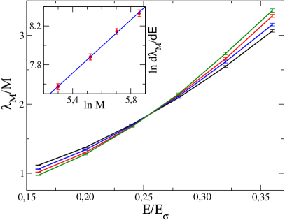
Figure 1: (color online) Numerical calculation of the critical point of the 2D Anderson transition for cold atoms with synthetic Rashba SOC in a blue-detuned speckle. After discretization of the model on a strip-shaped grid of spacing $\Delta$, height $M$ and length $L\gg M$, we use the transfer-matrix method to calculate the localization length $\lambda_{M}$. The main panel shows the ratio $\lambda_{M}/M$ as a function of energy calculated for increasing values of $M=200$ (top curve on the left), $250,300,350$ assuming $\Delta=0.2\pi\sigma$. The crossing point corresponds to the mobility edge, $E=E_{c}\simeq 0.256E_{\sigma}$, with $E_{\sigma}=1/(m\sigma^{2})$, $\sigma$ being the correlation length of the speckle; see Eq.(3). The Rashba strength is $m\lambda_{R}\sigma=0.03$ and the disorder amplitude is $V_{0}\!=\!E_{\sigma}$. The inset shows the evaluation of the critical exponent $\nu$ from the scaling behavior of $d\lambda_{M}/dE$ at the mobility edge, see Eq.(5).

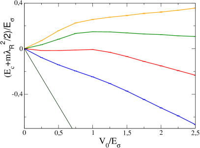
Figure 2: (color online) Mobility edge $E_{c}$ of the 2D Anderson transition separating low-energy localized states $(E<E_{c})$ from high-energy diffusive states $(E>E_{c})$, plotted as a function of the disorder amplitude $V_{0}$ and for increasing values of the Rashba spin-orbit coupling $\lambda_{R}m\sigma=0.03\;\textrm{(top curve)},0.1,0.3$ and $1.256$, assuming $\lambda_{D}=0$. The black line corresponds to the energy bottom $E=-V_{0}-m\lambda_{R}^{2}/2$, below which no single particle state exists. Notice the linear behavior of $E_{c}$ for $V_{0}/E_{\sigma}\gtrsim 1$.

In order to calculate the precise position of the mobility edge, we discretize the stationary Schrodinger equation, $H\Psi=E\Psi$, on a grid by replacing first and second order derivates by finite differences. Here $\Psi=(\psi_{\uparrow}\psi_{\downarrow})^{t}$ is the two-component spinor wave function and $E$ is the energy of the particle. The simplest procedure, as employed in Ref.Delande and Orso (2014), is to use the second order central approximation: $\partial_{x}\psi_{\sigma}=(\psi_{i+1j\sigma}-\psi_{i-1j\sigma})/(2\Delta)+\mathcal{O}(\Delta^{2})$ and $\partial_{xx}\psi_{\sigma}=(\psi_{i+1j\sigma}+\psi_{i-1j\sigma}-2\psi_{ij\sigma})/\Delta^{2}+\mathcal{O}(\Delta^{2})$ (and analogously for the $y$ variable). Here $\psi_{ij\sigma}\equiv\psi_{\sigma}(\mathbf{r}=\Delta i\mathbf{e}_{x}+\Delta j\mathbf{e}_{y})$, $\mathbf{e}_{x}$ and $\mathbf{e}_{y}$ being the unitary vector along the $x$ and $y$ axes, respectively, and $\Delta$ the discretization step. This turned out to be unpractical for strong SOC, as it requires very fine grids to get converged results for the transmission amplitude, increasing significantly the computational effort (see Supplemental Material). For this reason, we have used the fourth order approximation: $\partial_{x}\psi_{\sigma}=(-\psi_{i+2j\sigma}+\psi_{i-2j\sigma}+8\psi_{i+1j\sigma}-8\psi_{i-1j\sigma})/(12\Delta)+\mathcal{O}(\Delta^{4})$ and $\partial_{xx}\psi_{\sigma}=(-\psi_{i+2j\sigma}-\psi_{i-2j\sigma}+16\psi_{i+1j\sigma}+16\psi_{i-1j\sigma}-30\psi_{ij\sigma})/(12\Delta^{2})+\mathcal{O}(\Delta^{4})$.

The retained scheme yields a generalized 2D Anderson model, where the coupling also extends to next-to-nearest neighboring sites. We consider a strip-shaped grid with $L$ sites in the longitudinal direction and $M$ sites in the transverse one, with $M\!\ll\!L$. We also impose periodic boundary condition in the transverse direction to reduce finite-size effects. In this quasi-1D geometry, the system is Anderson localized and we use the transfer matrix method McKinnon and Kramer (1983) to accurately compute its transmission amplitude $T$. For large $L$, the latter decays exponentially as $T\propto\exp(-2L/\lambda_{M})$, $\lambda_{M}$ being the 1D localization length.

The critical point of the Anderson transition can be identified by calculating the ratio $\lambda_{M}/M$ as a function of energy and for increasing values of $M$, as shown in Fig. 1 (main panel). Here we have considered a pure Rashba SOC with strength $\lambda_{R}m\sigma=0.03$ and disorder amplitude $V_{0}\!=\!E_{\sigma}$. The grid spacing is $\Delta=0.2\pi\sigma$ and $M$ varies between $200$ and $350$. Since the log of the total transmission is a self-averaging quantity, we have calculated it for grids of length $L=50000$ using $336$ different realizations of the disorder, and then averaging the obtained results. In this way the relative error in the 1D localization length is below $0.7\%$.

At low energy, in the localized regime, $\lambda_{M}$ converges to the 2D localization length $\xi=\lim_{M\to\infty}\lambda_{M}$ as $M$ becomes large, implying that the ratio $\lambda_{M}/M$ decreases with $M$. In contrast, at high energy, in the metallic phase, $\lambda_{M}/M$ increases with $M$, whereas at the critical point, the ratio takes a (finite) constant value, $\lim_{M\rightarrow+\infty}\lambda_{M}/M=\Lambda_{c}$. From the crossing point in Fig. 1, we find $E_{c}\simeq 0.256E_{\sigma}$ and $\Lambda_{c}\simeq 1.85$.

Next, we show that the 2D Anderson transition discussed here belongs to the symplectic class. According to the one parameter scaling theory, the ratio $\lambda_{M}/M$ can be written in terms of a scaling function $f$ as

$$\frac{\lambda_{M}(E)}{M}=f(u(\omega)M^{1/\nu}),$$ (4)

where $u$ is a function of the reduced energy $\omega=(E-E_{c})/E_{c}$ and $\nu$ is the critical exponent. In Eq.(4) we have neglected possible contributions coming from irrelevant terms, since our values of $M$ are relatively large and no sizable drift of the crossing point is observed in Fig. 1.

A first estimate of the critical exponent can be obtained by linearizing the functions $f$ and $u$ in the proximity of the mobility edge. By substituting $f(x)=a_{0}+x$ and $u(\omega)=b_{1}\omega$ in Eq.(4), where $a_{0}$ and $b_{1}$ are unknown constants, and taking the derivative of both sides with respect to the energy, we obtain that at the critical point

$$\frac{d\lambda_{M}}{dE}=\frac{b_{1}}{E_{c}}M^{1+1/\nu}.$$ (5)

We calculate the derivative in Eq.(5) via central difference using our numerical data at $E=0.24E_{\sigma}$ and $E=0.28E_{\sigma}$, taking into account their statistical uncertainty. The result is then plotted in the inset of Fig. 1 as a function of $M$, using a log-log scale. By fitting the data with a straight line of slope $1+1/\nu$, we find $\nu=2.69\pm 0.21$, which is fully consistent with the best available Asada et al. (2002, 2004) estimate $\nu=2.73\pm 0.02$ for the 2D Anderson transition in the symplectic class obtained in lattice models with random SOC.

We can further improve the accuracy of our results by using the entire numerical data set. For this purpose, the functions $u$ and $f$ are Taylor expanded up to order $m$ and $n$, respectively, yielding $u(\omega)=\sum_{j=1}^{m}b_{j}\omega^{j}$ and $f(x)=\sum_{k=0}^{n}a_{k}x^{k}$, with $a_{1}=1$. The total number of fitting parameters is then given by $2+m+n$. Following Ref. Slevin and Ohtsuki (2014), we perform a nonlinear least squares fit of the data, to extract the best estimates for the fitting parameters and their error bars. With $n=m=3$ we obtain $E_{c}/E_{\sigma}=0.256\pm 0.002$, $\nu=2.67\pm 0.14$ and $a_{0}=\Lambda_{c}=1.855\pm 0.02$, corresponding to a reduced chi square $\chi_{\textrm{red}}=0.32$. Similar results can be found using smaller values of $m$ and $n$, by narrowing the fitting region around the mobility edge. Notice that, for fixed periodic boundary conditions and in the absence of discretization effects, $\Lambda_{c}$ is also universal. Our result compares well with the value $\Lambda_{c}=1.844\pm 0.002$ obtained in Refs. Asada et al. (2002, 2004), suggesting that discretization effects are indeed rather small.

In Fig. 2 we show the calculated mobility edge as a function of $V_{0}$ for increasing values of $\lambda_{R}$, going from $m\lambda_{R}\sigma=0.03$ (top curve) to $m\lambda_{R}\sigma=1.256$ (the inclusion of the Dresselhaus term will be discussed later). For vanishing SOC and finite disorder strength all states are localized and $E_{c}\rightarrow+\infty$. We see in Fig. 2 that the mobility edge exhibits a kink around $V_{0}\sim E_{\sigma}$ followed by an approximately linear behavior in the strong disorder regime, which is reminiscent of classical percolation. Remarkably, the slope depends on the value of the Rashba SOC, changing continuously from positive to negative values as $\lambda_{R}$ increases. In contrast, for strong SOC, $E_{c}$ always decreases as $V_{0}$ increases, a situation already encountered for atoms in blue-detuned 3D laser speckles Delande and Orso (2014); Fratini and Pilati (2015a) without SOC.

Notice that discretization effects become more and more important as $\lambda_{R}$ increases (for $\lambda_{R}m\sigma=1.256$ we have used $\Delta=0.15\pi\sigma$). Indeed the grid spacing must satisfy $\Delta\ll\textrm{min}(\sigma,\ell_{\textrm{so}})$, where $\ell_{\textrm{so}}=\pi/(m\lambda_{R})$ is the spin-precession length. For strong SOC, $\ell_{\textrm{so}}$ becomes the shortest length scale in the problem, implying that very fine grids are needed to accurately compute the position of the mobility edge. Altogether, data shown in Fig. 2 required $700000$ h of allocation time on a supercomputer with $2$ Pflop/s.

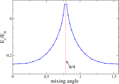
Figure 3: (color online) Mobility edge as a function of the mixing angle $\theta=\arctan(\lambda_{D}/\lambda_{R})$ between Rashba and Dresselhaus SOC, for a fixed value of the total strength $\sqrt{\lambda_{R}^{2}+\lambda_{D}^{2}}m\sigma=0.5$ and disorder amplitude $V_{0}=E_{\sigma}$. Approaching $\theta=\pi/4$ (vertical dashed line), corresponding to equal strengths of Rashba and Dresselhaus SOC, the mobility edge rises sharply and actually diverges. Indeed, at this special point, spin scattering is absent and the model falls into the orthogonal universality class, for which all states are localized in two dimensions implying $E_{c}=+\infty$. Notice that the mobility edge $E_{c}$ is invariant under the transformation $\theta\rightarrow\pi/2-\theta$ exchanging the Rashba and Dresselhaus terms in Eq.(1).

Thus far, we have mainly focused on a pure Rashba SOC by setting $\lambda_{D}=0$, but the same results hold for a pure Dresselhaus SOC of the same strength. Indeed, the transformation $k_{x}\rightarrow-k_{x}$ in Eq.(1) interchanges the Rashba and the Dresselhaus terms, leaving the total Hamiltonian invariant. Let us now investigate the behavior of the mobility edge when both terms are present and interfere between each other (weak antilocalization contributions to conductivity from Rashba and Dresselhaus SOC are indeed not additive, see Ref. Pikus and Pikus (1995)). For this we write $\lambda_{R}=v_{\textrm{so}}\cos\theta$ and $\lambda_{D}=v_{\textrm{so}}\sin\theta$, where $v_{\textrm{so}}=\sqrt{\lambda_{R}^{2}+\lambda_{D}^{2}}$ and $\theta=\arctan(\lambda_{D}/\lambda_{R})$ is the mixing angle. In Fig.3 we show the position of the mobility edge as a function of the mixing angle for $v_{\textrm{so}}=0.5/m\sigma$ and $V_{0}=E_{\sigma}$. Since $E_{c}$ is invariant under the transformation $\theta\rightarrow\pi/2-\theta$, it is sufficient to study it for $\theta$ varying between $0$ (pure Rashba) and $\pi/4$ (equal strengths of Rashba and Dresselhaus SOC). At $\theta=\pi/4$ the system is known Bernevig et al. (2006); Koralek et al. (2009) to exhibit an exact SU(2) symmetry, which generates persistent spin-helix states and is robust against spin-independent disorder.

We see in Fig.3 that the mobility edge is strongly dependent on the mixing angle and diverges as $\theta$ approaches $\pi/4$. Indeed for $\lambda_{R}=\lambda_{D}$ the SOC term in Eq.(1) reduces to $2\lambda_{R}k_{y}\sigma_{x}$. Since $\sigma_{x}$ is Hermitian and commutes with $H$, we can find common eigenstates for the two operators. Taking into account that the eigenvalues of $\sigma_{x}$ are $\epsilon_{\pm}=\pm 1$, the Hamiltonian decouples into two scalar sectors, $H_{\pm}=(\mathbf{k}^{2}/2m+V(\mathbf{r}))\pm 2\lambda_{R}k_{y}$, implying that spin scattering is absent and the 2D model belongs to the orthogonal class, for which all states are localized and $E_{c}=+\infty$.

A very interesting and novel question concerns the nature (power law, logarithmic, etc.) of the divergence observed in Fig.3. According to Wegner’s theory Wegner (1986) (see also Ref. Jung et al. (2016)), which holds for quantum models in $2+\epsilon$ spatial dimensions, a small term breaking either the spin-rotational or the time-reversal symmetries induces a shift of the mobility edge which is a power law with exponent equal to $1/(2\nu_{\textrm{orth}})$, $\nu_{\textrm{orth}}$ being the critical exponent in the orthogonal class. In our 2D case $\nu_{\textrm{orth}}\rightarrow+\infty$, so $E_{c}$ cannot diverge as a power-law of $|\lambda_{R}-\lambda_{D}|$. The divergence is probably logarithmic, but proving it requires further numerical and/or analytical work.

In conclusion, we have shown that atoms with artificial Rashba and Dresselhaus SOC exposed to a 2D speckle potential undergo an Anderson transition belonging to the symplectic universality class. We have computed the precise position of the mobility edge and identified a regime (Fig. 2) where the latter scales linearly as a function of the disorder strength, with a slope changing sign as the SOC increases. Importantly, we have unveiled (Fig. 3) that the mobility edge exhibits a non-power-law divergence at the spin-helix point, reflecting the crossover to the orthogonal class. Our results call for the extension of Wegner’s theory Wegner (1986) to pure 2D systems, which by itself is a novel and interesting theoretical challenge.

Our predictions can already be tested experimentally using ultracold atoms with tunable synthetic SOC. Finally, we mention that the numerical approach developed here is completely general and can be applied to any kind of random potential, including short range Morong and DeMarco (2015).

We thank D. Delande and V. Josse for useful discussions. We also thank K. Slevin and T. Ohtsuki for correspondence and for drawing our attention to Refs. Wegner (1986); Jung et al. (2016). This work was granted access to the HPC resources of TGCC under the allocations 2015-057301 and 2016-057629 made by GENCI (Grand Equipement National de Calcul Intensif).

References

- Anderson (1958) P. W. Anderson, Phys. Rev. 109, 1492 (1958).
- Wiersma et al. (1997) D. S. Wiersma, P. Bartolini, A. Lagendijk, and R. Righini, Nature (London) 390, 671 (1997).
- Störzer et al. (2006) M. Störzer, P. Gross, C. M. Aegerter, and G. Maret, Phys. Rev. Lett. 96, 063904 (2006).
- Schwartz et al. (2007) T. Schwartz, G. Bartal, S. Fishman, and B. Segev, Nature (London) 446, 52 (2007).
- Lahini et al. (2008) Y. Lahini, A. Avidan, F. Pozzi, M. Sorel, R. Morandotti, D. N. Christodoulides, and Y. Silberberg, Phys. Rev. Lett. 100, 013906 (2008).
- Hu et al. (2008) H. Hu, A. Strybulevych, J. H. Page, S. E. Skipetrov, and B. A. van Tiggelen, Nat. Phys. 4, 945 (2008).
- Chabanov et al. (2000) A. A. Chabanov, M. Stoytchev, and A. Z. Genack, Nature (London) 404, 850 (2000).
- Moore et al. (1995) F. L. Moore, J. C. Robinson, C. F. Bharucha, B. Sundaram, and M. G. Raizen, Phys. Rev. Lett. 75, 4598 (1995).
- Billy et al. (2008) J. Billy, V. Josse, Z. Zuo, A. Bernard, B. Hambrecht, P. Lugan, D. Clément, L. Sanchez-Palencia, P. Bouyer, and A. Aspect, Nature (London) 453, 891 (2008).
- Roati et al. (2008) G. Roati, C. d’Errico, L. Fallani, M. Fattori, C. Fort, M. Zaccanti, G. Modugno, M. Modugno, and M. Inguscio, Nature (London) 453, 895 (2008).
- Evers and Mirlin (2008) F. Evers and A. D. Mirlin, Rev. Mod. Phys. 80, 1355 (2008).
- Hikami et al. (1980) S. Hikami, A. I. Larkin, and Y. Nagaoka, Prog. Theor. Phys. 63, 707 (1980).
- Ando (1989) T. Ando, Phys. Rev. B 40, 5325 (1989).
- Fastenrath et al. (1991) U. Fastenrath, G. Adams, R. Bundschuh, T. Hermes, B. Raab, I. Schlosser, T. Wehner, and T. Wichmann, Physica A 172, 302 (1991).
- Sheng et al. (2005) L. Sheng, D. N. Sheng, and C. S. Ting, Phys. Rev. Lett. 94, 016602 (2005).
- Sanchez-Palencia and Lewenstein (2010) L. Sanchez-Palencia and M. Lewenstein, Nat. Phys. 6, 87 (2010).
- Jendrzejewski et al. (2012a) F. Jendrzejewski, K. Muller, J. Richard, A. Date, T. Plisson, P. Bouyer, A. Aspect, and V. Josse, Phys. Rev. Lett. 109, 195302 (2012a).
- Kondov et al. (2011) S. S. Kondov, W. R. McGehee, J. J. Zirbel, and B. DeMarco, Science 334, 66 (2011).
- Jendrzejewski et al. (2012b) F. Jendrzejewski, A. Bernard, K. Muller, P. Cheinet, V. Josse, M. Piraud, L. Pezzé, L. Sanchez-Palencia, A. Aspect, and P. Bouyer, Nat. Phys. 8, 398 (2012b).
- Semeghini et al. (2015) G. Semeghini, M. Landini, P. Castilho, S. Roy, G. Spagnolli, A. Trenkwalder, M. Fattori, M. Inguscio, and G. Modugno, Nat. Phys. 11, 554 (2015).
- Delande and Orso (2014) D. Delande and G. Orso, Phys. Rev. Lett. 113, 060601 (2014).
- Fratini and Pilati (2015a) E. Fratini and S. Pilati, Phys. Rev. A 91, 061601 (2015a).
- Pasek et al. (2015) M. Pasek, Z. Zhao, D. Delande, and G. Orso, Phys. Rev. A 92, 053618 (2015).
- Fratini and Pilati (2015b) E. Fratini and S. Pilati, Phys. Rev. A 92, 063621 (2015b).
- Kuhn et al. (2007) R. Kuhn, O. Sigwarth, C. Miniatura, D. Delande, and C. Müller, New J. Phys. 9, 161 (2007).
- Yedjour and Tiggelen (2010) A. Yedjour and B. A. Tiggelen, Eur. Phys. J. D 59, 249 (2010).
- Piraud et al. (2013) M. Piraud, L. Pezzé, and L. Sanchez-Palencia, New Journal of Physics 15, 075007 (2013).
- Chabé et al. (2008) J. Chabé, G. Lemarié, B. Grémaud, D. Delande, P. Szriftgiser, and J. C. Garreau, Phys. Rev. Lett. 101, 255702 (2008).
- Lopez et al. (2012) M. Lopez, J.-F. Clément, P. Szriftgiser, J. C. Garreau, and D. Delande, Phys. Rev. Lett. 108, 095701 (2012).
- Manai et al. (2015) I. Manai, J.-F. Clément, R. Chicireanu, C. Hainaut, J. C. Garreau, P. Szriftgiser, and D. Delande, Phys. Rev. Lett. 115, 240603 (2015).
- Galitski and Spielman (2013) V. Galitski and I. B. Spielman, Nature 494, 49 (2013).
- Zhai (2015) H. Zhai, Rep. Prog. Phys. 78, 026001 (2015).
- Bychkov and Rashba (1984) Y. A. Bychkov and E. I. Rashba, J. Phys. C 17, 6039 (1984).
- Dresselhaus (1955) G. Dresselhaus, Phys. Rev. 100, 580 (1955).
- Huang et al. (2016) L. Huang, Z. Meng, P. Wang, P. Peng, S.-L. Zhang, L. Chen, D. Li, Q. Zhou, and J. Zhang, Nat. Phys. 12, 540 (2016).
- Zhou et al. (2013) L. Zhou, H. Pu, and W. Zhang, Phys. Rev. A 87, 023625 (2013).
- Mardonov et al. (2015) S. Mardonov, M. Modugno, and E. Y. Sherman, Phys. Rev. Lett. 115, 180402 (2015).
- Liu et al. (2016) S. Liu, X. F. Zhou, G. C. Guo, and Y. S. Zhang, Sci. Rep. 6, 22623 (2016).
- Campbell et al. (2011) D. L. Campbell, G. Juzeliunas, and I. B. Spielman, Phys. Rev. A 84, 025602 (2011).
- Kuhn et al. (2005) R. C. Kuhn, C. Miniatura, D. Delande, O. Sigwarth, and C. A. Müller, Phys. Rev. Lett. 95, 250403 (2005).
- Goodman (2007) J. Goodman, Speckle Phenomena in Optics: Theory and Applications (Roberts & Company Publishers, Dover, Englewood, Colorado, USA, 2007).
- Note (1) Note1, see Supplemental Material at http://link.aps.org/supplemental/10.1103/PhysRevLett.118.105301 for more details on the numerical generation of the 2D speckle potential and a thorough analysis of discretization effects using the second and the fourth order discretization schemes.
- McKinnon and Kramer (1983) A. McKinnon and B. Kramer, Z. Phys. B 53, 1 (1983).
- Asada et al. (2002) Y. Asada, K. Slevin, and T. Ohtsuki, Phys. Rev. Lett. 89, 256601 (2002).
- Asada et al. (2004) Y. Asada, K. Slevin, and T. Ohtsuki, Phys. Rev. B 70, 035115 (2004).
- Slevin and Ohtsuki (2014) K. Slevin and T. Ohtsuki, New Journal of Physics 16, 015012 (2014).
- Pikus and Pikus (1995) F. G. Pikus and G. E. Pikus, Phys. Rev. B 51, 16928 (1995).
- Bernevig et al. (2006) B. A. Bernevig, J. Orenstein, and S.-C. Zhang, Phys. Rev. Lett. 97, 236601 (2006).
- Koralek et al. (2009) J. D. Koralek, C. P. Weber, J. Orenstein, B. A. Bernevig, S.-C. Zhang, S. Mack, and D. D. Awschalom, Nature 458, 610 (2009).
- Wegner (1986) F. J. Wegner, Nucl. Phys. B 270, 1 (1986).
- Jung et al. (2016) D. Jung, S. Kettemann, and K. Slevin, Phys. Rev. B 93, 134203 (2016).
- Morong and DeMarco (2015) W. Morong and B. DeMarco, Phys. Rev. A 92, 023625 (2015).