Bayesian Nonparametric Modelling of Joint Gap Time Distributions for Recurrent Event Data

Abstract

We propose autoregressive Bayesian semi-parametric models for waiting times between recurrent events. The aim is two-fold: inference on the effect of possibly time-varying covariates on the gap times and clustering of individuals based on the time trajectory of the recurrent event. Time-dependency between gap times is taken into account through the specification of an autoregressive component for the random effects parameters influencing the response at different times. The order of the autoregression may be assumed unknown and object of inference and we consider two alternative approaches to perform model selection under this scenario. Covariates may be easily included in the regression framework and censoring and missing data are easily accounted for. As the proposed methodologies lies within the class of Dirichlet process mixtures, posterior inference can be performed through efficient MCMC algorithms. We illustrate the approach through simulations and medical applications involving recurrent hospitalizations of cancer patients and successive urinary tract infections.

Keywords: autoregressive models, Dirichlet process mixtures, model selection.

1 Introduction

Recurrent event processes generate events repeatedly over time and recurrent event data arise in many applications, for example in medicine, science and technology. Typical examples include recurrent infections, asthma attacks, hospitalizations, product repairs, machine failures. In particular, in this work, we are interested in settings where recurrent event processes are available from a large number of individuals, but with a small number of occurrences for each subject. Typically, the focus is in modeling the rate of occurrence, accounting for the variation within and between individuals. Moreover, in applications, it is often of interest to assess the relationship between event occurrence and potential explanatory factors. The two main statistical approaches to perform inference on recurrent event data are (see Cook and Lawless, 2007): $(i)$ modelling the intensity function of the event counts $\{N(t),t\geq 0\}$, where $N(t)$ is the number of events between the time origin and time $t$; $(ii)$ modelling the whole sequence of waiting times between successive realizations of the recurrent events. The first approach is most suitable when individuals frequently experience the event of interest and the occurrence does not alter the process itself, while the second approach is more appropriate when the events are relatively infrequent, when, after an event ,individual renewal takes place in some way, or when the focus of the analysis is the prediction of the time to the next event. For a detailed description of the principles and modelling strategies behind these approaches see Cook and Lawless (2007). In what follows we use both gap and waiting times to indicate the time interval between successive events.

This paper lies within the waiting times approach and develops a Bayesian semiparametric model for gap times between events. We assume that the joint distribution of the finite sequence of gap times for each individual is the product of the conditional distributions of each gap time, given the previous ones. Moreover, we specify a regression model for each of these conditional distributions to link the realization of each gap time to possibly time-varying covariates and previous waiting times. To account for inter-subject variability, we introduce individual specific random effects which we model flexibly using a Dirichlet process mixture prior as random effect distribution. Dirichlet process mixture (DPM) models (Antoniak, 1974; Lo, 1984) are arguably the most common nonparametric Bayesian prior and have proved successful in many applications due to their flexibility and ease of computation. DPM models are mixtures of a parametric distribution where the mixing measure is the Dirichlet process (DP) introduced by Ferguson (1973). It is well known that the DP is almost surely discrete, and that if $G$ is a DP$(M,G_{0})$ with total mass parameter $M$ and baseline distribution $G_{0}$, then $G$ can be represented as (Sethuraman, 1994)

$$G(\cdot)=\sum_{h\geq 1}w_{h}\delta_{\theta_{h}}(\cdot)$$

where $\delta_{\theta}$ is a point-mass at $\theta$, the weights follow a stick-breaking process, $w_{h}=V_{h}\prod_{j<h}(1-V_{j})$, with $V_{h}\stackrel{{\scriptstyle\mathrm{iid}}}{{\sim}}\textrm{Beta}(1,M)$, and the atoms $\{\theta_{h}\}_{h\geq 1}$ are such that $\theta_{h}\stackrel{{\scriptstyle\mathrm{iid}}}{{\sim}}G_{0}$. As the discreteness of $G$ is inappropriate in many applications, it is common to convolve a parametric kernel $k(y\mid\theta)$ with respect to $G$, obtaining a DPM:

$$H(y)=\int k(y\mid\theta)G(\mbox{d}\theta).$$

Kleinman and Ibrahim (1998) were the first to adopt a Bayesian nonparametric distribution for the random effects, while in Müller and Rosner (1997) we can find one of the earliest examples of the use of DPM to model random effects. Pennell and Dunson (2006) employ a Dirichlet process prior to build semiparametric dynamic frailty models for multiple event time data, allowing also the frailty parameter to change over time.

Due to the discreteness of $G$, the DPM prior induces a cluster of the subjects in the sample based on the trajectory of the recurrent events over time, where the number $K$ of clusters is unknown and learned from the data. We investigate different strategies to link gap times at time $t$ with previous gap times. We start by assuming a standard Markov model where also the order of dependence $p$ is unknown and object of inference. We explore two different strategies to specify a prior distribution on $p$: one involves eliciting a prior directly on the space of all possible Markov models for $p\in\{0,1,\ldots,P\}$, while the other approach employs spike and slab priors and it is in the spirit of stochastic search variable selection (George and McCullogh, 1993).

In Section 2 we introduce the model, while in Section 3 we explain how to perform inference on the order of dependence in the Markov structure. In Section 4 we investigate the performance of the proposed approach in simulations and compare the different strategies to model time dependency and to select the order $p$. Section 5 and 6 present two medical applications involving recurrent hospitalizations and urinary tract infections, respectively. We conclude the paper in Section 7.

2 Autoregressive random-effects models via Dirichlet process mixtures

We consider data on $N$ individuals. We assume that $0:=T_{i0}$ corresponds to the start of the event process and that individual $i$ is observed over the time interval $[0,\tau_{i}]$. If $n_{i}$ events are observed at times $0<T_{i1}<\cdots<T_{in_{i}}\leq\tau_{i}$, let $W_{ij}=T_{ij}-T_{ij-1}$ for $j=1,\ldots,n_{i}$ denote the waiting times (gap times) between events of subject $i$ and $W_{in_{i}+1}=\tau_{i}-T_{in_{i}}$. Note that if $\tau_{i}$ corresponds to an event, than $W_{in_{i}+1}=0$, while, if it corresponds to end of the observation period, then $\tau_{i}$ becomes a censoring time. Theerefore $W_{ij}$, $j=1,\ldots,n_{i}$ are the observed gap times for individual $i$ with a possible censoring time $W_{in_{i}+1}$. Let $J$ be the maximum number of observed repeated events, i.e. $J=\max_{i=1,\ldots,N}(n_{i})$ and let $Y_{ij}=\log(W_{ij})$. We describe the joint distribution $(Y_{i1},\dots,Y_{in_{i}},Y_{in_{i}+1})$ through the specification of the conditional laws $\mathcal{L}(Y_{ij}|\bm{x}_{ij},Y_{i1},\dots,Y_{ij-1})$, where ${\bm{x}}_{ij}$ denotes the vector of possibly time-varying covariates for the $i$th individual. In particular, we assume that an observation at time $j$, for each subject $i$, $i=1,\ldots,N$ and $j=1,\ldots,n_{i}$, is distributed as follows

$$Y_{ij}={\bm{x}}_{ij}^{T}{\bm{\beta}}_{j}+\alpha_{ij}+\sigma\varepsilon_{ij},\quad\varepsilon_{ij}\stackrel{{\scriptstyle\mathrm{iid}}}{{\sim}}\mathcal{N}(0,1)$$ (1)

where ${\bm{\beta}}_{j}$ is the vector of regression coefficients at time $j$ common to all individuals. Covariates and regression parameters here have dimension $q$. Moreover, the random parameters $\alpha_{ij}$’s represents time-specific random effects, for which we assume a nonparametric prior with a time-dependent modeling structure as described in subsections 2.1 and 2.2. Given the parameters in the model, the individual recurrent processes are assumed conditionally independent. Note that the number of recurrent events does not need to be the same for all individuals and that missing data are at least in principle easily accommodated in a Bayesian framework by assuming missingness at random.

The likelihood for all the sample is then given by:

$$L=\prod_{i=1}^{N}\left\{\left(\prod_{j=1}^{n_{i}}f(y_{ij}|{\bm{z}}_{ij},{\bm{\beta}}_{j},\alpha_{ij},\sigma)\right)S^{\nu_{i}}(y_{in_{i}+1}|{\bm{z}}_{in_{i}+1},{\bm{\beta}}_{j},\alpha_{ij},\sigma)\right\}$$

where ${\bm{z}}_{ij}=({\bm{x}}_{ij},w_{i1},\ldots,w_{ij-1},)$, $f$ is the density of the gap times (in this case a Gaussian density), $S$ denotes the survival function of the last (censored) gap times and $\nu_{i}$ is the censoring indicator equal 1 if the last observation is censored.

The vector ${\bm{x}}_{ij}$ can contain both time-varying and fixed covariates and the effect of the covariates can be assumed to be constant over time if appropriate, i.e. ${\bm{\beta}}_{j}={\bm{\beta}}$. The vector ${\bm{\beta}}_{j}$ does not include the intercept term, because of identifiability issues with $\alpha_{ij}$. Finally, the model can be generalised to include a subject specific or/and time specific observational variance $\sigma^{2}$ and/or different distribution for the gap times.

2.1 Nonparametric AR(1)-type models

Following a similar modelling strategy to the one described in Di Lucca et al. (2013), a straightforward way to introduce dependence among random effects at different times is to allow the distribution of $\alpha_{ij}$ to depend on some summary of the observations up to time $j-1$:

$$\alpha_{ij}\mid m_{i0},m_{i1},\tau \stackrel{{\scriptstyle\mathrm{ind}}}{{\sim}}\mathcal{N}(m_{i0}+m_{i1}\,f(Y_{i1},\ldots,Y_{ij-1}),\tau^{2}),\ \ j=1,\ldots,n_{i}$$ (2)

$$(m_{i0},m_{i1})\mid G \stackrel{{\scriptstyle\mathrm{iid}}}{{\sim}}G,\quad G\sim DP(M,G_{0}).$$ (3)

When $j=1$, the distribution of the random effect $\alpha_{i1}$ simplifies as the autoregressive term in (2) disappers and it reduces to the Normal distribution with mean $m_{i0}$.

We assume conditional independence among subjects, given the parameters, and that $(m_{i0},m_{i1})$ are independent under the base measure $G_{0}$, which becomes the product of a Normal density for $m_{i0}$ and a rescaled Beta for the autoregressive coefficient $m_{i1}$. The prior specification is completed as follows:

$${\bm{\beta}}_{j}\stackrel{{\scriptstyle\mathrm{iid}}}{{\sim}}\mathcal{N}_{q}(0,\beta_{0}^{2}I_{q})$$

$$\sigma^{2}\sim\mbox{Inv-Gamma}(a_{\sigma},b_{\sigma})$$

$$\tau^{2}\sim\mbox{Inv-Gamma}(a_{\tau},b_{\tau})$$ (4)

$$M\sim\mathcal{U}(0,M_{0})$$

$$G_{0} =\mathcal{N}(0,\sigma_{g}^{2})\times\textrm{TBeta}(a_{Z},b_{Z}).$$

By TBeta$(a_{Z},b_{Z})$ we mean the translated Beta distribution defined on the interval $(-1,1)$ with density proportional to ${\displaystyle(y+1)^{a_{Z}-1}}(1-y)^{b_{Z}-1}$ $\mathbf{1}_{(-1,1)}(y)$. The prior distribution on $\sigma$ and $\tau$ can be replaced by a uniform distribution with a large support as this strategy allows for better computations when using Bayesian softwares such as JAGS. We constrain the support of the marginal distribution of $m_{i1}$, as in the Gaussian AR(1) model, to be $(-1,1)$ since conditionally on $\mathbf{\theta}_{i}=(m_{i0},m_{i1},\sigma^{2},\tau^{2})$, the distribution of $\alpha_{ij}$ is Gaussian with parameters

$$\mathbb{E}(\alpha_{ij}\mid\mathbf{\theta}_{i}) = m_{i0}\left(1+m_{i1}+\cdots+m_{i1}^{j-2}\right)$$

$$\operatorname{Var}(\alpha_{i2}\mid\mathbf{\theta}_{i}) = \tau^{2}+m_{i1}^{2}\sigma^{2}$$

$$\operatorname{Var}(\alpha_{ij}\mid\mathbf{\theta}_{i}) = \tau^{2}\left(1+m_{i1}^{2}+\cdots+(m_{i1}^{2})^{j-2}\right)$$ (5)

$$\quad+ \sigma^{2}m_{i1}^{2}\left(1+m_{i1}^{2}+\cdots+(m_{i1}^{2})^{j-3}\right),\,j\geq 3.$$

The above equations are easily obtained marginalising over the distribution of $\mathbf{Y}_{i}$ and ignoring the covariate term. From (5) it is evident that if $|m_{i1}|\geq 1$, the variance of $\alpha_{ij}$ tends to infinity as $j$ increases, leading to a non-stationary process. Therefore, constraining the support to be $(-1,1)$ leads to more stable computations.

The choice of $f$ is obviously crucial and depends on the context and the goals of the inference problem. Common alternatives in the literature are:

• $f(Y_{i1},\ldots,Y_{ij-1})=Y_{ij-1}$, i.e. the random effect at time $j$ has a Dirichlet process mixture prior, where the location points are modeled as a AR(1) model - that is the observation at time $j-1$ influences the behaviour of the random effect at time $j$;

• $f(Y_{i1},\ldots,Y_{ij-1})=(Y_{i1}+\cdots+Y_{ij-1})/(j-1)$, i.e. conditional expected value of each $\alpha_{ij}$ depends on the sample mean of the observations up to time $j-1$;

• $f(Y_{i1},\ldots,Y_{ij-1})=\left(Y_{i1}\times\cdots\times Y_{ij-1}\right)^{1/(j-1)}$; this is equivalent to the geometric mean of the observations up to time $j-1$.

Note that, when $f(Y_{i1},\ldots,Y_{ij-1})=Y_{ij-1}$, then (2)-(3) imply that the random effects distribution at time $j$ is a DPM of AR(1) processes, with dependence only on the gap time at time $j-1$.

2.2 Nonparametric AR(p) Models

The model in Subsection 2.1 can be extended to include higher order dependence, by modifying (2) -(3) as follows:

$$\alpha_{ij}\mid m_{i0},m_{i1},\ldots,m_{ip},\tau \stackrel{{\scriptstyle\mathrm{ind}}}{{\sim}}\mathcal{N}(m_{i0}+\sum_{l=1}^{p}m_{il}\,Y_{ij-l},\tau^{2}),\ \ j=p+1,\ldots,n_{i}$$ (6)

$$(m_{i0},m_{i1},\ldots,m_{ip})\mid G\stackrel{{\scriptstyle\mathrm{iid}}}{{\sim}}G, \quad G\sim DP(M,G_{0})$$ (7)

$$G_{0}=\mathcal{N}(0,\sigma_{g}^{2})\times \underbrace{\textrm{TBeta}(a_{Z},b_{Z})\times\cdots\times\textrm{TBeta}(a_{Z},b_{Z})}_{p\mbox{ times}}$$ (8)

The distribution of $\alpha_{ij}$ for $j\leq p$, depends only on the available past observations as in any AR$(p)$ model.

3 Testing for the Order of Dependence

In (6) we assume that the order of dependence on past observations is a fixed integer $p$. However, this parameter is often unknown in applications, and it needs to be estimated. A wealth of research focuses on Bayesian model selection (see George and McCulloch, 1997; Clyde and George, 2004, for example). Here we concentrate on two approaches. The first one modifies the base measure of the DP by including a spike and slab distribution on the autoregressive coefficient, leading to Spiked Dirichlet process prior introduced by Kim et al. (2009). The second one involves the direct specification of a prior on $p$, and then, conditional on $p$, we specify the prior distribution for the remaining parameters; in this case the dimension of the parameter vector $(m_{i0},m_{i1},\ldots,m_{ip})$ changes according to $p$ and consequently the dimension of the space where the Dirichlet process measure is defined.

3.1 Spike and slab Variable Selection

Kim et al. (2009) introduce Spiked Dirichlet process prior in the context of regression. A key feature of their method is to employ a spike and slab distribution, i.e. a mixture of a point mass at 0 and a continuous distribution as centering distribution of the DP. This implies that, in a regression context, some coefficients have a positive probability of being equal to 0 and therefore not influential on the response of interest. Their technique is easily accommodated in our context by simply modifying $G_{0}$ in (8) as

$$G_{0} = \mathcal{N}(0,\sigma_{g}^{2})\times\underbrace{\pi_{1}(a_{Z},b_{Z})\times\cdots\times\pi_{p}(a_{Z},b_{Z})}_{p\mbox{ times}}$$

$$\pi_{l}(a_{Z},b_{Z}) = (1-\eta_{l})\delta_{0}+\eta_{l}\textrm{TBeta}(a_{Z},b_{Z}),\ l=1,\ldots,p$$ (9)

$$\eta_{l} \stackrel{{\scriptstyle\mathrm{ind}}}{{\sim}} \textrm{Bernoulli}(c_{l})$$

$$c_{l} \stackrel{{\scriptstyle\mathrm{iid}}}{{\sim}} \mathcal{U}(0,1)$$

where the introduction of hyperpriors on the weights of the mixture induces sparsity.

3.2 Prior on the Order of Dependence

Following Quintana and Müller (2012), we specify a prior directly on the order $p$ of the autoregressive process and then, conditioning on $p$, we set a Dirichlet Process prior of appropriate dimension for the parameters of the AR(p), i.e. the vector $(m_{i0},m_{i1},\ldots,m_{ip})$. Let $P$ be the maximum possible order. Then we can specify the following hierarchy:

$$\alpha_{ij}\mid p,m_{i0},m_{i1},\ldots,m_{ip},\tau \stackrel{{\scriptstyle\mathrm{ind}}}{{\sim}} \mathcal{N}(m_{i0}+\sum_{l=1}^{p}m_{il}\,Y_{ij-l},\tau^{2}),\quad j=p+1,\ldots,n_{i}$$

$$(m_{i0},m_{i1},\ldots,m_{ip})\mid p,\widetilde{G}_{p} \stackrel{{\scriptstyle\mathrm{iid}}}{{\sim}} \widetilde{G}_{p}$$

$$\widetilde{G}_{p} \sim DP(M,G_{0p})$$ (10)

$$G_{0p} = \mathcal{N}(0,\sigma_{g}^{2})\times\underbrace{\textrm{TBeta}(a_{Z},b_{Z})\times\cdots\times\textrm{TBeta}(a_{Z},b_{Z})}_{p\mbox{ times}}$$

$$p \sim \mbox{ Discrete Uniform on }\{0,1,\ldots,P\}$$

When $p=0$, the process simplifies as the autoregressive term in (10) disappers and the base measure of the DP reduces to the Normal distribution for the intercept term.

4 Simulated data

In order to check the performance of the class of models proposed in the previous sections, two different simulated scenarios have been created. Posterior inference for these examples, as well as for the real data applications in Section 5 and 6, can be performed through a standard Gibbs sampler algorithm, which we implement in JAGS (Plummer, 2003), using a truncation-based algorithm for stick-breaking priors (Ishwaran and Zarepour, 2002). For all simulations, we run the program for $251,000$ iterations, discarding the first $1,000$ iterations as burn-in and thinning every $50$ iterations to reduce the autocorrelation of the Markov chain. The final sample size is then $5,000$. Unless otherwise stated, we check through standard diagnostics criteria such as those available in the R package CODA (Plummer et al., 2006) that convergence of the chain is satisfactory for most of the parameters.

4.1 Simulation scenario 1: Spike and slab Variable Selection

We consider a simulated dataset of $N=300$ subjects, with $n_{i}=10$ for all $i$. One third of the observations are generated from

$$Y_{ij}\sim\mathcal{N}(0,(1.2)^{2}),\ j=1,\ldots,10$$

while another third is generated from

$$Y_{i1}\sim\mathcal{N}(0,(1.5)^{2}), Y_{i2}|Y_{i1}\sim\mathcal{N}(Y_{i1},(1.5)^{2})$$

$$Y_{ij}|Y_{ij-1},Y_{ij-2} \sim \mathcal{N}(Y_{ij-1}+0.7\times Y_{ij-2},(1.5)^{2}),\ j=3,\ldots,10$$

and the last 100 observations are generated from

$$Y_{i1}\sim\mathcal{N}(0,(0.9)^{2}), Y_{i2}|Y_{i1}\sim\mathcal{N}(Y_{i1},(0.9)^{2})$$

$$Y_{i3}|Y_{i2},Y_{i1} \sim \mathcal{N}(Y_{i2}+0.7\times Y_{i1},(0.9)^{2})$$

$$Y_{ij}|Y_{ij-1},Y_{ij-2},Y_{ij-3} \sim \mathcal{N}(Y_{ij-1}+0.7\times Y_{ij-2}+0.4\times Y_{ij-3},(0.9)^{2}),\ j=4,\ldots,10.$$

In simulating the data, we assume independence across subjects. In this example, for ease of explanation, we do not include covariates.

We fit the model (1), (6)-(7), where $G_{0}$ is given by the product of spike and slab distributions as defined in (9). In fitting the model we set $p=3$ and

$$\sigma_{g}^{2} = 10,\quad a_{Z}=3,\quad b_{Z}=3$$

$$\sigma \sim \mathcal{U}(0,10)$$

$$\tau \sim \mathcal{U}(0,10)$$

$$M_{0} = 10.$$

Hyperparameters are chosen in order to specify vague marginal prior distributions.

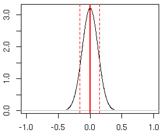
Figure 1 shows the predictive distributions of $m_{i0}$, $m_{i1}$, $m_{i2}$ and $m_{i3}$. By visual inspection, it is clear that the results of the predictive distributions of $m_{ij}$ agree with the true values used to create the dataset. In fact, the predictive distribution of $m_{i0}$ is concentrated around $0$, while the predictive distributions of $m_{i1}$, $m_{i2}$ and of $m_{i3}$ are bimodal with mode around $\{0,1\}$, $\{0,0.7\}$ and $\{0,0.4\}$, respectively.

Figure 1: Simulation scenario 1: predictive marginal distributions of $m_{i0}$(a), $m_{i1}$(b), $m_{i2}$(c) and $m_{i3}$(d) . Dashed vertical lines denote 0.05 and 0.95 posterior quantiles, while the bold vertical line indicates the posterior median.

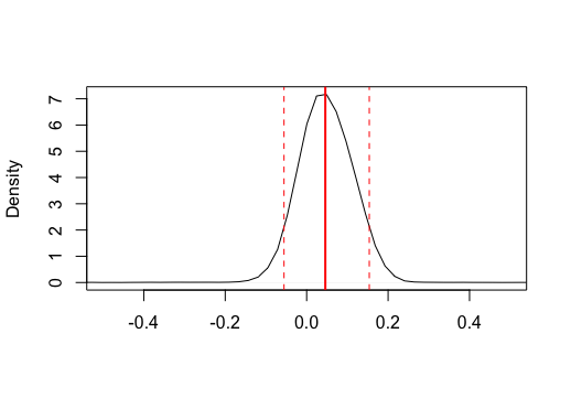
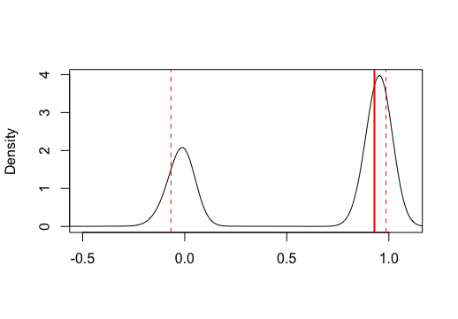
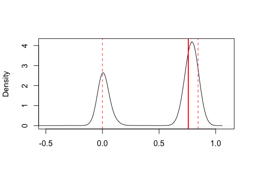
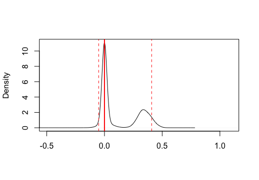
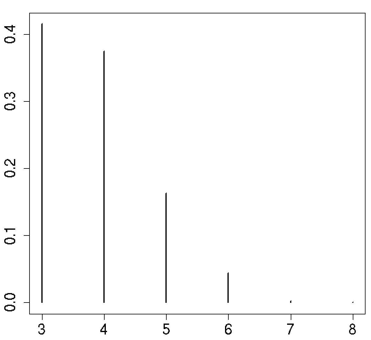
The marginal posterior distributions of $\eta_{1}$ and $\eta_{2}$, not reported here, concentrate most mass on $1$, with posterior probability of being equal to 1 of approximately 0.8 and 0.75, respectively. The marginal posterior distribution of $\eta_{3}$ shows more uncertainty, with posterior probability of being equal to 1 close to 0.44. These results capture the data generating process as 200 observations have a temporal dependency of the second order and 100 observations have a dependency of the third order. Moreover, Figure 2 displays the predictive distribution of $K$, the number of distinct components in the mixture (6)-(7). The configurations involving 3 or 4 clusters are clearly those with the highest posterior probability: posterior inference on $K$ is in agreement with the 3 components used to generate the data.

Figure 2: Simulation scenario 1: posterior distribution of $K$.

4.2 Simulation Scenario 2: Prior on the Order of Dependence

In this section we simulate a dataset of $N=200$, with $n_{i}=10$ for all $i$. Half observations are generated independently from

$$Y_{i1}\sim\mathcal{N}(0,1.5^{2}), Y_{i2}|Y_{i1}\sim\mathcal{N}(0.9\times Y_{i1},0.9^{2})$$

$$Y_{ij}|Y_{ij-1},Y_{ij-2} \sim \mathcal{N}(0.9\times Y_{ij-1}+0.7\times Y_{ij-2},0.9^{2}),\ j=3,\ldots,10$$

while the other half is independently generated from

$$Y_{i1}\sim\mathcal{N}(0,1.5^{2}), Y_{i2}|Y_{i1}\sim\mathcal{N}(-0.9\times Y_{i1},1.5^{2})$$

$$Y_{ij}|Y_{ij-1},Y_{ij-2} \sim \mathcal{N}(-0.9\times Y_{ij-1}-0.7\times Y_{ij-2},1.5^{2}),\ j=3,\ldots,10$$

As in the previous example, covariates are not present in the generating model.

We fit model (1), (10) to this dataset, with maximum order of dependence $P=3$ and prior hyperparameters (corresponding to a vague prior) set as follows:

$$\sigma_{g}^{2} = 10,\quad a_{Z}=3,\quad b_{Z}=3$$

$$\sigma \sim \mathcal{U}(0,10)$$

$$\tau \sim \mathcal{U}(0,10)$$

$$M \sim \mathcal{U}(0,5).$$

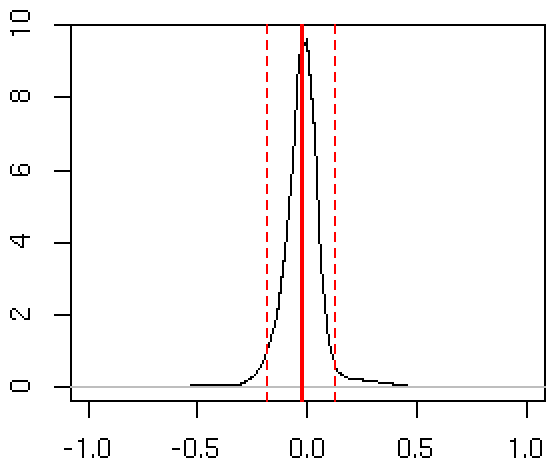
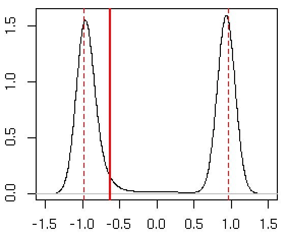
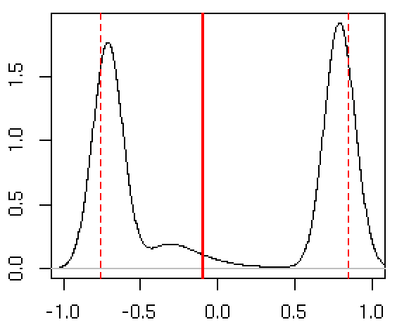
The mode of the marginal posterior distribution of $p$ is 2, with corresponding posterior probability almost 1. Conditional on $p=2$, Figure 3 reports the predictive distributions of $m_{i0}$, $m_{i1}$, $m_{i2}$ and $m_{i3}$. Once again, the result of inference are in agreement with the true parameters used to generate the data, which are realizations of a second order Markov process. From Figure 3 it is evident that the 95% posterior credible intervals (CIs) for $m_{ij}$, $j=0,1,2,3$, cover the true values. More in details, the predictive distributions of $m_{i0}$ and of $m_{i3}$ are concentrated around $0$, while the predictive distributions of $m_{i1}$ and of $m_{i2}$ are bimodal with mode around $\{-0.9,0.9\}$ and $\{-0.7,0.7\}$, respectively.

Figure 3: Simulation scenario 2: predictive marginal distributions of $m_{i0}$(a), $m_{i1}$(b), $m_{i2}$(c) and $m_{i3}$(d), conditioning on $p=2$. Dashed vertical lines denote 0.05 and 0.95 posterior quantiles, while the bold vertical line is the posterior median.

Finally, conditioning on $p=2$, the posterior mode for the number $K$ of clusters is 2, with associated posterior probability equal to 0.5.

5 Hospitalization dataset

We fit model (1)-(3) to the readmission dataset in the R package frailtypack for all the possible choices of $f$ described in Section 2.1. The dataset contains rehospitalization times (in days) after surgery in patients diagnosed with colorectal cancer. Data are available on $N=403$ patients, for a total number of $861$ recurrent events. In addition to gap times between successive rehospitalizations, the dataset contains information for each patient on the following covariates:

• chemo: variable indicating if the patient received chemotherapy.

• sex: gender of the patient.

• dukes: ordinal variable indicating the classification of the colorectal cancer. The baseline A-B denotes the invasion of the tumor through the bowel wall penetrating the muscle layer but not involving lymph nodes; the value C indicates the involvement of lymph nodes; the value D implies the presence of widespread metastases. Category D corresponds to the most severe type of cancer.

• charlson: Charlson comorbidity index. It measures ten-year mortality for a patient who may have a range of comorbidity conditions, and ranges within 3 classes, i.e. $\{0,1-2,3\}$. This is the only time-varying covariate.

The recurrent events in this study are readmission times (colorectal cancer patients may have several readmissions after first discharge). The origin of the time axis is the date of the surgical procedure for each patient and the recurrent events are next rehospitalizations related to colorectal cancer. In the analysis, we consider only patients with 6 or less events, leaving a dataset of $N=197$ patients and a total number of 495 recurrent events. Table 1 reports the number of patients with exactly $j$ gap times, for $j=1,\dots,6$. Moreover, 119 observations out of 197 are right-censored with respect to their last gap time. Since the proportion of censored data is considerably high, we need to take censoring into account.

$j$	$1$	$2$	$3$	$4$	$5$	$6$	TOT
$n_{j}$	$30$	$96$	$36$	$18$	$9$	$8$	$197$

Table 1: Number of patients for $j$ gap times, $j=1,\dots,J$.

Prior hyperparameters in (4) are set as follows:

$$\beta_{0}^{2} = 1,000$$

$$\sigma \sim \mathcal{U}(0,10)$$

$$\tau \sim \mathcal{U}(0,10)$$

$$\sigma_{g}^{2} = 10,\quad a_{Z}=3,\quad b_{Z}=3$$

$$M = 1\ .$$

5.1 Testing for the Order of Dependence

When testing the order of dependence, we first fit model (1) and (9) with $p=3$ ($G_{0}$ being a spike and slab distribution) and then model (1) and prior (10) with $P=3$.

Figure 4: Readmission dataset: predictive marginal distributions of $m_{i0}$(a), $m_{i1}$(b), $m_{i2}$(c) and $m_{i3}$(d). Dashed vertical lines denote 0.05 and 0.95 posterior quantiles, while the bold vertical line is the posterior median.

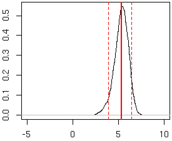
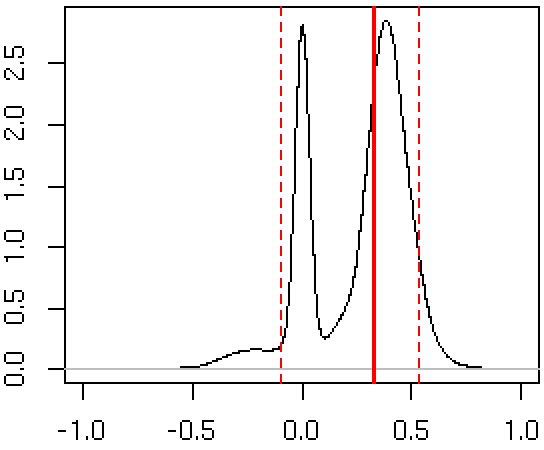
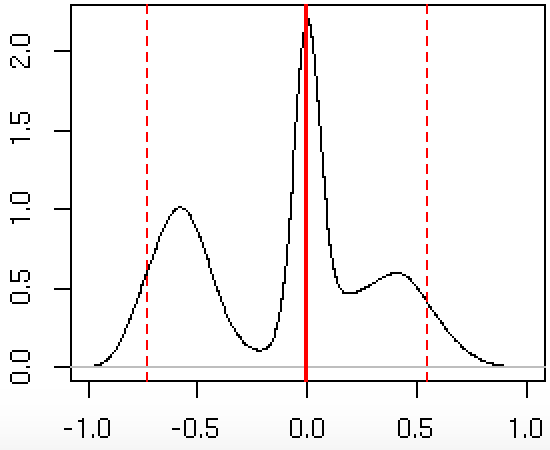
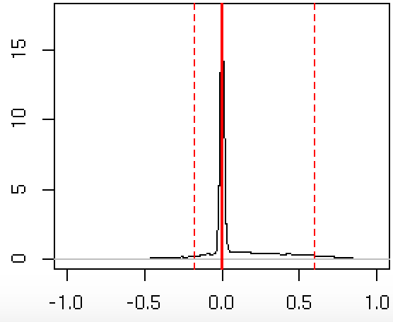
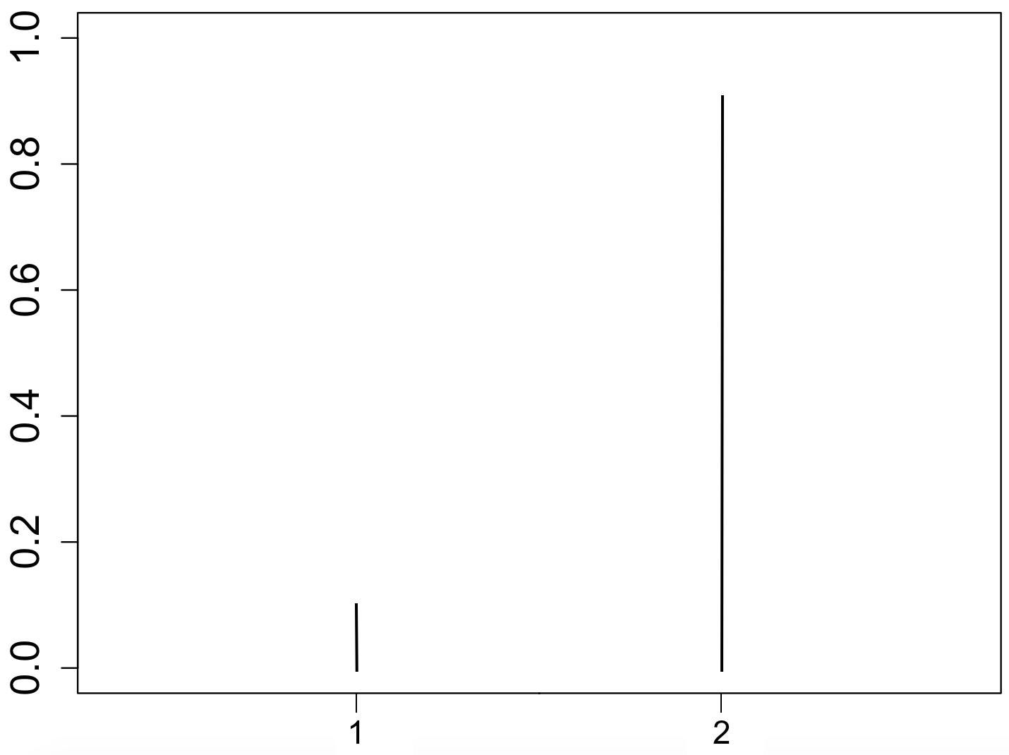
Figure 4 reports the posterior predictive marginal distributions of $m_{i,l}$, for $l=0,1,2,3$, obtained with spike and slab variable selection. Since the marginal posterior distributions of $m_{i0},m_{i1},m_{i2}$ are not concentrated around 0, unlike that of $m_{i3}$, we can conclude that the process best describing the readmission dataset has a dependency of the second order. This result is confirmed also using the approach described in Section 3.2. Indeed, the posterior distribution of $p$, displayed in Figure 5, places most of its mass on $2$.

Figure 5: Readmission dataset: posterior distribution of $p$.

5.2 Posterior analysis

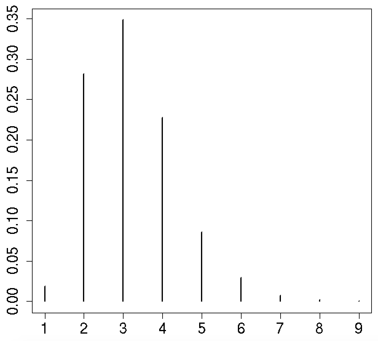
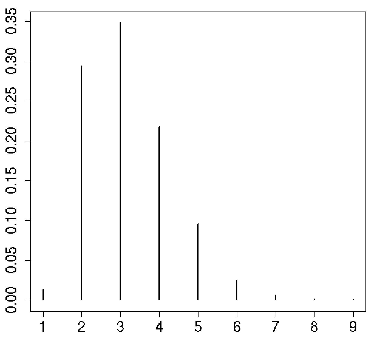
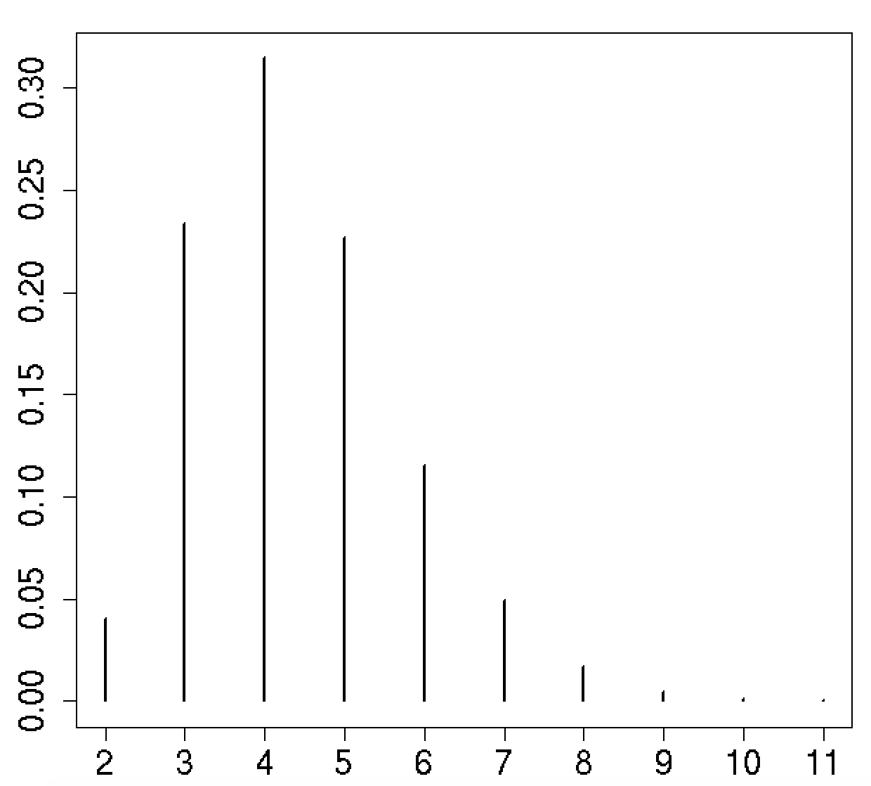
We compare now the results of the nonparametric AR(2) model for the random effects $\alpha_{ij}$’s as in (6)-(8), selected in the previous section, with models built using different choices of $f$. In particular we consider two summary statistics: $f(Y_{i1},\ldots,Y_{ij-1})=(Y_{i1}+\cdots+Y_{ij-1})/(j-1)$ and $f(Y_{i1},\ldots,Y_{ij-1})=\left(Y_{i1}\times\cdots\times Y_{ij-1}\right)^{1/(j-1)}$. The goal is to understand if higher order temporal dependency can be approximated by an AR(1)-like process built on some appropriate function of past observations as described in (2). Figure 6 displays the posterior of $K$, the number of components in the mixture (6)-(7) under different alternatives. In particular, the three plots show that the posterior modes of $K$ are 2 or 3 with a probability of around 30% for the AR(1)-type models. On the other hand, Figure 6(c), referring to the AR(2) model, suggests the existence of 3, 4 or 5 groups.

Figure 6: Readmission dataset: posterior distribution of $K$, with $f(Y_{i1},\ldots$, $Y_{ij-1})=(Y_{i1}+\cdots+Y_{ij-1})/(j-1)$ (a) and $f(Y_{i1},\ldots,Y_{ij-1})=\left(Y_{i1}\times\cdots\times Y_{ij-1}\right)^{1/(j-1)}$ (b). Panel c displays the posterior distribution of $K$ using the AR(2) model.

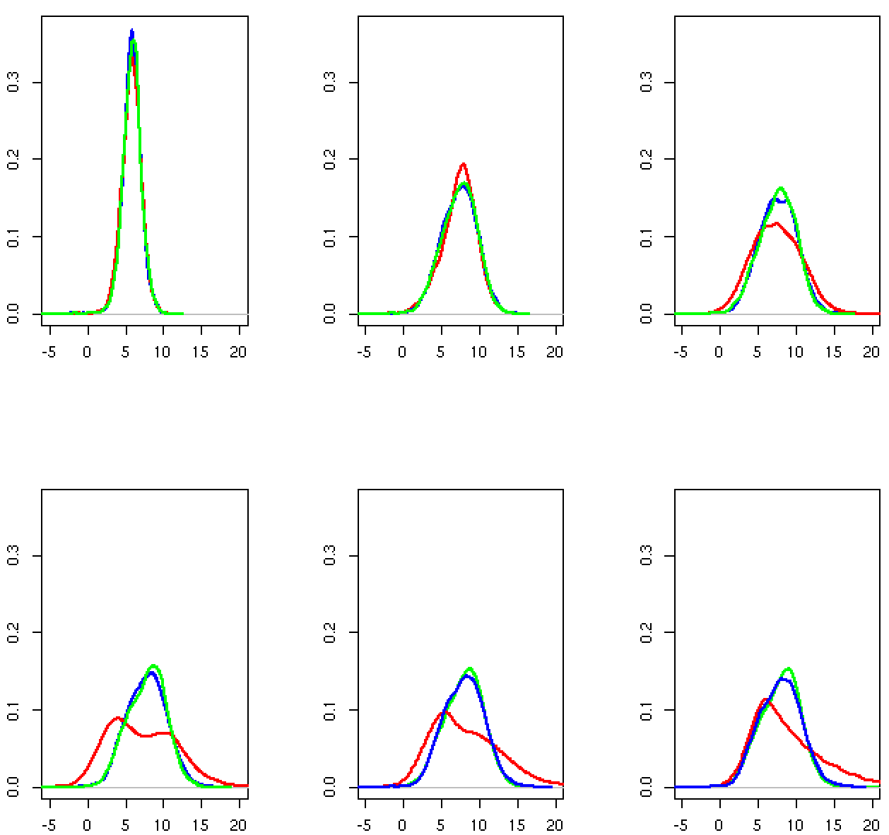
In Figure 7 we present posterior predictive distributions of $Y_{ij}$ for a hypothetical new subject, for each time $j,\ j=1,\dots,6$, setting the values of the covariates to the empirical mode. From the figure, it is evident that the two AR(1)-type models produce very similar results. Obviously, for $j=1$ and $j=2$ the three distribution are almost identical, as the models are closer. For $j>2$, it is clear that the posterior predictive distributions of $Y_{ij}$ have a larger variance and are more skewed under the AR(2) model. This experiment shows that it is not straightforward to approximate higher order dependency using summary statistics.

Figure 7: Readmission dataset: posterior predictive distributions of $Y_{ij}$, $j,\ j=1,\dots,6$.The green and blue lines represent AR(1)-type models, with $f(Y_{i1},\ldots,Y_{ij-1})=(Y_{i1}+\cdots+Y_{ij-1})/(j-1)$ and $f(Y_{i1},\ldots,Y_{ij-1})=\left(Y_{i1}\times\cdots\times Y_{ij-1}\right)^{1/(j-1)}$, respectively , and the red distribution indicates AR(2) model.

5.3 Posterior inference on the regression parameters

We now discuss the inference on the regression parameters in order to understand how covariates influence the recurrent event process. Although some covariates are fixed and do not vary over time, we still assume that their effect can be different in time and therefore we estimate a different vector of regression coefficient for all covariates in the model for each waiting time $j$, $1,\ldots,6$. Covariates chemo and sex are binary variables, while dukes and charlson are 3 levels categorical variables and we need to introduce 2 dummy variables for each of them in the model, with baseline set to A–B for dukes and to 0 for charlson. Therefore, the final covariate vector for individual $i$ is given by ${\bm{x}}_{i}=(x_{i1},x_{i2},x_{i3},x_{i4},x_{i5},x_{i6})=$(indicator for chemotherapy, indicator for female, indicator for dukes equal to C, indicator for dukes equal to D, indicator for charlson in 1 –2, indicator for charlson = 3). The vector of regression parameters ${\bm{\beta}}_{j}=(\beta_{1j},\beta_{2j},\beta_{3j},\beta_{4j},\beta_{5j},\beta_{6j})$ for each gap time $j$, $j=1,\ldots,J=6$, is therefore 6-dimensional.

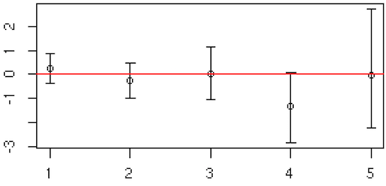
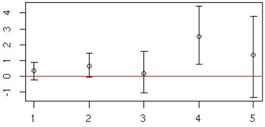
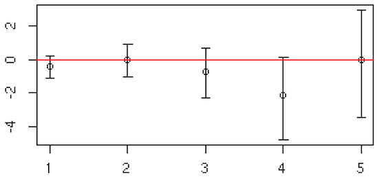
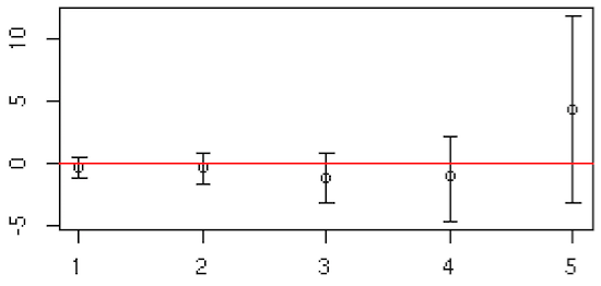
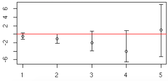
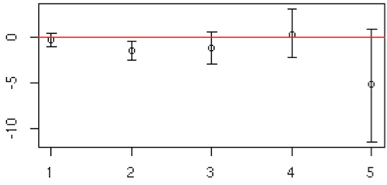
Figure 8 shows the 95% credible intervals for the posterior marginals of the regression parameters; in particular, each panel displays the posterior CIs of the regression parameter of each covariate for the first 5 gap times, i.e. of $\beta_{r1},\beta_{r2},\beta_{r3},\beta_{r4},\beta_{r5}$, where $r$ denotes the covariates. For example, Figure 8(a) shows that there is no evident effect of chemotherapy on any gap time. However, the CI of $\beta_{14}$ is concentrated on negative values, which means that chemotherapy reduces the fourth waiting time between hospitalisations. iIn general, credible intervals are larger for the last gap times, as expected, since few individuals have a large number of events. The regression coefficients at time $j=6$ are not shown as the credible intervals are not comparable with those of the previous times.

(a) Regression coefficients of chemo

(b) Regression coefficients of sex

(c) Regression coefficients of dukes = C

(d) Regression coefficients of dukes = D

(e) Regression coefficients of charlson = 1–2

(f) Regression coefficients of charlson = 3

Figure 8: Posterior 95% credible interval for the regression parameters of each covariate across the first five gap times.

6 Urinary Tract Infection dataset

We consider data on patients at risk of urinary tract infection (UTI). The best clinical marker of UTI available is pyuria, i.e. White Blood Cell count (WBC) $\mu l^{-1}$ $\geq 1$, detected by microscopy of a fresh unspun, unstained specimen of urine (Khasriya et al. (2010); Kupelian et al. (2013)). Let $T_{i0}$ correspond to the first visit attendance at the Lower Urinary Tract Service Clinic (Whittington Hospital, London, UK) and let $T_{ij}$ be the time of the $j-th$ new infection for the patient $i$. Note that at time 0, all patients suffer of UTI. For each patient and at each visit the result of the microanalysis of a sample of urine has been recorded in terms of the WBC count. Presence of WBC in the urine (regardless of the quantity) indicates the presence of Urinary Tract Infection. We include in the analysis only female patients with at least two waiting times, giving a total of $N=306$ patients. The number of observations with exactly $j$ gap times is displayed in Table 2.

j	2	3	4	5	6	7	8	9	TOT
$n_{j}$	121	89	54	21	10	6	2	3	306

Table 2: Number of observations for $j$ gap times, $j=1,\dots,9$.

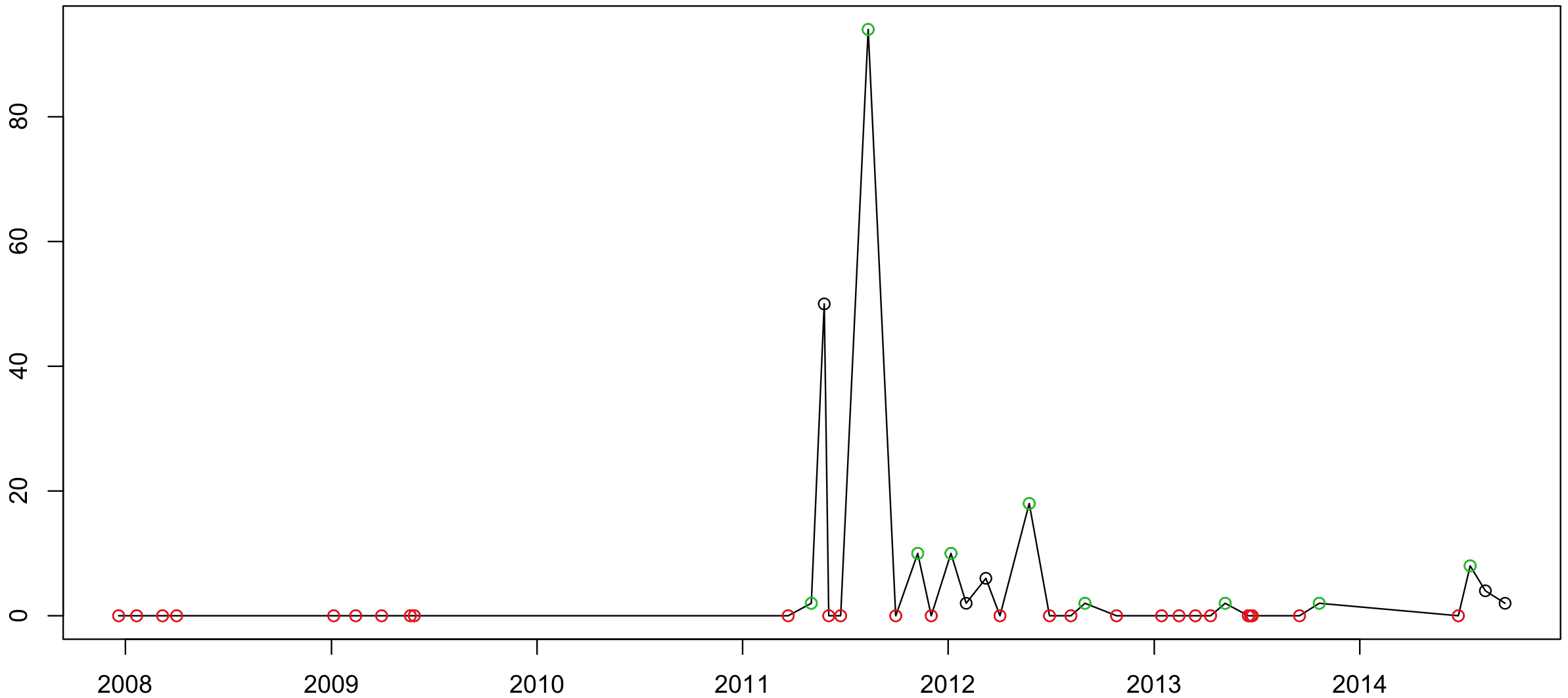
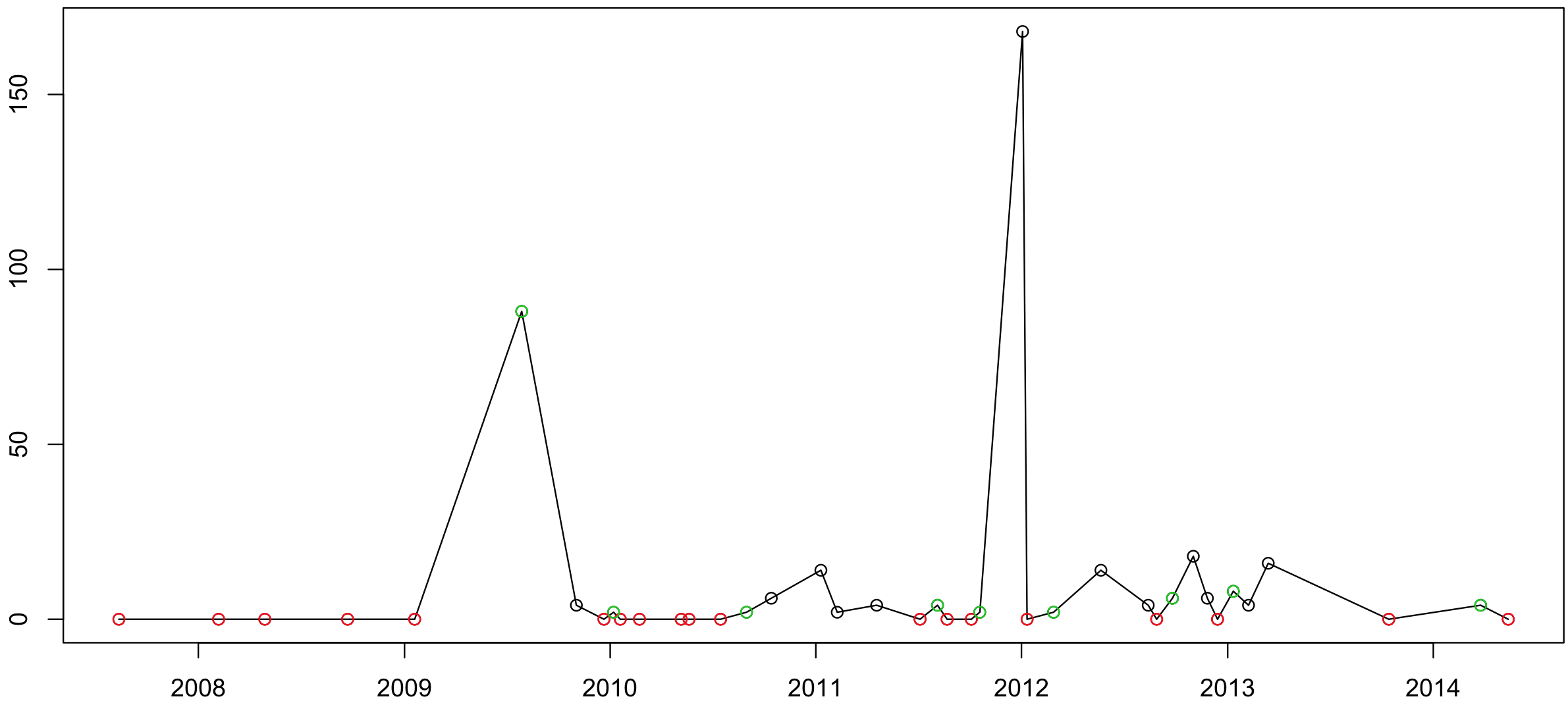
We note that 85 subjects out of 306 are right-censored with respect to their last gap time. Since the proportion of censored data is considerable, we have taken censoring into account and modified the likelihood appropriately. Figure 9 displays the recurrent events of two randomly selected patients, in which the last waiting time of the patient in the left panel is observed, while that of the patient in the right panel is censored. Indeed, the first patient suffers of infection at her last visit, while the second patient has a WBC counts equal to zero implying that a new infection will happen necessarily after her last visit.

Figure 9: Recurrent events for two patients: the last waiting time of the patient on the left is observed, while that of the patient on the right is censored. Red circles denote zero WBC at the visit while green circles denote WBC greater than 0.

We fit model (1), including for each patient a 5-dimensional vector of time-varying covariates: a continuous covariates representing the standardized age of the patient $i$ during gap time $j$ and four binary variables denoting the presence, during the $j$-th gap time, of urgency, pain, stress incontinence and voiding symptoms (=1 if the symptom is present, 0 otherwise). Therefore, the final covariate vector for individual $i$ is given by ${\bm{x}}_{i}=(x_{i1},x_{i2},x_{i3},x_{i4},x_{i5})=$(age, indicator for urgency, indicator for incontinence, indicator for pain, indicator for voiding). Descriptive statistics of the covariates are given in Table 3.

Covariate	Mean	Standard Deviation
age	53.87	16.01
presence of urgency symptoms	0.56	0.50
presence of incontinence symptoms	0.21	0.41
presence of pain symptoms	0.47	0.50
presence of voiding symptoms	0.45	0.50

Table 3: Descriptive statistics of the covariates of the UTI dataset.

In the analysis we set the prior hyperparameters in (4) in order to specify vague prior distributions:

$$\beta_{0}^{2} = 1000$$

$$\sigma \sim \mathcal{U}(0,10)$$

$$\tau \sim \mathcal{U}(0,10)$$

$$\sigma_{g}^{2} = 10,\quad a_{Z}=3,\quad b_{Z}=3.$$

$$M = 1\ .$$

6.1 Posterior Inference

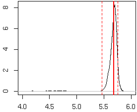
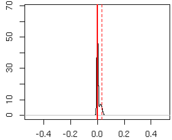
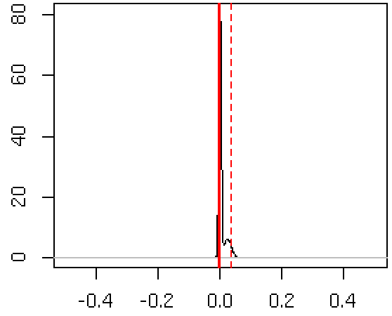
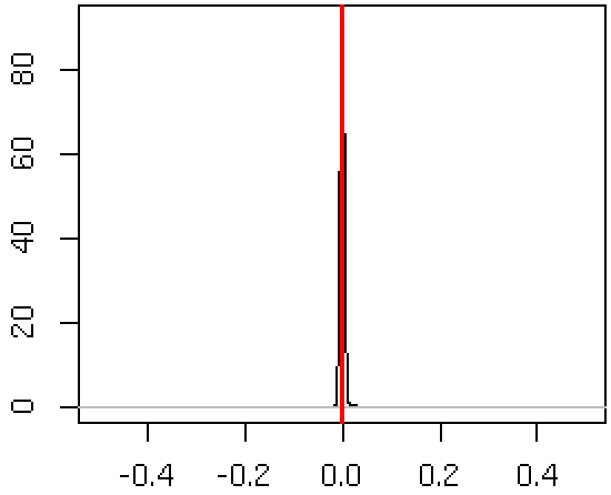
We run the model for the three choices of function $f$ described in Subsection 2.1. We obtain similar posterior predictive marginal distributions for $m_{i0}$ and $m_{i1}$, as well as the same posterior inference for $K$. In particular, a posteriori, the marginal distribution of $m_{i1}$ is concentrated around 0, indicating independence between between gap times. This result is confirmed also by performing inference on the order of dependence using both approaches introduced in Section 3. The posterior predictive marginal distributions of $m_{i,l}$, for $l=0,1,2,3$, obtained with spike and slab variable selection, is displayed in Figures 10: panel $(b)$, $(c)$ and $(d)$ show that the posterior predictive marginal distributions of $m_{i,1}$, $m_{i,2}$, $m_{i,3}$ are all concentrated around $0$. In addition, also specifying directly a prior on $p$ with $P=3$ leads to a posterior distribution for the order of temporal dependence with mode in 0 (result not shown).

Figure 10: UTI dataset: predictive marginal distributions of $m_{i0}$(a), $m_{i1}$(b), $m_{i2}$(c) and $m_{i3}$(d). Dashed vertical lines denote 0.05 and 0.95 posterior quantiles, while the bold vertical line is the posterior median.

7 Conclusion

In this work we have proposed novel Bayesian nonparametric approaches for modelling waiting times between recurrent events. Time-dependency is taken into account through the specification of an autoregressive model on the random effects governing the distributions of the gap times. To allow for clustering of patients, overdispersion and outliers, we introduce Dirichlet process mixtures as random effects distribution. Covariates may be easily included in this framework.

The strategy we adopt is flexible and allows testing for the order of dependence among random effect at different times, that is a key feature of the nonparametric AR(p) model. We propose two different methods to test the order of dependence: spike and slab variable selection and direct prior on the order of dependence. In the first case we can simply modify the base measure of the DP, whereas with the second technique, we elicit a prior on the order $p$ of the autoregressive process and then, conditioning on $p$, we set a Dirichlet Process prior of appropriate dimension for the parameters of the AR(p) model.

We can introduce the time-dependency in different ways. The simplest and probably most natural way consists of assuming that the random effects at time $j-1,\ldots,j-p$ influence the behaviour of the random effect at time $j$. We then investigate the possibility of approximating higher order of dependency using summary statistics of past observations. Our results show that the choice of summary statistics is crucial and not obvious and that the approximation worsens as the number of gap times increases. As such, this topic will of object of future research, possibly borrowing ideas from the Approximate Bayesian Computation literature.

This type of model strategy can be extended to other fields of application; in particular it is straightforward to adapt the proposed approach to model multiple time series analysis (see Nieto-Barajas and Quintana, 2016; Di Lucca et al., 2013). In fact, in this case, the data consist in $N$ time series $\mathbf{Y}_{i}=(Y_{i1},\ldots,Y_{in_{i}})$, where $i$ denotes the time series and $n_{i}$ is the number of observations for each series. The likelihood for each time series can be expressed as in (1) and temporal dependence may be introduced as in (2)-(3) with appropriate choice of the function $f(\cdot)$. Moreover, the proposed model can also be used as building block in a hierarchy to describe the relationship between recurrent events and survival up to a terminating event, for example in a survival regression context. This latter extension is object of on-going investigation.

References

- Antoniak (1974) Antoniak, C. E. (1974). “Mixtures of Dirichlet processes with applications to Bayesian nonparametric problems.” The Annals of Statistics, 2, 1152–1174.
- Clyde and George (2004) Clyde, M. and George, E. I. (2004). “Model uncertainty.” Statistical Science, 19, 81–94.
- Cook and Lawless (2007) Cook, R. J. and Lawless, J. F. (2007). The statistical analysis of recurrent events. Springer, New York.
- Di Lucca et al. (2013) Di Lucca, M. A., Guglielmi, A., Müller, P., Quintana, F. A., et al. (2013). “A simple class of bayesian nonparametric autoregression models.” Bayesian Analysis, 8, 63–88.
- Ferguson (1973) Ferguson, T. S. (1973). “A Bayesian analysis of some nonparametric problems.” The Annals of Statistics, 1, 209–230.
- George and McCullogh (1993) George, E. and McCullogh, R. (1993). “Variable selection via Gibbs sampling.” Journal of the American Statistical Association, 88, 881–889.
- George and McCulloch (1997) George, E. I. and McCulloch, R. E. (1997). “Approaches for Bayesian variable selection.” Statistica Sinica, 7, 339–373.
- Ishwaran and Zarepour (2002) Ishwaran, H. and Zarepour, M. (2002). “Exact and approximate sum representations for the Dirichlet process.” Canadian Journal of Statistics, 30, 269–283.
- Khasriya et al. (2010) Khasriya, R., Khan, S., Lunawat, R., Bishara, S., Bignal, J., Malone-Lee, M., Ishii, H., O’Connor, D., Kelsey, M., and Malone-Lee, J. (2010). “The inadequacy of urinary dipstick and microscopy as surrogate markers of urinary tract infection in urological outpatients with lower urinary tract symptoms without acute frequency and dysuria.” The Journal of Urology, 183, 1843–1847.
- Kim et al. (2009) Kim, S., Dahl, D. B., and Vannucci, M. (2009). “Spiked dirichlet process prior for bayesian multiple hypothesis testing in random effects models.” Bayesian Analysis, 4, 707–732.
- Kleinman and Ibrahim (1998) Kleinman, K. P. and Ibrahim, J. G. (1998). “A semiparametric Bayesian approach to the random effects model.” Biometrics, 54, 921–938.
- Kupelian et al. (2013) Kupelian, A. S., Horsley, H., Khasriya, R., Amussah, R. T., Badiani, R., Courtney, A. M., Chandhyoke, N. S., Riaz, U., Savlani, K., Moledina, M., Montes, S., O’Connor, D., Visavadia, R., Kelsey, M., Rohn, J. L., and Malone-Lee, J. (2013). “Discrediting microscopic pyuria and leucocyte esterase as diagnostic surrogates for infection in patients with lower urinary tract symptoms: results from a clinical and laboratory evaluation.” BJU International, 112, 231–238.
- Lo (1984) Lo, A. (1984). “On a class of Bayesian nonparametric estimates: I. Density estimates.” The Annals of Statistics, 12, 351–357.
- Müller and Rosner (1997) Müller, P. and Rosner, G. L. (1997). “A Bayesian population model with hierarchical mixture priors applied to blood count data.” Journal of the American Statistical Association, 92, 1279–1292.
- Nieto-Barajas and Quintana (2016) Nieto-Barajas, L. E. and Quintana, F. A. (2016). “A Bayesian Non-Parametric Dynamic AR Model for Multiple Time Series Analysis.” Journal of Time Series Analysis, Early View.
- Pennell and Dunson (2006) Pennell, M. L. and Dunson, D. B. (2006). “Bayesian semiparametric dynamic frailty models for multiple event time data.” Biometrics, 62, 1044–1052.
- Plummer (2003) Plummer, M. (2003). “JAGS: A program for analysis of Bayesian graphical models using Gibbs sampling.”
- Plummer et al. (2006) Plummer, M., Best, N., Cowles, K., and Vines, K. (2006). “CODA: Convergence Diagnosis and Output Analysis for MCMC.” R News, 6, 7–11.
- Quintana and Müller (2012) Quintana, F. A. and Müller, P. (2012). “Nonparametric Bayesian assessment of the order of dependence for binary sequences.” Journal of Computational and Graphical Statistics, 13, 213–231.
- Sethuraman (1994) Sethuraman, J. (1994). “A constructive definition of Dirichlet priors.” Statistica Sinica, 4, 639–650.