Propagation of gravitational waves in an expanding background in the presence of a point mass

Abstract

We solve the Laplace equation $\Box h_{ij}=0$ describing the propagation of gravitational waves in an expanding background metric with a power law scale factor in the presence of a point mass in the weak field approximation (Newtonian McVittie background). We use boundary conditions at large distances from the mass corresponding to a standing spherical gravitational wave in an expanding background which is equivalent to a linear combination of an incoming and an outgoing propagating gravitational wave. We compare the solution with the corresponding solution in the absence of the point mass and show that the point mass increases the amplitude of the wave and also decreases its frequency (as observed by an observer at infinity) in accordance with gravitational time delay.

I Introduction

The theoretical prediction of gravitational waves (GWs) originates in 1893 when Heaviside first discussed the possibility of their existence. In 1916 Einstein predicted their existence Einstein (1916, 1918) in the context of general relativity. In the linearized weak-field approximation, he found that his equations had transverse wave solutions travelling at the speed of light Ellis et al. (2016) produced by the time dependence of the mass quadrupole moment of the source Le Tiec and Novak (2016). Einstein realized that GW amplitudes would be small and up until 1957, there was debate about the physical relevance of their existence Saulson (2011).

Nevertheless, the discovery of the binary pulsar system PSR B1913+16 by Hulse and Taylor Hulse and Taylor (1975) and subsequent observations of its energy loss by Taylor and Weisberg Taylor and Weisberg (1982) demonstrated indirectly the existence of GWs. This discovery, along with subsequent related analysis Press and Thorne (1972), led to the recognition that a possible direct detection and analysis of GWs could reveal interesting properties of various relativistic systems and could also provide new tests of general relativity, especially in the strong-field regime.

Recently, Abbot et al Abbott et al. (2016a, b), reported the first direct detection of GWs emitted by a binary black hole (BBH) system merging to form a single black hole (BH). Their observation provides a direct window to the properties of space time in the strong-field limit and is consistent with predictions of general relativity for the nonlinear dynamics of highly disturbed BHs. The announced beautiful discovery is the result of great efforts for a century by several scientists Abbott et al. (2016b) (and references therein). It is a great investigation, because we have now one more window to the Universe and one more confirmation of the theory of general relativity. Such GW observations can be used to test the equivalence principle Kahya and Desai (2016); Wu et al. (2016); Liu et al. (2016); Yunes et al. (2016), test the propagation of GWs Yunes et al. (2016); Branchina and De Domenico (2016); Schreck (2016); Arzano and Calcagni (2016); Bicudo (2016); Collett and Bacon (2016); Blas et al. (2016); García-Bellido et al. (2016), test the validity of general relativity Konoplya and Zhidenko (2016); Moffat (2016); Vainio and Vilja (2016), constrain early cosmological phase transitions Dev and Mazumdar (2016); Jaeckel et al. (2016), probe the quantum structure of black holes Giddings (2016) or the connection between dark matter and primordial black holes Sasaki et al. (2016); Bird et al. (2016); Clesse and García-Bellido (2016).

The recent direct discovery of the GWs has been achieved by the LIGO/Virgo collaboration associating the GW 150914 event Abbott et al. (2016a, b); Maselli et al. (2016) to the coalescence of a BBH. This binary detection suggests that BBH masses and merging rates may be higher than estimated previously. The rates however, are in agreement with more recent estimates, obtained with a population synthesis approach, predicting the early formation of detectable BBH Dominik et al. (2012, 2015). Thus, the stochastic gravitational waves background (SGWB) produced by merging cosmological BBH sources could be larger than previously assumed Maselli et al. (2016) (and references therein) and may be detectable by advanced detectors Abbott et al. (2016c).

A stochastic background of relic gravitational waves (RGWs) is predicted by inflationary models Nakama and Suyama (2015, 2016) and has been well studied Starobinsky (1979); Abbott and Harari (1986). The power spectrum of relic gravitational wave background reflects the physical conditions in the early Universe thus providing valuable information for cosmology Dufaux et al. (2007). This spectrum is determined by the early stage of inflation as well as by the expansion properties of the subsequent epochs, including the current one. The calculation of the spectrum Allen (1988); Henriques (2004) was initially performed for a currently decelerating universe. However, it is now well known that the universe expansion is currently accelerating Riess et al. (1998); Perlmutter et al. (1999) and since the evolution of RGWs depends on the expanding background space time, the spectrum of RGWs should be modified accordingly. This modification was confirmed and studied in Refs Zhang et al. (2005); Izquierdo and Pavon (2004) using the well-known formulation of GWs in an expanding Universe Grishchuk (1975) and an approximation of the scale factor $a(\tau)$ in the context of a sequence of successive expansion epochs, including the current stage of accelerating expansion. It was found that the current accelerating expansion induces modifications in both the shape and the amplitude of the RGW spectrum.

Since existence of RGWs is a key prediction of the inflationary models, their detection could provide evidence that inflation actually took place. Thus, it is important to accurately calculate the expected detailed form of the RGW spectrum. Calculations related to RGWs in an accelerating Universe have been performed Zhao (2007) and a numerical method has been developed to calculate the power spectrum of the RGWs. Late evolution of RGWs in coupled dark energy models has been examined extensively in Ref. Sosa Almazan and Izquierdo (2014).

Even though the effects of cosmological expansion on GWs have been investigated mainly in the context of RGWs, these effects are relevant in all cases when the source is located at cosmologically large distances from the observer (redshift $z\geq 0.1$). The GW 150914 ($z=0.09$) event is in the limit of such distances and therefore, the effects of cosmic expansion may be relevant. Thus a wide range of studies have investigated the effects of cosmological expansion of GWs from a variety of viewpoints including the effects of expansion on the GW group and phase velocities Balek and Polak (2009); L.Brillouin (1960), mathematical aspects and exact solutions Fabris and de Borba Goncalves (1998); Alekseev and Griffiths (1995); Tauber (1984); Waylen (1978); Tamayo et al. (2015), quantum and thermodynamic properties of GWs Arzano and Calcagni (2016),Izquierdo Saez (2005), general properties Hartnett and Tobar (2008); Waylen (1978); Jackson (1972) nonlinear effects Ikeda et al. (2015), properties of the GW energy momentum tensor Su and Zhang (2012), collision of GWs with electromagnetic waves Alekseev (2016), evolution of GWs in gravitational plasma Baptista and Gerbal (1982) etc .

Even though these studies have properly taken into account the expansion of the background metric, they have not taken into account the effects of the gravitational field of mass distributions on the evolution of the GWs. Such a gravitational field combined with the expanding background may induce new observable effects on the spectrum of propagating gravitational waves affecting the amplitude and the frequency of such waves (due to gravitational time delay) Zeldovich (1992).

Assuming spherical symmetry, the background metric around a point mass embedded in an expanding Friedmann-Lemaitre-Robertson-Walker(FLRW) cosmological background is well approximated by the McVittie McVittie (1933); Stephani et al. (2003) spacetime. Such a metric is further simplified in the Newtonian limit and has been used as the background metric for the investigation of bound system geodesics in phantom and quintessence cosmologies Nesseris and Perivolaropoulos (2004a); Antoniou and Perivolaropoulos (2016); Faraoni and Jacques (2007); Nolan (2014). This metric can also be used as a background for the propagation of GWs in order to investigate the influence of a mass distribution of a GW propagating in an expanding cosmological background.

In the present analysis we address the following question: ’What are the weak field effects of a point mass on a multipole spherical wave component of a GW evolving in an expanding background in the vicinity of the mass?’. In particular we numerically solve the dynamical equation for the evolution of GWs in the background of the Newtonian McVittie metric and identify the effects induced by the point mass on the amplitude and frequency of the evolving GW as a function of the parameters determining the mass for fixed background expansion rate. As a test of our analysis, in the zero mass limit, our numerical solution reduces to the well known analytic solution of a GW evolving in an expanding background.

The structure of this paper is the following: In the next section we review the wave equation and the behavior of the GW in a homogeneous-isotropic expanding background. We also derive the gravitational wave equation in a background metric corresponding to the Newtonian limit of the McVittie metric. In section $III$ we solve numerically the wave equation in the Newtonian McVittie background and identify the new features induced in the GW by the presence of the point mass. Finally in section $IV$ we conclude, summarize and discuss possible extensions on this analysis.

II Gravitational Waves in Expanding Universe in the Presence of Point Mass

We first briefly review the propagation evolution of a plane GW in the $\hat{z}$ direction (the direction of the wavevector $\vec{k}$) with tensor perturbations in the $x-y$ plane. The perturbations to the metric are described by two functions, $h_{+}$ and $h_{\times}$, assumed small. We use the FRW metric in cartesian coordinates with the components $g_{00}=1$, zero space-time components $g_{0i}=0$, and set $c=1$. The spatial part of the metric is of the form:

$$g_{ij}=-a^{2}(t)\begin{pmatrix}1+h_{+}&h_{\times}&0\\ h_{\times}&1-h_{+}&0\\ 0&0&1\\ \end{pmatrix}$$ (1)

The perturbation tensor $H_{ij}$ is symmetric, divergenceless, traceless and has the form:

$$H_{ij}=\begin{pmatrix}h_{+}&h_{\times}&0\\ h_{\times}&-h_{+}&0\\ 0&0&1\\ \end{pmatrix}$$ (2)

From the Einstein equations for tensor perturbations, it is easy to derive a set of equations governing the evolution of the tensor variables $h_{+}$ and $h_{\times}$. We write the FRW metric in cartesian coordinates and in conformal time $\tau$ (defined by $dt=ad\tau$), in the form

$$ds^{2}=a^{2}(\tau)[d\tau^{2}-(\delta_{ij}+H_{ij})dx^{i}dx^{j}]$$ (3)

The dynamical equation determining the evolution of the GWs is of the form:

$$\Box H_{ij}=\partial_{\mu}(\sqrt{-g}\partial^{\mu}H_{ij}(\vec{r},\tau))=0$$ (4)

Since all components of the tensor perturbations evolve in accordance with the same wave equation (4) we may set $H_{k}\equiv H_{ij}$. Without loss of generality we assume propagation in the $z$ direction and thus we use the ansatz:

$$H_{k}(\tau,z)=h_{k}(\tau)e^{\pm ikz}$$ (5)

Using eq. (5) in (4) we find the dynamical equation for the evolution of gravitational waves in conformal time in an FRW background as

$$h^{\prime\prime}_{k}+2\frac{a^{\prime}}{a}h^{\prime}_{k}+k^{2}h_{k}=0$$ (6)

where the prime ^′ denotes the derivative with respect to conformal time. Notice that all of the perturbation tensor components obey the same equation. We introduce a rescaling of conformal time as $\bar{\tau}=k\tau$ and thus it becomes clear that

$$h_{k}(\tau)=h(k\tau)$$ (7)

The rescaling expressed by eq. (7) can only be made in conformal time provided that the scale factor is a power law $a(\tau)\sim\tau^{\alpha}$. In the radiation dominated epoch we have $\alpha=1$ and during the matter dominated era $\alpha=2$. The wave solution (5) can be written in spherical coordinates as:

$$H_{k}(\tau,\rho,\theta)=h(k\tau)e^{\pm ik\rho\cos\theta}$$ (8)

The spectrum of the GWs may be obtained as  Zhang et al. (2006):

$$P(k,\tau)=\frac{4\;l_{Pl}}{\sqrt{\pi}}k\mid h(k\tau)\mid$$ (9)

where $l_{Pl}\sim\sqrt{G}$ is the Planck length. The plane wave of equation (8) can be expanded in spherical waves as:

$$e^{ik\rho\cos{\theta}}=\sum_{l=0}^{\infty}i^{l}(2l+1)j_{l}(k\rho)P_{l}(\cos{\theta})$$ (10)

where $j_{l}(x)$ are the spherical Bessel functions and $P_{l}(\cos{\theta})$ are Legendre’s polynomials. Thus, the partial spherical GW is (at order $l$)

$$H_{ij}(\tau,\rho,\theta)\sim h(k\tau)j_{l}(k\rho)P_{l}(\cos{\theta})$$ (11)

After rescaling, the dynamical equation (6) is written as:

$$h^{\prime\prime}(k\tau)+2\frac{a^{\prime}}{a}h^{\prime}(k\tau)+h(k\tau)=0$$ (12)

where the prime ^′ now denotes differentiation with respect to the rescaled conformal time $k\tau$.

Assuming a power law for the background scale factor as $a(\tau)\sim\tau^{\alpha}$, the solution of the wave equation (12) can be written in terms of incoming and outgoing waves (Hankel functions) as

$$h(k\tau)=\frac{1}{a(\tau)}(\tilde{A}_{k}\sqrt{k\tau}H^{(1)}_{\alpha-1/2}(k\tau)+\tilde{B}_{k}\sqrt{k\tau}H^{(2)}_{\alpha-1/2}(k\tau))$$ (13)

where $H^{(1)}$, $H^{(2)}$ are the Hankel functions and $\tilde{A}_{k}$, $\tilde{B}_{k}$ are arbitrary constants which may depend on $k$ and are determined by the initial conditions. This solution may also be written in terms of standing waves as

$$h(k\tau)=(k\tau)^{\frac{1}{2}-\alpha}(A_{k}J_{\alpha-1/2}(k\tau)+B_{k}Y_{\alpha-1/2}(k\tau))$$ (14)

where $J$,$Y$ are the Bessel functions of first and second kind respectively and $A_{k}=\tilde{A}_{k}k^{\alpha}$, $B_{k}=\tilde{B}_{k}k^{\alpha}$. Thus, for a power law scale factor the spherical GW is

$$H_{k}(\tau,\rho,\theta)=(k\tau)^{\frac{1}{2}-\alpha}(A_{k}J_{\alpha-1/2}(k\tau)+B_{k}Y_{\alpha-1/2}(k\tau))$$

$$j_{l}(k\rho)P_{l}(cos\theta)$$ (15)

As a warm up exercise before the introduction of a point mass in the metric, we now rederive the solution (14), (15) starting from the FRW metric in spherical coordinates

$$ds^{2}=a(\tau)^{2}\{d\tau^{2}-[d\rho^{2}+\rho^{2}(d\theta^{2}+\sin^{2}{\theta}d\phi^{2})]\}$$ (16)

Because of the azimuthal symmetry, the solution doesn’t depend on the variable $\phi$ we will seek solutions of the Eq. (4) of the form

$$H_{k}(\tau,\rho,\theta,\phi)=f(\tau)R(\rho)P_{l}(cos\theta)$$ (17)

From the Eqs. (4),(17), after separation of variables we find

$$\frac{1}{R}[\frac{d^{2}R}{d\rho^{2}}+\frac{2}{\rho}\frac{dR}{d\rho}-\frac{l(l+1)}{\rho^{2}}]=-k^{2}$$ (18)

and

$$\frac{1}{f}[\frac{d^{2}f}{d\tau^{2}}+\frac{2a^{\prime}}{a}\frac{df}{d\tau}]=-k^{2}$$ (19)

where $k^{2}$ is arbitrary constant. As expected eq. (19) is identical to eq. (6) while eq. (18) is the spherical Bessel equation with acceptable solution

$$R_{l}(\rho)=A_{l}j_{l}(k\rho)$$ (20)

We thus reobtain the general solution in spherical coordinates (15).

We can now generalize the above analysis to investigate the behavior of GWs when they interact with a point mass $M$. In the presence of a point mass and cosmological expansion, the appropriate background metric is the McVittie metric. In the Newtonian limit, using comoving coordinates the McVittie metric is Antoniou and Perivolaropoulos (2016); Nesseris and Perivolaropoulos (2004b):

$$ds^{2}=(1-\frac{R_{s}}{\rho a(t)})dt^{2}-a(t)^{2}[d\rho^{2}+\rho^{2}(d\theta^{2}+\sin^{2}{\theta}d\phi^{2})]$$ (21)

where $R_{s}=2GM$. The angular variable $\theta$ separates and thus we use the perturbation ansatz

$$H_{k}(t,\rho,\theta,\phi)=Q(t,\rho)P_{l}(cos\theta)$$ (22)

$\begin{array}[]{@{\hspace{-0.10in}}c@{\hspace{0.0in}}c}\lx@intercol\mbox{}\hfil\lx@intercol&\lx@intercol\mbox{}\hfil\lx@intercol\\[-14.45377pt] \epsfbox{fig0a.eps}\hfil&\epsfbox{fig0b.eps}\hfil\\ \end{array}$

Figure 1: a: A superposition of the analytic solution with the numerical simulation initial condition taken at $\tau=1$. The spherical wave with $l=6$ and scale factor $a(\tau)=\tau$ is shown. b: The numerically evolved solution (dashed red line) for the gravitational wave $Q(\tau,\rho)$ at $\tau=16.5$ with $R_{s}=0$, is in excellent agreement with the corresponding analytic evolved solution (blue line). This is a test of the quality of the numerical solution.

Using the background metric (21) and the ansatz (22) in the gravitational wave equation (4) we obtain the dynamical equation for $Q(t,\rho)$ as

$$\frac{\partial^{2}Q}{\partial\rho^{2}}+\frac{2}{\rho}(1-\frac{3R_{s}}{4a\rho})(1-\frac{R_{s}}{a\rho})^{-1}\frac{\partial Q}{\partial\rho}-\frac{l(l+1)Q}{\rho^{2}}=$$

$$\frac{a^{2}}{1-\frac{R_{s}}{a\rho}}[\frac{\partial^{2}Q}{\partial t^{2}}+\frac{3\dot{a}}{a}(1-\frac{7R_{s}}{6a\rho})(1-\frac{R_{s}}{a\rho})^{-1}\frac{\partial Q}{\partial t}]$$ (23)

Assuming that

$$\frac{R_{s}}{a\rho}\ll 1$$ (24)

and keeping terms $R_{s}/a\rho$ only in first order we can write eq. (II) in conformal time as

$$(1+\frac{R_{s}}{a\rho})\frac{\partial^{2}Q}{\partial\tau^{2}}+\frac{2a^{\prime}}{a}(1+\frac{3R_{s}}{4a\rho})\frac{\partial Q}{\partial\tau}$$

$$=\frac{\partial^{2}Q}{\partial\rho^{2}}+\frac{2}{\rho}(1+\frac{R_{s}}{4a\rho})\frac{\partial Q}{\partial\rho}-\frac{l(l+1)Q}{\rho^{2}}$$ (25)

Eq. (II) is not separable and it is not tractable analytically in a simple manner. As expected, in the limit of zero mass it separates and reduces to eqs. (18) and (19).

In the next section we integrate eq. (II) numerically and investigate the dependence of the solution on the values of the parameter $R_{s}$. It will be seen that as the wave approaches the point mass it experiences two types of distortion

• gravitational time delay and increase of its period in conformal cosmological time.

• Its amplitude increases in comparison to the amplitude it would have in the absence of the point mass.

According to general relativity the expected period of the wave at a comoving distance $\rho$ from the point mass, as measured by an observer at infinity, is

$$T=\frac{T_{0}}{\sqrt{1-\frac{R_{s}}{a\rho}}}$$ (26)

where $T_{0}$ is the corresponding period at infinity (or in the absence of the mass). For small mass or large distance from the source the increase of the period is

$$\frac{\Delta T}{T_{0}}=\frac{1}{2a\rho}R_{s}$$ (27)

where $\Delta T=T-T_{0}$ is the difference of the wave periods with and without the presence of the mass. The validity of eq. (27) for the GW in the vicinity of a point mass will be demonstrated numerically in the next section.

III Numerical Analysis

In order to keep the analogy with the massless case $R_{s}=0$ we rescale the dynamical equation (II) to dimensionless form using the wavenumber $k$ defining $k\rho=\bar{\rho}$, $k\tau=\bar{\tau}$. In this case we have an additional physical dimensionless parameter:

$$\bar{R_{s}}=kR_{s}$$ (28)

In the numerical analysis that follows we only use dimensionless quantities even though we will omit the bar in what follows.

$\begin{array}[]{@{\hspace{-0.10in}}c@{\hspace{0.0in}}c}\lx@intercol\mbox{}\hfil\lx@intercol&\lx@intercol\mbox{}\hfil\lx@intercol\\[-14.45377pt] \epsfbox{fig1a.eps}\hfil&\epsfbox{fig1b.eps}\hfil\\ \epsfbox{fig1c.eps}\hfil&\epsfbox{fig1d.eps}\hfil\end{array}$

Figure 2: The evolution of the profile of a partial spherical gravitational wave with $l=6$, $R_{s}=5$ (red dashed line) in comparison with the corresponding free solution ($R_{s}=0$, blue continuous line). The free wave reaches its maximum first (Fig. 1b) while the wave in the presence of the point mass shows a delay in reaching its maximum (Fig. 1c) due to gravitational redshift. The wave in the presence of the mass has a higher amplitude (compare 1b with 1c) in the vicinity of the mass and the phase difference increases with time in the vicinity of the mass (Fig. 1d).

We solve numerically eq. (II) with initial conditions corresponding to a standing gravitational wave evolving in a homogeneous FRW spacetime ($R_{s}=0$) using eq. (14) with $B_{k}=0$ starting the evolution at $\tau=1$. This is equivalent to assuming that the point mass appears at $\tau=1$. For definiteness we set $\alpha=1$ or $a(\tau)\sim\tau$ corresponding to an expanding background in the radiation era. The boundary conditions are imposed for $Q$ and for its first derivative at large $\rho$ where the effects of the point mass are negligible and also correspond to a standing GW evolving in a homogeneous FRW spacetime ($R_{s}=0$) using eq. (14) with $B_{k}=0$.

The Bessel function boundary condition (14)-(15) we have used for the wave equation at large distance from the source, describes a standing GW which however can be expressed as a superposition of two propagating modes (Hankel functions). The asymptotic behaviour of Hankel functions, which is proportional to $e^{i\tau}$, corresponds to a propagating GW, while the asymptotic behavior of Bessel functions is proportional to $\cos(\tau)$ and corresponds to a standing GW.

We stress that since we have made the Newtonian approximation our results are reliable in regions where the weak field condition (24) is satisfied.

We thus construct numerically the solution $Q(\rho,\tau,R_{s},l,\alpha)$ and compare with the corresponding analytical solution $Q(\rho,\tau,R_{s}=0,l,\alpha)$. We have tested our numerical evolution by verifying that the numerical solution for $R_{s}=0$ agrees with the corresponding analytical solution at a level better that $1\%$ (Fig. 1).

Following the above comments about the boundary condition we fix $Q$ (and its derivative) at the boundary $\rho_{end}>500$ using eq. (15) with $\alpha=1$, $A_{k}=1$ and $B_{k}=0$ as

$$Q(\tau,\rho_{bound})=\sqrt{\frac{2}{\pi}}\frac{\sin(\tau)}{\tau}j_{l}(\rho_{bound})$$ (29)

Similarly, the initial conditions set at $\tau_{i}=1$ are:

$$Q(\tau_{i},\rho)=\sqrt{\frac{2}{\pi}}\frac{\sin(\tau_{i})}{\tau_{i}}j_{l}(\rho)$$ (30)

and

$$\frac{\partial Q(\tau_{i},\rho)}{\partial\tau}=\frac{\partial}{\partial\tau}[\sqrt{\frac{2}{\pi}}\frac{\sin(\tau)}{\tau}j_{l}(\rho)]|_{\tau=\tau_{i}}$$ (31)

In addition to the test of the validity of numerical solution presented in Fig. 1 we have performed other tests including the verification of the independence of the numerical solution from the location of the boundary for $\rho_{bound}>200$.

We have solved the partial differential equation (II) for various values of $l$ with results that are qualitatively similar. For definiteness we present in Fig. 2 the solution corresponding to $l=6$ for $R_{s}=5$ superposed with the corresponding solution for $R_{s}=0$ in order to identify the new features introduced in the evolution of the GW by the presence of the point mass.

There are three main features to observe in Fig. 2. First, the waves are practically identical far away from the point mass as expected. Second, there is a time delay for the wave in the presence and in the vicinity of the point mass (Fig. 2b upper right). Third, the amplitude of the wave in the presence and in the vicinity of the mass increases (compare Fig. 2b (upper right) with Fig. 2c (lower left)).

The main effect of the expansion is to reduce the amplitude of the gravitational wave by a factor proportional to the scale factor in the absence of the mass. This is shown in Fig. 3 which shows that the amplitude multiplied by the scale factor remains constant in the absence of the mass (blue oscillating line has constant amplitude) for the particular time dependence of the scale factor considered ($a(\tau)\sim\tau$). In the presence of the mass however, the decrease of the amplitude due to the expansion is less efficient (red line) and the product of the amplitude times the scale factor increases slowly with time.

The gravitational wave time evolution shown in Fig. 3 corresponds to $\rho=7.9$ (closest maximum amplitude to the mass for $l=6$) for $R_{s}=5$ (red dashed line) and is superposed with the corresponding evolution for $R_{s}=0$ (blue continuous line). This plot demonstrates the relative (linear) increase of the amplitude with time, as well as the increased period of the wave in the presence of the mass. It also demonstrates (as discussed above) the well known fact that the wave amplitude in the absence of the mass ($R_{s}=0$) is inversely proportional to the scale factor (the blue wave has a constant amplitude).

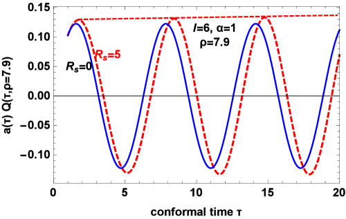
Figure 3: The time evolution of the first spatial maximum (at $\rho=7.9$) of the partial spherical wave with $l=6$, $R_{s}=5$ (red line) in comparison with the corresponding free solution ($R_{s}=0$, blue continuous line) at the same spatial point. The free wave reaches its maximum first (Fig. 2b) while the wave in the presence of the point mass shows a delay in reaching its maximum (Fig. 2c) due to gravitational redshift. The wave in the presence of the mass has an amplitude that increases with time as indicated with the dashed red line that in tangent to the gravitational wave maxima. As expected, the product $a(\tau)Q(\tau)$ is constant for the free wave in an expanding background.

The effects of the gravitational time delay on the evolution of the wave may also be demonstrated by plotting the power spectrum obtained by a Fourier series expansion of the evolving in conformal time numerical solution at $\rho=7.9$ in harmonic waves.

The finite time interval power spectrum may be defined through the expansion

$$Q(\tau,\rho)=\frac{a_{0}}{2}+\sum\limits_{i=1}^{n}(a_{n}\cos(n\tau)+b_{n}\sin(n\tau))$$ (32)

as

$$P(n)\equiv\log\sqrt{a_{n}^{2}+b_{n}^{2}}$$ (33)

We used a time interval of approximately two complete oscillations which corresponds to a time interval $\tau\in[1,20]$ ($\tau_{i}=1,\tau_{max}=20$ as shown in Fig. 4).

As shown in Fig. 4 the presence of the mass (red continuous line) leads to an increase of the amplitude of low harmonics and decrease of the amplitude of higher harmonics which is consistent with the effects of gravitational time delay. The exact form of the spectrum clearly depends on the time interval considered, however the qualitative feature of higher amplitudes for lower frequencies persists for all time intervals. This feature is more prominent for lower values of $\rho$.

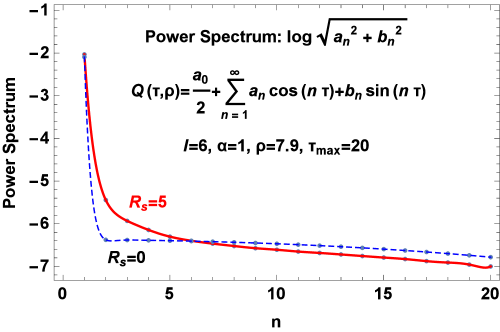
Figure 4: The time power spectra of the gravitational wave in the presence (red line) and in the absence (blue line) of the mass. Notice that lower frequencies have a higher amplitude for the wave in the presence of the mass as expected due to the gravitational time delay.

In accordance with eq. (27) the increase of the period of the wave at a given distance from the mass is proportional to the mass in the weak field approximation. This is consistent with our numerical solution as shown in Fig. 5 where we show the relative increase of the period of the wave $\Delta T/T_{0}$ at given distances $\rho$ from the mass ($\rho=7.9$ and $\rho=15.89$) for various values the parameter $R_{s}$ (points in plot). In order to evaluate the relative change of the period $\Delta T/T_{0}$ we use the time evolution of the wave perturbation as shown in Fig. 3 to obtain the period of the wave in the presence of the mass and the corresponding period in the absence of the mass. Superposed in Fig. 5 is the best fit straight line in each case. As is theoretically expected there is a linear relationship in accordance with eq. (27). The correlation coefficients of the points with the corresponding best fit straight line are equal to $0.99$ indicating an excellent quality of fit.

The theoretically predicted slope is $\frac{1}{2a\rho}$ where the scale factor can be taken as approximately constant and equal to its average value during the wave period used to evaluate $\Delta T/T_{0}$.

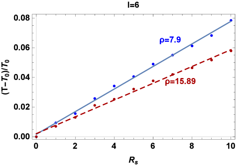
Figure 5: The relative difference of the wave periods $\Delta T/T_{0}$, where $T$ is the period in the presence of mass and $T_{0}$ is the period in the absence of mass, as a function of $R_{s}$. It is clear that as the value of the variable $\rho$ increases, the statistical slope of the curve decreases. This is an anticipated result due to theoretical slope of the curve $\frac{1}{2a\rho}$.

In order to estimate the theoretical value of the scale factor, we calculate the mean value $\bar{a}(\tau)$, in the time interval $\tau_{1}-\tau_{2}$ of a single period, through the formula:

$$\bar{a}(\tau)=\frac{1}{\tau_{2}-\tau_{1}}\int_{\tau_{1}}^{\tau_{2}}a(\tau)d\tau=\frac{\tau_{2}+\tau_{1}}{2}$$ (34)

The observed deviations by about $20\%$ between theoretically expected slope and numerically obtained can be attributed to the approximations we have made which include, the weak field assumption ($R_{s}\ll a\rho$ while in the cases considered $\frac{R_{s}}{a\rho}\leq 0.1$), the assumed constant scale factor for the evaluation of the slope etc. As shown in Figs 2 and 3 the amplitude of the wave also increases as the point mass is approached. A quantitative estimate of this effect is shown in Fig. 6 where we show the ratio of the amplitudes of the waves $A/A_{0}$ in the presence of a mass ($A$) and in the absence of the mass ($A_{0}$) for various values of the parameter $R_{s}$, when $\rho=7.9$ and $\rho=15.89$. The best fit straight line is also superposed on the points showing that a linear relationship between $A/A_{0}$ and $R_{s}$ is a good approximation.

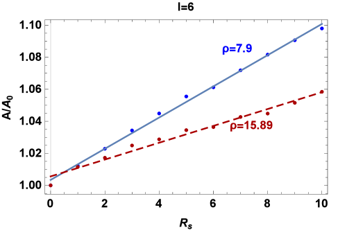
Figure 6: The ratio of the amplitudes of the waves $A/A_{0}$ in the presence of a mass ($A$) and in the absence of the mass ($A_{0}$) as a function of the parameter $R_{s}$, when $\rho=7.9$ and $\rho=15.89$.

The amplitude increases up to $10\%$ when $\rho=7.9$ and $R_{s}=10$, while for $\rho=15.89$ and the same value of $R_{s}$, the increase is about $5\%$. Thus the amplitude increase appears to vary inversely proportional with $\rho$ which is consistent with the fact that the GW gains energy as it enters regions of space with higher curvature.

IV Conclusion

The effects of a point mass on a GW evolving in an expanding universe are determined by the mass $M$ and the physical distance $a\rho$ of the wave from the mass through the expression $\frac{R_{s}}{a\rho}\equiv\frac{2GM}{a\rho}$. In the context of a perturbative weak field analysis we have demonstrated that a point mass tends to increase the amplitude and the period of the GW linearly with respect to $\frac{R_{s}}{a\rho}$. This result is consistent with expectations based on gravitational time delay and energy considerations.

Even though our numerical results were presented for the special case of a radiation dominated cosmological background ($a(\tau)\sim\tau$) and a specific multipole component of the wave ($l=6$) we have checked that their qualitative features persist for all multipole components and cosmological backgrounds provided that the weak field condition (24) is respected. Thus, even though we have considered specific spherical waves in this analysis, we anticipate that our results can also describe a plane wave when expressed as a superposition of spherical waves.

The time slicing we considered corresponds to the coordinate time of the particular metric we used. This coordinate time is particularly interesting and generic as it corresponds to the proper time of a static observer located far away from the point mass or in the absence of the point mass. This is the standard cosmic observer whose observations are consistent with the cosmological principle. Clearly a different choice of time slicing would correspond to a different observer and would lead to a different metric and thus different results.

From the results shown in Fig. 5 and Fig. 6, we conclude that $T=T_{0}(1+\mu R_{s})$ and $A=A_{0}(1+\nu R_{s})$ where $\mu$ and $\nu$ are the slopes of the curves which are approximately equal. Thus we have demonstrated that the energy density of GWs which is proportional to $\omega^{2}A^{2}$ has a weak dependence on $R_{s}$ in the context of our weak field approximation as long as the slopes $\mu$ and $\nu$ are approximately equal.

Our result has interesting implications for the calculation of the RGW spectrum which currently assumes Koh (2010); Corda (2010); Grishchuk (2007); Zhang et al. (2008); Gogoberidze et al. (2007); Buonanno et al. (1997) a smooth homogeneous cosmological background and ignores the presence of mass concentrations which as shown in the present analysis would tend to modify both the magnitude and the shape of this spectrum. A proper stochastic analysis including the effects of mass concentrations on the relic GW spectrum is therefore an interesting extension of the present work.

A distortion of the RGW spectrum is expected due to the presence of point masses on various scales due to the increase of each mode amplitude and decrease of each mode frequency. The effect will be stronger in regions of higher mass concentrations. On scales larger than the galactic scales the role of the point mass could be played by a galaxy while on scales of the solar system the role of the point mass could be played by a planet. In the solar system the effect is expected to be rather weak and beyond the sensitivity of current experiments.

An additional interesting extension could be the drop of the weak field approximation and the use of the full McVittie metric McVittie (1933) for the study of GW evolution in an expanding background and in the vicinity of a black hole allowing for strong gravitational field.

Even though our numerical analysis has been well tested and provides detailed quantitative information on the GW evolution in the presence of expansion and a point mass, an analytical perturbative solution describing this evolution would provide further physical insight and appears to be a tractable useful extension of the present work.

Numerical Analysis Files: The mathematica files used for the production of the figures, as well as the figures may be downloaded from here or upon request from the authors.

References

- Einstein (1916) Albert Einstein, “Approximative Integration of the Field Equations of Gravitation,” Sitzungsber. Preuss. Akad. Wiss. Berlin (Math. Phys.) 1916, 688–696 (1916).
- Einstein (1918) Albert Einstein, “Über Gravitationswellen,” Sitzungsber. Preuss. Akad. Wiss. Berlin (Math. Phys.) 1918, 154–167 (1918).
- Ellis et al. (2016) John Ellis, Nick E. Mavromatos, and Dimitri V. Nanopoulos, “Comments on Graviton Propagation in Light of GW150914,” (2016), arXiv:1602.04764 [gr-qc] .
- Le Tiec and Novak (2016) Alexandre Le Tiec and Jérôme Novak, “Theory of Gravitational Waves,” (2016), arXiv:1607.04202 [gr-qc] .
- Saulson (2011) Peter R. Saulson, “Josh Goldberg and the physical reality of gravitational waves,” Gen. Rel. Grav. 43, 3289–3299 (2011).
- Hulse and Taylor (1975) R. A. Hulse and J. H. Taylor, “Discovery of a pulsar in a binary system,” Astrophys. J. 195, L51–L53 (1975).
- Taylor and Weisberg (1982) J. H. Taylor and J. M. Weisberg, “A new test of general relativity: Gravitational radiation and the binary pulsar PS R 1913+16,” Astrophys. J. 253, 908–920 (1982).
- Press and Thorne (1972) W. H. Press and K. S. Thorne, “Gravitational-wave astronomy,” Ann. Rev. Astron. Astrophys. 10, 335–374 (1972).
- Abbott et al. (2016a) B. P. Abbott et al. (Virgo, LIGO Scientific), “GW150914: The Advanced LIGO Detectors in the Era of First Discoveries,” Phys. Rev. Lett. 116, 131103 (2016a), arXiv:1602.03838 [gr-qc] .
- Abbott et al. (2016b) B. P. Abbott et al. (Virgo, LIGO Scientific), “Observation of Gravitational Waves from a Binary Black Hole Merger,” Phys. Rev. Lett. 116, 061102 (2016b), arXiv:1602.03837 [gr-qc] .
- Kahya and Desai (2016) Emre O. Kahya and Shantanu Desai, “Constraints on frequency-dependent violations of Shapiro delay from GW150914,” Phys. Lett. B756, 265–267 (2016), arXiv:1602.04779 [gr-qc] .
- Wu et al. (2016) Xue-Feng Wu, He Gao, Jun-Jie Wei, Xi-Long Fan, Peter Mészáros, Bing Zhang, Zi-Gao Dai, Shuang-Nan Zhang, and Zong-Hong Zhu, “Testing Einstein’s Equivalence Principle With Gravitational Waves,” (2016), arXiv:1602.01566 [astro-ph.HE] .
- Liu et al. (2016) Molin Liu, Zonghua Zhao, Xiaohe You, Jianbo Lu, and Lixin Xu, “Violation of Einstein’s Equivalence Principle on Gravitational Wave Event GW150914 Associated with GBM Transient GW150914-GBM,” (2016), arXiv:1604.06668 [gr-qc] .
- Yunes et al. (2016) Nicolas Yunes, Kent Yagi, and Frans Pretorius, “Theoretical Physics Implications of the Binary Black-Hole Merger GW150914,” (2016), arXiv:1603.08955 [gr-qc] .
- Branchina and De Domenico (2016) Vincenzo Branchina and Manlio De Domenico, “Simultaneous observation of gravitational and electromagnetic waves,” (2016), arXiv:1604.08530 [gr-qc] .
- Schreck (2016) M. Schreck, “Looking for Lorentz violation with gravitational waves,” (2016), arXiv:1603.07452 [gr-qc] .
- Arzano and Calcagni (2016) Michele Arzano and Gianluca Calcagni, “What gravity waves are telling about quantum spacetime,” Phys. Rev. D93, 124065 (2016), arXiv:1604.00541 [gr-qc] .
- Bicudo (2016) Pedro Bicudo, “Tighter bounds on a hypothetical graviton screening mass from the gravitational wave observation GW150914 at LIGO,” (2016), arXiv:1602.04337 [gr-qc] .
- Collett and Bacon (2016) Thomas E. Collett and David Bacon, “Testing the speed of gravitational waves over cosmological distances with strong gravitational lensing,” (2016), arXiv:1602.05882 [astro-ph.HE] .
- Blas et al. (2016) Diego Blas, Mikhail M. Ivanov, Ignacy Sawicki, and Sergey Sibiryakov, “On constraining the speed of gravitational waves following GW150914,” (2016), arXiv:1602.04188 [gr-qc] .
- García-Bellido et al. (2016) Juan García-Bellido, Savvas Nesseris, and Manuel Trashorras, “Gravitational wave source counts at high redshift and in models with extra dimensions,” (2016), arXiv:1603.05616 [astro-ph.CO] .
- Konoplya and Zhidenko (2016) Roman Konoplya and Alexander Zhidenko, “Detection of gravitational waves from black holes: Is there a window for alternative theories?” Phys. Lett. B756, 350–353 (2016), arXiv:1602.04738 [gr-qc] .
- Moffat (2016) J. W. Moffat, “LIGO GW 150914 Gravitational Wave Detection and Generalized Gravitation Theory (MOG),” (2016), arXiv:1603.05225 [gr-qc] .
- Vainio and Vilja (2016) Jaakko Vainio and Iiro Vilja, “f(R) gravity constraints from gravitational waves,” (2016), arXiv:1603.09551 [astro-ph.CO] .
- Dev and Mazumdar (2016) P. S. Bhupal Dev and A. Mazumdar, “Probing the Scale of New Physics by Advanced LIGO/VIRGO,” Phys. Rev. D93, 104001 (2016), arXiv:1602.04203 [hep-ph] .
- Jaeckel et al. (2016) Joerg Jaeckel, Valentin V. Khoze, and Michael Spannowsky, “Hearing the smoke of dark sectors with gravitational wave detectors,” (2016), arXiv:1602.03901 [hep-ph] .
- Giddings (2016) Steven B. Giddings, “Gravitational wave tests of quantum modifications to black hole structure – with post-GW150914 update,” (2016), arXiv:1602.03622 [gr-qc] .
- Sasaki et al. (2016) Misao Sasaki, Teruaki Suyama, Takahiro Tanaka, and Shuichiro Yokoyama, “Primordial black hole scenario for the gravitational wave event GW150914,” (2016), arXiv:1603.08338 [astro-ph.CO] .
- Bird et al. (2016) Simeon Bird, Ilias Cholis, Julian B. Muñoz, Yacine Ali-Haïmoud, Marc Kamionkowski, Ely D. Kovetz, Alvise Raccanelli, and Adam G. Riess, “Did LIGO detect dark matter?” Phys. Rev. Lett. 116, 201301 (2016), arXiv:1603.00464 [astro-ph.CO] .
- Clesse and García-Bellido (2016) Sebastien Clesse and Juan García-Bellido, “The clustering of massive Primordial Black Holes as Dark Matter: measuring their mass distribution with Advanced LIGO,” (2016), arXiv:1603.05234 [astro-ph.CO] .
- Maselli et al. (2016) Andrea Maselli, Stefania Marassi, Valeria Ferrari, Kostas Kokkotas, and Raffaella Schneider, “Constraining modified theories of gravity with gravitational wave stochastic background,” (2016), arXiv:1606.04996 [gr-qc] .
- Dominik et al. (2012) Michal Dominik, Krzysztof Belczynski, Christopher Fryer, Daniel Holz, Emanuele Berti, Tomasz Bulik, Ilya Mandel, and Richard O’Shaughnessy, “Double Compact Objects I: The Significance of the Common Envelope on Merger Rates,” Astrophys. J. 759, 52 (2012), arXiv:1202.4901 [astro-ph.HE] .
- Dominik et al. (2015) M. Dominik, E. Berti, R. O’Shaughnessy, I. Mandel, K. Belczynski, C. Fryer, D. Holz, T. Bulik, and F. Pannarale, “Double Compact Objects III: Gravitational Wave Detection Rates,” Astrophys. J. 806, 263 (2015), arXiv:1405.7016 [astro-ph.HE] .
- Abbott et al. (2016c) B. P. Abbott et al. (Virgo, LIGO Scientific), “GW150914: Implications for the stochastic gravitational wave background from binary black holes,” Phys. Rev. Lett. 116, 131102 (2016c), arXiv:1602.03847 [gr-qc] .
- Nakama and Suyama (2015) Tomohiro Nakama and Teruaki Suyama, “Primordial black holes as a novel probe of primordial gravitational waves,” Phys. Rev. D92, 121304 (2015), arXiv:1506.05228 [gr-qc] .
- Nakama and Suyama (2016) Tomohiro Nakama and Teruaki Suyama, “Primordial black holes as a novel probe of primordial gravitational waves II: detailed analysis,” (2016), arXiv:1605.04482 [gr-qc] .
- Starobinsky (1979) Alexei A. Starobinsky, “Spectrum of relict gravitational radiation and the early state of the universe,” JETP Lett. 30, 682–685 (1979), [Pisma Zh. Eksp. Teor. Fiz.30,719(1979)].
- Abbott and Harari (1986) L. F. Abbott and D. D. Harari, “Graviton Production in Inflationary Cosmology,” Nucl. Phys. B264, 487–492 (1986).
- Dufaux et al. (2007) Jean Francois Dufaux, Amanda Bergman, Gary N. Felder, Lev Kofman, and Jean-Philippe Uzan, “Theory and Numerics of Gravitational Waves from Preheating after Inflation,” Phys. Rev. D76, 123517 (2007), arXiv:0707.0875 [astro-ph] .
- Allen (1988) Bruce Allen, “The Stochastic Gravity Wave Background in Inflationary Universe Models,” Phys. Rev. D37, 2078 (1988).
- Henriques (2004) Alfredo B. Henriques, “The stochastic gravitational - wave background and the inflation to radiation transition in the early universe,” Class. Quant. Grav. 21, 3057 (2004), [Erratum: Class. Quant. Grav.24,6431(2007)], arXiv:astro-ph/0309508 [astro-ph] .
- Riess et al. (1998) Adam G. Riess et al. (Supernova Search Team), “Observational evidence from supernovae for an accelerating universe and a cosmological constant,” Astron. J. 116, 1009–1038 (1998), arXiv:astro-ph/9805201 [astro-ph] .
- Perlmutter et al. (1999) S. Perlmutter et al. (Supernova Cosmology Project), “Measurements of Omega and Lambda from 42 high redshift supernovae,” Astrophys. J. 517, 565–586 (1999), arXiv:astro-ph/9812133 [astro-ph] .
- Zhang et al. (2005) Yang Zhang, Yefei Yuan, Wen Zhao, and Ying-Tian Chen, “Relic gravitational waves in the accelerating Universe,” Class. Quant. Grav. 22, 1383–1394 (2005), arXiv:astro-ph/0501329 [astro-ph] .
- Izquierdo and Pavon (2004) German Izquierdo and Diego Pavon, “Relic gravitational waves and present accelerated expansion,” Phys. Rev. D70, 084034 (2004), arXiv:astro-ph/0409364 [astro-ph] .
- Grishchuk (1975) L. P. Grishchuk, “Amplification of gravitational waves in an istropic universe,” Sov. Phys. JETP 40, 409–415 (1975), [Zh. Eksp. Teor. Fiz.67,825(1974)].
- Zhao (2007) Wen Zhao, “Improved calculation of relic gravitational waves,” Chin. Phys. 16, 2894–2902 (2007), arXiv:gr-qc/0612041 [gr-qc] .
- Sosa Almazan and Izquierdo (2014) Maria Luisa Sosa Almazan and German Izquierdo, “Late evolution of relic gravitational waves in coupled dark energy models,” Gen. Rel. Grav. 46, 1759 (2014), arXiv:1312.0566 [astro-ph.CO] .
- Balek and Polak (2009) Vladimir Balek and Vratko Polak, “Group velocity of gravitational waves in an expanding universe,” Gen. Rel. Grav. 41, 505–524 (2009), arXiv:0707.1513 [gr-qc] .
- L.Brillouin (1960) L.Brillouin, Wave Propagation Group Velocity (Academic,NY, 1960).
- Fabris and de Borba Goncalves (1998) Julio Cesar Fabris and Sergio Vitorino de Borba Goncalves, “Gravitational waves in an expanding universe,” (1998), arXiv:gr-qc/9808007 [gr-qc] .
- Alekseev and Griffiths (1995) George A. Alekseev and J. B. Griffiths, “Propagation and interaction of gravitational waves in some expanding backgrounds,” Phys. Rev. D52, 4497–4502 (1995).
- Tauber (1984) G. E. Tauber, “GRAVITATIONAL WAVES IN AN EXPANDING UNIVERSE,” Found. Phys. 14, 1169–1183 (1984).
- Waylen (1978) P. C. Waylen, “Gravitational Waves in an Expanding Universe,” Proc. Roy. Soc. Lond. A362, 245–250 (1978).
- Tamayo et al. (2015) David Tamayo, J. A. S. Lima, and D. F. A. Bessada, “Primordial Gravitational Waves Production in Running Vacuum Cosmologies,” (2015), arXiv:1503.06110 [astro-ph.CO] .
- Izquierdo Saez (2005) German Izquierdo Saez, Relic gravitational waves in the expanding Universe, Ph.D. thesis, Barcelona, Autonoma U. (2005), arXiv:gr-qc/0601050 [gr-qc] .
- Hartnett and Tobar (2008) John Hartnett and Michael Tobar, “Properties of gravitational waves in an expanding universe,” in In *Carmeli, M. (ed.): Relativity: Modern large-scale spacetime structure of the cosmos* 283-295 (2008).
- Jackson (1972) J. C. Jackson, “Fingers of God: A critique of Rees’ theory of primoridal gravitational radiation,” Mon. Not. Roy. Astron. Soc. 156, 1P–5P (1972), arXiv:0810.3908 [astro-ph] .
- Ikeda et al. (2015) Taishi Ikeda, Chul-Moon Yoo, and Yasusada Nambu, “Expanding universe with nonlinear gravitational waves,” Phys. Rev. D92, 044041 (2015), arXiv:1505.02959 [gr-qc] .
- Su and Zhang (2012) Daiqin Su and Yang Zhang, “Energy Momentum Pseudo-Tensor of Relic Gravitational Wave in Expanding Universe,” Phys. Rev. D85, 104012 (2012), arXiv:1204.0089 [gr-qc] .
- Alekseev (2016) G. A. Alekseev, “Collision of strong gravitational and electromagnetic waves in the expanding universe,” Phys. Rev. D93, 061501 (2016), arXiv:1511.03335 [gr-qc] .
- Baptista and Gerbal (1982) J. P. Baptista and D. Gerbal, “DISPERSION RELATIONS FOR ZERO HELICITY GRAVITATIONAL WAVES IN A RELATIVISTIC EXPANDING MEDIUM,” J. Phys. A15, 3351–3365 (1982).
- Zeldovich (1992) Ya. B. Zeldovich, My universe: Selected reviews, edited by B. Ya. Zeldovich and M. V. Sazhin (1992).
- McVittie (1933) G. C. McVittie, “The mass-particle in an expanding universe,” Mon. Not. Roy. Astron. Soc. 93, 325–339 (1933).
- Stephani et al. (2003) Hans Stephani, Dietrich Kramer, Malcolm MacCallum, Cornelius Hoenselaers, and Eduard Herlt, Exact Solutions of Einstein’s Field Equations, 2nd ed. (Cambridge University Press, 2003) cambridge Books Online.
- Nesseris and Perivolaropoulos (2004a) S. Nesseris and Leandros Perivolaropoulos, “The Fate of bound systems in phantom and quintessence cosmologies,” Phys. Rev. D70, 123529 (2004a), arXiv:astro-ph/0410309 [astro-ph] .
- Antoniou and Perivolaropoulos (2016) Ioannis Antoniou and Leandros Perivolaropoulos, “Geodesics of McVittie Spacetime with a Phantom Cosmological Background,” Phys. Rev. D93, 123520 (2016), arXiv:1603.02569 [gr-qc] .
- Faraoni and Jacques (2007) Valerio Faraoni and Audrey Jacques, “Cosmological expansion and local physics,” Phys. Rev. D76, 063510 (2007), arXiv:0707.1350 [gr-qc] .
- Nolan (2014) Brien C. Nolan, “Particle and photon orbits in McVittie spacetimes,” Class. Quant. Grav. 31, 235008 (2014), arXiv:1408.0044 [gr-qc] .
- Zhang et al. (2006) Y. Zhang, X. Z. Er, T. Y. Xia, Wen Zhao, and H. X. Miao, “Exact Analytic Spectrum of Relic Gravitational Waves in Accelerating Universe,” Class. Quant. Grav. 23, 3783–3800 (2006), arXiv:astro-ph/0604456 [astro-ph] .
- Nesseris and Perivolaropoulos (2004b) S. Nesseris and Leandros Perivolaropoulos, “A Comparison of cosmological models using recent supernova data,” Phys. Rev. D70, 043531 (2004b), arXiv:astro-ph/0401556 [astro-ph] .
- Koh (2010) Seoktae Koh, “Relic gravitational wave spectrum, the trans-Planckian physics and Horava-Lifshitz gravity,” Class. Quant. Grav. 27, 225015 (2010), arXiv:0907.0850 [hep-th] .
- Corda (2010) Christian Corda, “Information on the inflaton field from the spectrum of relic gravitational waves,” Gen. Rel. Grav. 42, 1323–1333 (2010), [Erratum: Gen. Rel. Grav.42,1335(2010)], arXiv:0909.4133 [gr-qc] .
- Grishchuk (2007) L. P. Grishchuk, “Discovering Relic Gravitational Waves in Cosmic Microwave Background Radiation,” (2007), 10.1007/978-90-481-3735-0-10, arXiv:0707.3319 [gr-qc] .
- Zhang et al. (2008) Y. Zhang, W. Zhao, T. Y. Xia, X. Z. Er, and H. X. Miao, “Relic Gravitational Waves And CMB Polarization In The Accelerating Universe,” Laser astrodynamics, space test of relativity and gravitational-wave astronomy. Proceedings, 3rd International ASTROD Symposium, Beijing, P.R. China, July 13-16, 2006, Int. J. Mod. Phys. D17, 1105–1123 (2008), arXiv:0806.2243 [astro-ph] .
- Gogoberidze et al. (2007) Grigol Gogoberidze, Tina Kahniashvili, and Arthur Kosowsky, “The Spectrum of Gravitational Radiation from Primordial Turbulence,” Phys. Rev. D76, 083002 (2007), arXiv:0705.1733 [astro-ph] .
- Buonanno et al. (1997) Alessandra Buonanno, Michele Maggiore, and Carlo Ungarelli, “Spectrum of relic gravitational waves in string cosmology,” Phys. Rev. D55, 3330–3336 (1997), arXiv:gr-qc/9605072 [gr-qc] .