An Energy Stable Monolithic Eulerian Fluid-Structure Numerical Scheme

Abstract

The conservation laws of continuum mechanics, written in an Eulerian frame, do not distinguish fluids and solids, except in the expression of the stress tensors, usually with Newton’s hypothesis for the fluids and Helmholtz potentials of energy for hyperelastic solids. By taking the velocities as unknown monolithic methods for fluid structure interactions (FSI) are built. In this article such a formulation is analysed when the fluid is compressible and the fluid is incompressible. The idea is not new but the progress of mesh generators and numerical schemes like the Characteristics-Galerkin method render this approach feasible and reasonably robust. In this article the method and its discretisation are presented, stability is discussed through an energy estimate. A numerical section discusses implementation issues and presents a few simple tests.

AMS classification

65M60 (74F10 74S30 76D05 76M25).

Introduction

Currently two methods dominate FSI (Fluid-Structure-Interaction) science: Arbitrary Lagrangian Eulerian (ALE) methods especially for thin structures [30][34] and immersed boundary methods (IBM)[31][12], for which the mathematical analysis is more advanced[6] but the numerical implementations lag behind. ALE for large displacements have meshing difficulties [27] and to a lesser extent with the matching conditions at the fluid-solid interface[25]. Furthermore, iterative solvers for ALE-based FSI methods which rely on alternative solutions of the fluid and the structure parts are subject to the added mass effect and require special solvers[17][8].

Alternatives to ALE and IBM are few. One old method [2][3] has resurfaced recently, the so-called actualized Lagrangian methods for computing structures [24] [28] (see also [11] although different from the present study because it deals mostly with membranes).

Continuum mechanics doesn’t distinguish between solids and fluids till it comes to the constitutive equations. This has been exploited numerically in several studies but most often in the context of ALE[26][22][36].

In the present study, which is a follow-up of [33] and [20], we investigate what Stephan Turek[22] Heil[21] and Wang[38] call a monolithic formulation but here in an Eulerian framework, as in [14][15][35][16], following the displaced geometry of the fluid and the solid. In [14], the authors obtained excellent results with the fully Eulerian formulation adopted here but at the cost of meshing difficulties to handle the Lagrangian derivatives. Here we advocated the Characteristic-Galerkin method and obtain an energy estimate, which is not a proof of stability but a prerequisite for it.

1 Conservation Laws

Let the time dependent computational domain $\Omega_{t}$ be made of a fluid region $\Omega_{t}^{f}$ and a solid region $\Omega_{t}^{s}$ with no overlap: $\overline{\Omega}_{t}=\overline{\Omega}_{t}^{f}\cup\overline{\Omega}_{t}^{s}$, $\Omega_{t}^{f}\cap\Omega_{t}^{s}=\emptyset$ at any times $t\in(0,T)$. At initial time $\Omega_{0}^{f}$ and $\Omega_{0}^{s}$ are prescribed.

Let the fluid-structure interface be $\Sigma_{t}=\overline{\Omega}_{t}^{f}\cap\overline{\Omega}_{t}^{s}$ and the boundary of $\Omega_{t}$ be $\partial\Omega_{t}$. The part of $\partial\Omega_{t}$ on which either the structure is clamped or on which there is a no slip condition on the fluid, that part is denoted by $\Gamma$ and assumed to be independent of time.

The following standard notations are used. For more details see one of a textbook: [10],[29],[2],[1], or the following article: ,[22],[26]. For clarity we use bold characters for vectors and tensors/matrices, with some exceptions, like $x,x^{0}\in{\mathbb{R}}^{d},d=2$ or 3.

• ${\mathbf{X}}:\Omega_{0}\times(0,T)\mapsto\Omega_{t}$: ${\mathbf{X}}(x^{0},t)$, the Lagrangian position at t of $x^{0}$.

• ${\mathbf{u}}=\partial_{t}{\mathbf{X}}$, the velocity of the deformation,

• ${\mathbf{F}}=\nabla^{T}{\mathbf{X}}=((\partial_{x^{0}_{i}}{\mathbf{X}}_{j}))$, the Jacobian of the deformation,

• $J=\hbox{det}_{\mathbf{F}}$.

We denote by $\hbox{tr}_{A}$ and $\hbox{det}_{A}$ the trace and determinant of $A$. To describe the fluid structure system we need the following:

• $\rho={\mathbf{1}}_{\Omega^{f}_{t}}\rho^{f}+{\mathbf{1}}_{\Omega^{s}_{t}}\rho^{s}$, the density,

• $\sigma={\mathbf{1}}_{\Omega^{f}_{t}}\sigma^{f}+{\mathbf{1}}_{\Omega^{s}_{t}}\sigma^{s}$, the stress tensor,

• ${\mathbf{f}}(x,t)$ the density of volumic forces at $x,t$.

• ${\mathbf{d}}={\mathbf{X}}(x^{0},t)-x^{0}$, the displacement.

Finally and unless specified all spatial derivatives are with respect to $x\in\Omega_{t}$ and not with respect to $x^{0}\in\Omega_{0}$. Let $\phi$ a function of $x,t$; as $x={\mathbf{X}}(x^{0},t),~{}x^{0}\in\Omega_{0}$, $\phi$ is also a function of $x^{0}$ and we have:

$$\nabla_{x^{0}}\phi=[\partial_{x^{0}_{i}}\phi]=[\partial_{x^{0}_{i}}{{\mathbf{X}}_{j}}\partial_{x_{j}}\phi]={\mathbf{F}}^{T}\nabla\phi.$$

When ${\mathbf{X}}$ is one-to-one and invertible, ${\mathbf{d}}$ and ${\mathbf{F}}$ can be seen as functions of $(x,t)$ instead of $(x^{0},t)$. They are related by

$${\mathbf{F}}^{T}=\nabla_{x^{0}}{\mathbf{X}}=\nabla_{x^{0}}({\mathbf{d}}+x^{0})=\nabla_{x^{0}}{\mathbf{d}}+{\mathbf{I}}={\mathbf{F}}^{T}\nabla{\mathbf{d}}+{\mathbf{I}},~{}~{}~{}\Rightarrow~{}~{}{\mathbf{F}}=({\mathbf{I}}-\nabla{\mathbf{d}})^{-T}$$

Time derivatives are related by (note the notation ${\mathbb{D}_{t}}$)

$${\mathbb{D}_{t}}\phi:=\frac{d}{dt}\phi({\mathbf{X}}(x_{0},t),t)_{|x={\mathbf{X}}(x_{0},t)}=\partial_{t}\phi(x,t)+{\mathbf{u}}\cdot\nabla\phi(x,t).$$

It is convenient to introduce (note the difference between ${\mathbb{D}_{t}}$ above and ${\mathrm{D}}$ here):

$${\mathrm{D}}{\mathbf{u}}=\nabla{\mathbf{u}}+\nabla^{T}{\mathbf{u}}.$$

Conservation of momentum and conservation of mass take the same form for the fluid and the solid:

$$\rho{\mathbb{D}_{t}}{\mathbf{u}}={\mathbf{f}}+\nabla\cdot\sigma,~{}~{}~{}~{}{\mathbb{D}_{t}}\rho+\rho\nabla\cdot{\mathbf{u}}={\mathbb{D}_{t}}(J\rho)=0,$$

So $J\rho=\rho_{0}$ at all times and

$$J^{-1}\rho_{0}{\mathbb{D}_{t}}{\mathbf{u}}=f+\nabla\cdot\sigma\hbox{ in }\Omega_{t},~{}\forall t\in(0,T),$$ (1.1)

with continuity of ${\mathbf{u}}$ and of $\sigma\cdot{\mathbf{n}}$ at the fluid-structure interface $\Sigma$ in absence of interface constraint like surface tension. There are also unwritten constraints pertaining to the realisability of the map ${\mathbf{X}}$ (see [10],[29]).

Figure 1.1: The geometry of the FLUSTRUK test[16]. The cylinder (in black) is fixed but the flag is a thick compressible Mooney-Rivlin material clamped to the cylinder by its left boundary; the outer rectangle is filled with a fluid which enters from the left $\Gamma_{in}$ and leaves on the right $\Gamma_{out}$; the horizontal boundaries of the outer rectangle are walls, so they form together with the cylinder the boundary $\Gamma_{w}$. The flag is at time zero a rectangle of size $l\times h$. The outer rectangle has size $L\times H$. The center of the circle representing the cylinder is at $(c,c)$ in a frame of reference which has the lower left corner at $(0,0)$; the cylinder has radius $r$ and is fixed.

1.1 Constitutive Equations

We consider a bi-diemsional geometry. For the 3d case, see [9].

• For a Newtonian incompressible fluid : $\sigma^{f}=-p^{f}{\bf I}+\mu^{f}{\mathrm{D}}{\mathbf{u}}$

• For an hyperelastic material : $\sigma^{s}=\rho^{s}\partial_{{\mathbf{F}}}\Psi{\mathbf{F}}^{T}$

where $\Psi$ is the Helmholtz potential which, in the case of a S^t-Venant-Kirchhoff material, is [10]

$$\Psi({\mathbf{F}})=\frac{\lambda^{s}}{2}\hbox{tr}^{2}_{{\mathbf{E}}}+\mu^{s}\hbox{tr}_{{\mathbf{E}}^{2}},~{}~{}{\mathbf{E}}=\frac{1}{2}({\mathbf{F}}^{T}{\mathbf{F}}-{\mathbf{I}})$$ (1.2)

It is easy to see that $\hbox{tr}_{\mathbf{E}}=\frac{1}{2}\hbox{tr}_{{\mathbf{F}}^{T}{\mathbf{F}}}-1$ and

$$\partial_{\mathbf{F}}\hbox{tr}_{{\mathbf{F}}^{T}{\mathbf{F}}} =((\partial_{{\mathbf{F}}_{ij}}\sum_{m,n}F_{m,n}^{2}))=2{\mathbf{F}}~{}~{}\Rightarrow~{}\partial_{\mathbf{F}}\hbox{tr}_{\mathbf{E}}={\mathbf{F}}$$ (1.3)

$$\partial_{\mathbf{F}}\hbox{tr}_{({\mathbf{F}}^{T}{\mathbf{F}})^{2}} =((\partial_{{\mathbf{F}}_{ij}}\sum_{n,m,p,k}F_{n,k}F_{n,m}F_{p,m}F_{p,k}))=4{\mathbf{F}}{\mathbf{F}}^{T}{\mathbf{F}}$$ (1.4)

which implies that $\partial_{\mathbf{F}}\hbox{tr}_{{\mathbf{E}}^{2}}=2{\mathbf{F}}{\mathbf{E}}$. Therefore

$$\partial_{\mathbf{F}}\Psi({\mathbf{F}}){\mathbf{F}}^{T}=(\lambda^{s}\hbox{tr}_{\mathbf{E}}{\mathbf{F}}+2\mu^{s}{\mathbf{F}}{\mathbf{E}}){\mathbf{F}}^{T}$$

which in turn implies that

$$\sigma^{s}=\rho^{s}{\mathbf{F}}(\lambda^{s}\hbox{tr}_{\mathbf{E}}+2\mu^{s}{\mathbf{E}}){\mathbf{F}}^{T}=J^{-1}\rho^{s}_{0}{\mathbf{F}}(\lambda^{s}\hbox{tr}_{\mathbf{E}}+2\mu^{s}{\mathbf{E}}){\mathbf{F}}^{T}$$

For a tensor ${\mathbf{A}}$ define $|{\mathbf{A}}|=\sum_{ij}A^{2}_{ij}$.

Remark 1.

Some authors have a different definition for the Lamé coeficient $\lambda\rho^{s}_{0}\to\lambda$, $\mu\rho^{s}_{0}\to\mu$ which define $\sigma^{s}$.

Proposition 1.

Let $\gamma=\hbox{tr}_{{\mathbf{F}}{\mathbf{F}}^{T}}$; then

$$\gamma=\hbox{tr}_{{\mathbf{F}}{\mathbf{F}}^{T}}=(2-2\nabla\cdot{\mathbf{d}}+|\nabla{\mathbf{d}}|^{2})J^{2},~{}\tilde{\gamma}=\gamma J^{-2}$$

and the following holds

$$\sigma^{s}=\rho^{s}\left(a{\mathbf{I}}+2b({\mathrm{D}}{\mathbf{d}}-\nabla{\mathbf{d}}\nabla^{T}{\mathbf{d}})\right),~{}~{}with$$ (1.5)

$$a=\lambda^{s}(\frac{1}{2}\gamma-1)(\tilde{\gamma}-1)+\mu^{s}(\gamma-J^{2}-1)\tilde{\gamma},$$ (1.6)

$$b=\frac{1}{2}(\frac{\lambda^{s}}{2}+\mu^{s})(\gamma-1)-\frac{\lambda^{s}}{4}$$ (1.7)

Proof

First note that if ${\mathbf{B}}={\mathbf{F}}{\mathbf{F}}^{T}$ then

$$\sigma^{s}=\rho^{s}\Big{[}[\lambda^{s}(\frac{1}{2}\gamma-1)-\mu^{s}]{\mathbf{B}}+\mu^{s}{\mathbf{B}}^{2}\Big{]}$$ (1.8)

Now by the Cayley- Hamilton theorem in 2 dimensions, ${\mathbf{B}}^{2}-\gamma{\mathbf{B}}+J^{2}{\mathbf{I}}=0$. As ${\mathbf{B}}^{-1}=I-{\mathrm{D}}{\mathbf{d}}+\nabla{\mathbf{d}}\nabla^{T}{\mathbf{d}}$ let ${\mathbf{C}}={\mathbf{I}}-{\mathbf{B}}^{-1}={\mathrm{D}}{\mathbf{d}}-\nabla{\mathbf{d}}\nabla^{T}{\mathbf{d}}$. Then

$${\mathbf{B}}=\gamma{\mathbf{I}}-J^{2}{\mathbf{B}}^{-1}=(\gamma-J^{2}){\mathbf{I}}+J^{2}{\mathbf{C}},~{}{\mathbf{B}}^{2}=(\gamma^{2}-(1+\gamma)J^{2}){\mathbf{I}}+\gamma J^{2}{\mathbf{C}}.~{}~{}$$ (1.9)

Therefore

$$\sigma^{s} =\rho^{s}\Big{[}[\lambda^{s}(\frac{1}{2}\gamma-1)-\mu^{s}][(\gamma-J^{2}){\mathbf{I}}+J^{2}{\mathbf{C}}]+\mu^{s}[(\gamma^{2}-(1+\gamma)J^{2}){\mathbf{I}}+\gamma J^{2}{\mathbf{C}}]\Big{]}$$ (1.12)

$$=\rho^{s}\Big{[}[(\lambda^{s}(\frac{1}{2}\gamma-1))(\gamma-J^{2})$$

$$~{}~{}~{}~{}+\mu^{s}\gamma(\gamma-1-J^{2})]{\mathbf{I}}+[\lambda^{s}(\frac{1}{2}\gamma-1)+\mu^{s}(\gamma-1)]J^{2}{\mathbf{C}}\Big{]}$$

$\diamond$

1.2 Variational Monolithic Eulerian Formulation

From now on we limit our analysis to the case $\rho_{0}^{s}$,$\rho_{0}^{f}$ constant.

One must find $({\mathbf{u}},p)$ with ${\mathbf{u}}_{|\Gamma}=0$, ${\mathbf{d}}$ and $\Omega_{t}^{s}$, $\Omega^{f}$, solution for all $(\hat{\mathbf{u}},\hat{p})$ with $\hat{\mathbf{u}}_{|\Gamma}=0$ of

$$\displaystyle\left\{\begin{array}[]{l}\displaystyle\int_{\Omega^{f}_{t}}\Big{[}\rho^{f}{\mathbb{D}_{t}}{\mathbf{u}}\cdot\hat{\mathbf{u}}-p\nabla\cdot\hat{\mathbf{u}}-\hat{p}\nabla\cdot{\mathbf{u}}+\frac{\mu^{f}}{2}{\mathrm{D}}{\mathbf{u}}:{\mathrm{D}}\hat{\mathbf{u}}\Big{]}\cr\displaystyle+\int_{\Omega^{s}_{t}}\rho^{s}\left[{\mathbb{D}_{t}}{\mathbf{u}}\cdot\hat{\mathbf{u}}+b({\mathrm{D}}{\mathbf{d}}-\nabla{\mathbf{d}}\nabla^{T}{\mathbf{d}}):{\mathrm{D}}\hat{\mathbf{u}}+a\nabla\cdot\hat{\mathbf{u}}\right]=\int_{\Omega_{t}}f\cdot\hat{\mathbf{u}}\cr{\mathbb{D}_{t}}{\mathbf{d}}={\mathbf{u}},~{}~{}J^{-1}=\hbox{det}_{{\mathbf{I}}-\nabla{\mathbf{d}}},~{}~{}\rho^{r}=J^{-1}\rho^{r}_{0},\cr\{\dot{x}(t)={\mathbf{u}}(x(t),t),~{}x(0)=x_{0}\in\Omega_{0}^{r}~{}\Rightarrow~{}x(t)\in\Omega_{t}^{r}\},~{}r=s,f.\end{array}\right.$$ (1.17)

For an existence result, up to time $T^{*}$, see [4] [13] (see also [37]), provided a regularization term is added to the formulation to insure that $\partial_{t}{\mathbf{d}}$ has $H^{1}$-regularity; $T^{*}$ is such that the solid does not touch the boundary and $\Sigma_{t}$ does not buckle.

2 Numerical Scheme

For the stability of the numerical scheme, the problem is that even for small displacements the Lamé terms $\mu^{s}\nabla{\mathbf{u}}:\nabla\hat{\mathbf{u}}$+$\lambda^{s}\nabla\cdot{\mathbf{u}}\nabla\cdot\hat{\mathbf{u}}$ are hidden in $b{\mathrm{D}}{\mathbf{d}}:{\mathrm{D}}\hat{\mathbf{u}}$ and $a\nabla\cdot\hat{\mathbf{u}}$ in the above variational formulation (1.17).

But notice that

$$J^{2}=1+2\nabla\cdot{\mathbf{d}}-2\hbox{det}_{\nabla{\mathbf{d}}}+3(\nabla\cdot{\mathbf{d}})^{2}+o(|\nabla{\mathbf{d}}|^{2})$$ (2.18)

$$\gamma=2(1+\nabla\cdot{\mathbf{d}}+(\nabla\cdot{\mathbf{d}})^{2}+\frac{1}{2}|\nabla{\mathbf{d}}|^{2}-2\hbox{det}\nabla{\mathbf{d}})+o(|\nabla{\mathbf{d}}|^{2})$$ (2.19)

$$(\frac{\gamma}{2}-1)(\tilde{\gamma}-1)=\nabla\cdot{\mathbf{d}}-(\nabla\cdot{\mathbf{d}})^{2}-\frac{1}{2}|\nabla{\mathbf{d}}|^{2}-2\hbox{det}\nabla{\mathbf{d}}+o(|\nabla{\mathbf{d}}|^{2})$$ (2.20)

So it makes sense to define

$$c=a-\lambda^{s}\nabla\cdot{\mathbf{d}}$$ (2.21)

To prepare the time discretisation of (1.17) with a given time step $\delta t$, let

$$\bar{\mathbf{d}}={\mathbf{d}}-\delta t{\mathbf{u}}$$ (2.22)

Then (1.17) becomes

$$\left\{\begin{array}[]{l}\displaystyle\int_{\Omega^{f}_{t}}\Big{[}\rho{\mathbb{D}_{t}}{\mathbf{u}}\cdot\hat{\mathbf{u}}-p\nabla\cdot\hat{\mathbf{u}}-\hat{p}\nabla\cdot{\mathbf{u}}+\frac{\mu^{f}}{2}{\mathrm{D}}{\mathbf{u}}:{\mathrm{D}}\hat{\mathbf{u}}\Big{]}\cr\displaystyle+\int_{\Omega^{s}_{t}}\rho\delta t\Big{[}b({\mathrm{D}}{\mathbf{u}}-\nabla\bar{\mathbf{d}}\nabla^{T}{\mathbf{u}}-\nabla{\mathbf{u}}\nabla^{T}\bar{\mathbf{d}}+\delta t\nabla{\mathbf{u}}\nabla^{T}{\mathbf{u}}):{\mathrm{D}}\hat{\mathbf{u}}+\lambda^{s}\nabla\cdot{\mathbf{u}}~{}\nabla\cdot\hat{\mathbf{u}}\Big{]}\cr\displaystyle+\int_{\Omega^{s}_{t}}\rho\Big{[}{\mathbb{D}_{t}}{\mathbf{u}}\cdot\hat{\mathbf{u}}+b({\mathrm{D}}\bar{\mathbf{d}}-\nabla\bar{\mathbf{d}}\nabla^{T}\bar{\mathbf{d}}):{\mathrm{D}}\hat{\mathbf{u}}+(c+\lambda^{s}\nabla\cdot\bar{\mathbf{d}})\nabla\cdot\hat{\mathbf{u}}\Big{]}=\int_{\Omega_{t}}f\cdot\hat{\mathbf{u}}\cr{\mathbb{D}_{t}}{\mathbf{d}}={\mathbf{u}},~{}~{}\rho=\rho_{0}\hbox{det}_{{\mathbf{I}}-\nabla{\mathbf{d}}}.\end{array}\right.$$

Here linear elasticity is visible because the zero order term of $b$ is $\frac{\mu^{f}}{2}$. From now on we do not use $\bar{\mathbf{d}}$ because the Characteristics-Galerkin discretisation of ${\mathbb{D}_{t}}{\mathbf{d}}={\mathbf{u}}$ will give an analogue of (2.22).

2.1 Discretisation of Total Derivatives

Let $\Omega\subset{\mathbb{R}}^{d}$, ${\mathbf{u}}\in{\mathbf{H}}^{1}_{0}(\Omega)=(H^{1}_{0}(\Omega))^{d}$, ($d=2$ here), $t\in(0,T)$ and $x\in\Omega$. Then let $\chi^{t}_{{\mathbf{u}},x}(\tau)$ be the solution at time $\tau$ of

$$\dot{\chi}(\tau)={\mathbf{u}}(\chi(\tau),\tau)\hbox{ with }\chi(t)=x.$$

If ${\mathbf{u}}$ is Lipschitz in space and continuous in time the solution exists. The Characteristics-Galerkin method relies on the concept of total derivative:

$${\mathbb{D}_{t}}{\mathbf{v}}(x,t):=\frac{d}{d\tau}{\mathbf{v}}(\chi(\tau),\tau)|_{\tau=t}=\partial_{t}{\mathbf{v}}+{\mathbf{u}}\cdot\nabla{\mathbf{v}}.$$

Given a time step $\delta t$, let us approximate

$$\chi^{(n+1)\delta t}_{{\mathbf{u}}^{n+1},x}(n\delta t)\approx{\mathbb{Y}}^{n+1}(x):=x-{\mathbf{u}}^{n+1}(x)\delta t$$

Remark 2.

Note also that, as $J\rho$ is convected by ${\mathbf{u}}$, that is $J\rho|_{\chi^{t}_{{\mathbf{u}},x}(\tau),\tau}=J\rho|_{x,t}$, so a consistent approximation is

$$(J^{n}\rho_{n})\circ{\mathbb{Y}}^{n+1}(x)=J^{n+1}(x)\rho_{n+1}(x),~{}x\in\Omega_{n+1}.$$

Thus discretizing the total derivative of ${\mathbf{u}}$ or the one of $\rho_{0}{\mathbf{u}}$ will give the same scheme.

$$\displaystyle\rho_{0}(x)\frac{{\mathbf{u}}^{n+1}(x)-{\mathbf{u}}^{n}({\mathbb{Y}}^{n+1}(x))}{\delta t}=J^{n+1}\rho_{n+1}\frac{{\mathbf{u}}^{n+1}-{\mathbf{u}}^{n}\circ{\mathbb{Y}}^{n+1}}{\delta t}$$ (2.23)

$$\displaystyle=\frac{J^{n+1}\rho_{n+1}{\mathbf{u}}^{n+1}-(J^{n}\rho_{n}{\mathbf{u}}^{n})\circ{\mathbb{Y}}^{n+1}}{\delta t}=\frac{\rho_{0}{\mathbf{u}}^{n+1}-(\rho_{0}{\mathbf{u}}^{n})\circ{\mathbb{Y}}^{n+1}}{\delta t}$$ (2.24)

2.2 Updating the fluid and solid domain

From the definition of ${\mathbb{Y}}$, notice that the only way to be consistent is to define $\Omega_{n+1}$ using ${\mathbf{u}}^{n+1}$, i.e. implicitly, since the later is defined also on $\Omega_{n+1}$:

$$\Omega_{n+1}=({\mathbb{Y}}^{n+1})^{-1}(\Omega_{n})=\{x:~{}{\mathbb{Y}}^{n+1}(x):=x-{\mathbf{u}}^{n+1}(x)\delta t\in\Omega_{n}\}$$

2.3 The Time Discretized Scheme

Let

$$\tilde{\mathbf{d}}^{n}:={\mathbf{d}}^{n}\circ{\mathbb{Y}}^{n+1},~{}{\mathbf{d}}^{n+1}=\tilde{\mathbf{d}}^{n}+\delta t{\mathbf{u}}^{n+1},~{}\rho_{n+1}=\rho_{0}\hbox{det}_{{\mathbf{I}}-\nabla{\mathbf{d}}^{n+1}}.$$ (2.25)

Let $\tilde{b}_{n},\tilde{c}_{n}$ be given by (1.5,2.21) computed with $\tilde{d}^{n}$. The following defines ${\mathbf{u}}^{n+1},p^{n+1}$ with ${\mathbf{u}}^{n+1}|_{\Gamma}=0$: $\forall\hat{\mathbf{u}},\hat{p}$, with $\hat{\mathbf{u}}|_{\Gamma}=0$,

$$\left\{\begin{array}[]{l}\displaystyle\int_{\Omega_{n+1}}\rho_{n+1}\frac{{\mathbf{u}}^{n+1}-{\mathbf{u}}^{n}\circ{\mathbb{Y}}^{n+1}}{\delta t}\cdot\hat{\mathbf{u}}\cr\displaystyle~{}~{}~{}+\int_{\Omega^{f}_{n+1}}\Big{[}-p^{n+1}\nabla\cdot\hat{\mathbf{u}}-\hat{p}\nabla\cdot{\mathbf{u}}^{n+1}+\frac{\mu^{f}}{2}{\mathrm{D}}{\mathbf{u}}^{n+1}:{\mathrm{D}}\hat{\mathbf{u}}\Big{]}\cr\displaystyle+\int_{\Omega^{s}_{n+1}}\rho_{n+1}\delta t\Big{[}\tilde{b}_{n}({\mathrm{D}}{\mathbf{u}}^{n+1}-\nabla\tilde{\mathbf{d}}^{n}\nabla^{T}{\mathbf{u}}^{n+1}-\nabla{\mathbf{u}}^{n+1}\nabla^{T}\tilde{\mathbf{d}}^{n}):{\mathrm{D}}\hat{\mathbf{u}}\cr\displaystyle\hskip 56.9055pt+\lambda^{s}\nabla\cdot{\mathbf{u}}^{n+1}\nabla\cdot\hat{\mathbf{u}}\Big{]}\cr\displaystyle+\int_{\Omega^{s}_{n+1}}\Big{[}\tilde{b}_{n}({\mathrm{D}}\tilde{\mathbf{d}}^{n}-\nabla\tilde{\mathbf{d}}^{n}\nabla^{T}\tilde{\mathbf{d}}^{n}):{\mathrm{D}}\hat{\mathbf{u}}+(\tilde{c}_{n}+\lambda^{s}\nabla\cdot\tilde{\mathbf{d}}^{n})\nabla\cdot\hat{\mathbf{u}}\Big{]}\cr\displaystyle=\int_{\Omega_{n+1}}f\cdot\hat{\mathbf{u}}.\end{array}\right.$$ (2.32)

2.4 Iterative Solution by Fixed Point

The most natural method to solve the above is to freeze some coefficients so as to obtain a well posed linear problem and iterate:

1. Start with ${\mathbf{u}}={\mathbf{u}}^{n}$, ${\mathbb{Y}}(x)=x-{\mathbf{u}}\delta t$, $\Omega^{r}={\mathbb{Y}}^{-1}(\Omega^{r}_{n})$, $r=s,f$.

2. Set $\tilde{\mathbf{d}}^{n}={\mathbf{d}}^{n}\circ{\mathbb{Y}}$, $\tilde{\rho}_{n}=\rho_{0}\hbox{det}_{{\mathbf{I}}-\nabla\tilde{\mathbf{d}}}$; compute $\tilde{b}_{n},\tilde{c}_{n}$.

3. Find ${\mathbf{u}}^{n+1},p^{n+1}$ by solving

   $$\left\{\begin{array}[]{l}\displaystyle\int_{\Omega}\tilde{\rho}_{n}\frac{{\mathbf{u}}^{n+1}-{\mathbf{u}}^{n}\circ{\mathbb{Y}}}{\delta t}\cdot\hat{\mathbf{u}}\cr\displaystyle~{}~{}~{}+\int_{\Omega^{f}}\Big{[}-p^{n+1}\nabla\cdot\hat{\mathbf{u}}-\hat{p}\nabla\cdot{\mathbf{u}}^{n+1}+\frac{\mu^{f}}{2}{\mathrm{D}}{\mathbf{u}}^{n+1}:{\mathrm{D}}\hat{\mathbf{u}}\Big{]}\cr\displaystyle+\int_{\Omega^{s}}\tilde{\rho}_{n}\delta t\Big{[}\tilde{b}_{n}({\mathrm{D}}{\mathbf{u}}^{n+1}-\nabla\tilde{\mathbf{d}}^{n}\nabla^{T}{\mathbf{u}}^{n+1}-\nabla{\mathbf{u}}^{n+1}\nabla^{T}\tilde{\mathbf{d}}^{n}):{\mathrm{D}}\hat{\mathbf{u}}\cr\displaystyle\hskip 56.9055pt+\lambda^{s}\nabla\cdot{\mathbf{u}}^{n+1}\nabla\cdot\hat{\mathbf{u}}\Big{]}\cr\displaystyle+\int_{\Omega^{s}}\Big{[}\tilde{b}_{n}({\mathrm{D}}\tilde{\mathbf{d}}^{n}-\nabla\tilde{\mathbf{d}}^{n}\nabla^{T}\tilde{\mathbf{d}}^{n}):{\mathrm{D}}\hat{\mathbf{u}}+(\tilde{c}_{n}+\lambda^{s}\nabla\cdot\tilde{\mathbf{d}}^{n})\nabla\cdot\hat{\mathbf{u}}\Big{]}\cr\displaystyle=\int_{\Omega}f\cdot\hat{\mathbf{u}}\end{array}\right.$$ (2.39)

4. Set ${\mathbf{u}}={\mathbf{u}}^{n+1},{\mathbb{Y}}(x)=x-{\mathbf{u}}\delta t,\Omega^{r}={\mathbb{Y}}^{-1}(\Omega^{r}_{n}),~{}r=s,f$.

5. If not converged return to Step 2 else set ${\mathbf{d}}^{n+1}={\mathbf{d}}^{n}\circ{\mathbb{Y}}+\delta t{\mathbf{u}}^{n+1}$.

Notice that (2.39) is a well posed linear problem whenever

$$A({\mathbf{u}},\hat{\mathbf{u}})=\int_{\Omega^{s}}\left[\frac{\rho}{\delta t}{\mathbf{u}}\cdot\hat{\mathbf{u}}+\tilde{b}({\mathrm{D}}{\mathbf{u}}-\nabla\tilde{\mathbf{d}}^{n}\nabla^{T}{\mathbf{u}}-\nabla{\mathbf{u}}\nabla^{T}\tilde{\mathbf{d}}^{n}):{\mathrm{D}}\hat{\mathbf{u}}+\lambda^{s}\nabla\cdot{\mathbf{u}}\nabla\cdot\hat{\mathbf{u}}\right]$$

is coercive. Then (2.39) gives a solution bounded in ${\mathbf{H}}^{1}(\Omega)$ and converging subsequences can be extracted from $\rho_{n+1},{\mathbf{u}}^{n+1},\Omega^{r}_{n+1}$ when $\bar{\Omega}=\overline{\Omega^{f}_{n}\cup\Omega^{s}_{n}}$ is fixed. Then convergence would occur if we could prove that $\Omega^{r}_{n+1}$ converges.

2.5 Spatial Discretisation with Finite Elements

Let ${\mathcal{T}}_{h}^{0}$ be a triangulation of the initial domain. Spatial discretisation can be done with the most popular finite element for fluids: the Lagrangian triangular elements of degree 2 for the space $V_{h}$ of velocities and displacements and Lagrangian triangular elements of degree 1 for the pressure space $Q_{h}$; later we will also discuss the stabilised $P^{1}-P^{1}$ element; provision must be made for two pressure variables, one in the structure and one in the fluid because the pressure is discontinuous at the interface $\Sigma$; therefore $Q_{h}$ is the space of piecewise linear functions on the triangulation continuous in $\Omega^{r}_{n+1},~{}r=s,f$. A small penalization with parameter $\epsilon$ must be added to impose uniqueness of the pressure.

This leads us to find ${\mathbf{u}}^{n+1}_{h}\in V_{h0_{\Gamma}}$, $p^{n+1}_{h}\in Q_{h}$, $\Omega_{n+1}$ such that for all $\hat{\mathbf{u}}_{h},\hat{p}_{h}\in V_{h0_{\Gamma}}\times Q_{h}$ with

$$\tilde{\mathbf{d}}_{h}^{n}:={\mathbf{d}}_{h}^{n}\circ{\mathbb{Y}}^{n+1},~{}\hbox{ where }{\mathbb{Y}}^{n+1}(x)=x-{\mathbf{u}}^{n+1}_{h}(x)\delta t,$$

the following holds:

$$\left\{\begin{array}[]{l}\displaystyle{\bf a}(\tilde{\rho}_{n},\tilde{b}_{n},\tilde{c}_{n};{\mathbf{u}}^{n+1},\hat{\mathbf{u}}):=\int_{\Omega_{n+1}}\tilde{\rho}_{n}\frac{{\mathbf{u}}_{h}^{n+1}-{\mathbf{u}}_{h}^{n}\circ{\mathbb{Y}}^{n+1}}{\delta t}\cdot\hat{\mathbf{u}}_{h}\cr\displaystyle~{}~{}~{}+\int_{\Omega^{f}_{n+1}}\Big{[}-p^{n+1}\nabla\cdot\hat{\mathbf{u}}_{h}-\hat{p}\nabla\cdot{\mathbf{u}}_{h}^{n+1}+\frac{\mu^{f}}{2}{\mathrm{D}}{\mathbf{u}}_{h}^{n+1}:{\mathrm{D}}\hat{\mathbf{u}}_{h}\Big{]}\cr\displaystyle+\int_{\Omega^{s}_{n+1}}\tilde{\rho}^{s}_{n}\delta t\Big{[}\tilde{b}_{n}({\mathrm{D}}{\mathbf{u}}_{h}^{n+1}-\nabla\tilde{\mathbf{d}}_{h}^{n}\nabla^{T}{\mathbf{u}}_{h}^{n+1}-\nabla{\mathbf{u}}_{h}^{n+1}\nabla^{T}\tilde{\mathbf{d}}_{h}^{n}):{\mathrm{D}}\hat{\mathbf{u}}_{h}\cr\displaystyle\hskip 56.9055pt+\lambda^{s}\nabla\cdot{\mathbf{u}}_{h}^{n+1}\nabla\cdot\hat{\mathbf{u}}_{h}\Big{]}\cr\displaystyle+\int_{\Omega^{s}_{n+1}}\Big{[}\tilde{b}_{n}({\mathrm{D}}\tilde{\mathbf{d}}_{h}^{n}-\nabla\tilde{\mathbf{d}}_{h}^{n}\nabla^{T}\tilde{\mathbf{d}}_{h}^{n}):{\mathrm{D}}\hat{\mathbf{u}}_{h}+(\tilde{c}_{n}+\lambda^{s}\nabla\cdot\tilde{\mathbf{d}}_{h}^{n})\nabla\cdot\hat{\mathbf{u}}_{h}\Big{]}\cr\displaystyle=\int_{\Omega_{n+1}}{\mathbf{f}}\cdot\hat{\mathbf{u}}_{h},~{}~{}~{}~{}~{}~{}\Omega_{n+1}=({\mathbb{Y}}^{n+1})^{-1}(\Omega_{n})=\{x:~{}{\mathbb{Y}}^{n+1}(x)\in\Omega_{n}\}.\end{array}\right.$$ (2.46)

Then ${\mathbf{d}}$

$${\mathbf{d}}_{h}^{n+1}=\tilde{\mathbf{d}}_{h}^{n}+\delta t{\mathbf{u}}_{h}^{n+1},$$

2.6 Implementation

The various tests we made lead us to recommend the following:

• Move the vertices of the mesh in the structure with its own velocity:

  $$q^{n+1}_{i}=q^{n}_{i}+{\mathbf{u}}_{h}^{n+1}(q^{n+1}_{i})\delta t$$ (2.47)

  which, as explained above has to be implemented through an iterative process.

• Remesh the fluid part at each iteration with a Delaunay-Voronoi mesh generator from the boundary vertices ($\Sigma_{n+1}$ included).

  This required the development of a specific module to identify computationally the vertices of the fluid-structure interface $\Sigma$, which are then input to the fluid mesh generator.

• In doing so, the discrete topological properties of the structural part are preserved and we have the important property that the value ${\mathbf{d}}[i]$ of ${\mathbf{d}}$ at vertex $q_{i}$ in the computer implementation of ${\mathbf{d}}$ by an array of values at the nodes, satisfies

  $${\mathbf{d}}^{n+1}[i]={\mathbf{d}}^{n}[i]+\delta t{\mathbf{u}}^{n+1}[i],~{}~{}\forall i.$$

  In other words ${\mathbf{d}}^{n}\circ{\mathbb{Y}}^{n+1}$ is ${\mathbf{d}}^{n}[i]$ after moving the vertices by (2.47).

3 Energy Estimate

3.1 Stability of the Scheme Discretized in Time

To conserve energy we need to change the scheme (2.46) slightly, from

$${\bf a}(\tilde{\rho}_{n},\tilde{b}_{n},\tilde{c}_{n};{\mathbf{u}}^{n+1},\hat{\mathbf{u}})=\int_{\Omega_{n+1}}{\mathbf{f}}\cdot\hat{\mathbf{u}}_{h}~{}\hbox{ to }$$ (3.48)

$${\bf a}(\rho_{n+1},b_{n+1},c_{n+1};{\mathbf{u}}^{n+1},\hat{\mathbf{u}})+\delta t^{2}\int_{\Omega^{s}_{n+1}}\rho^{s}_{n+1}b_{n+1}\nabla{\mathbf{u}}_{h}^{n+1}\nabla^{T}{\mathbf{u}}_{h}^{n+1}:{\mathrm{D}}\hat{\mathbf{u}}_{h}~{}~{}$$ (3.49)

$$=\int_{\Omega_{n+1}}{\mathbf{f}}\cdot\hat{\mathbf{u}}_{h}$$ (3.50)

Lemma 3.1.

The mapping ${\mathbf{X}}^{n}:\Omega_{0}\mapsto\Omega_{n}$ is also ${\mathbf{X}}^{n+1}=({\mathbb{Y}}^{n+1})^{-1}\circ{\mathbf{X}}^{n}$, $n\geq 1$ and the jacobian of the transformation is ${\mathbf{F}}^{n}:=\nabla^{T}_{x_{0}}{\mathbf{X}}^{n}=({\mathbf{I}}-\nabla{\mathbf{d}}^{n})^{-T}$.

Proof

Notice that ${\mathbb{Y}}^{1}({\mathbb{Y}}^{2}(..{\mathbb{Y}}^{n-1}({\mathbb{Y}}^{n}(\Omega_{n}))..))=\Omega_{0}$ Hence

$${\mathbf{X}}^{n+1}=[{\mathbb{Y}}^{1}({\mathbb{Y}}^{2}(..{\mathbb{Y}}^{n}({\mathbb{Y}}^{n+1})))]^{-1}=({\mathbb{Y}}^{n+1})^{-1}\circ{\mathbf{X}}^{n}.$$

By definition of ${\mathbf{d}}^{n+1}$ in (2.25)

$${\mathbf{d}}^{n+1}({\mathbf{X}}^{n+1}(x_{0})) ={\mathbf{d}}^{n}({\mathbb{Y}}^{n+1}({\mathbf{X}}^{n+1}(x_{0})))+{\mathbf{u}}^{n+1}({\mathbf{X}}^{n+1}(x_{0}))\delta t$$ (3.52)

$$={\mathbf{d}}^{n}({\mathbf{X}}^{n}(x_{0}))+{\mathbf{u}}^{n+1}({\mathbf{X}}^{n+1}(x_{0}))\delta t,$$

and since ${\mathbf{X}}^{n+1}(x_{0})={\mathbf{d}}^{n+1}({\mathbf{X}}^{n+1}(x_{0}))+x_{0}$ we have that

$${{\mathbf{F}}^{n+1}} ={\nabla^{t}_{x_{0}}}({\mathbf{d}}^{n+1}(({\mathbf{X}}^{n+1}(x_{0})))+x_{0}),$$ (3.54)

$$={\nabla{\mathbf{d}}^{n+1}}^{T}{\mathbf{F}}^{n+1}+{\mathbf{I}}~{}\Rightarrow~{}{\mathbf{F}}^{n+1}=({\mathbf{I}}-\nabla{\mathbf{d}}^{n+1})^{-T}$$

$\diamond$

Note that (3.52) shows also that

$${\mathbf{F}}^{n+1}={\mathbf{F}}^{n}+\delta t\nabla_{x_{0}}^{T}{\mathbf{u}}^{n+1}$$ (3.55)

Lemma 3.2.

With $\Psi$ defined by (1.2),

$$\displaystyle\int_{\Omega^{s}_{n+1}}\rho^{s}_{n+1} \left[b^{n+1}({\mathrm{D}}{\mathbf{d}}^{n+1}-\nabla{\mathbf{d}}^{n+1}\nabla^{T}{\mathbf{d}}^{n+1}):{\mathrm{D}}\hat{\mathbf{u}}+a^{n+1}\nabla\cdot\hat{\mathbf{u}}\right]$$ (3.57)

$$=\int_{\Omega^{s}_{0}}\partial_{{\mathbf{F}}}\Psi^{n+1}:\nabla_{x_{0}}\hat{\mathbf{u}}$$

Proof By Proposition 1 and Lemma 3.1:

$$\displaystyle\int_{\Omega^{s}_{n+1}}\rho^{s}_{n+1}\left(a^{n+1}{\mathbf{I}}+2b^{n+1}({\mathrm{D}}{\mathbf{d}}^{n+1}-\nabla{\mathbf{d}}^{n+1}\nabla^{T}{\mathbf{d}}^{n+1})\right):\nabla\hat{\mathbf{u}}$$ (3.58)

$$=\int_{\Omega^{s}_{n+1}}\sigma^{s}_{n+1}:\nabla\hat{\mathbf{u}}=\int_{\Omega^{s}_{n+1}}\left[\rho^{s}_{n+1}\partial_{{\mathbf{F}}}\Psi{\mathbf{F}}^{T}\right]|_{n+1}:\nabla\hat{\mathbf{u}}$$ (3.59)

$$=\int_{\Omega^{s}_{n+1}}\left[J_{n+1}^{-1}\rho^{s}_{0}\partial_{{\mathbf{F}}}\Psi{\mathbf{F}}^{T}\right]|_{n+1}:\nabla\hat{\mathbf{u}}=\int_{\Omega^{s}_{0}}\rho^{s}_{0}\partial_{{\mathbf{F}}}\Psi^{n+1}:\nabla\hat{\mathbf{u}}$$ (3.60)

$\diamond$

Theorem 3.3.

When $f=0$ and $\rho_{0}$ is constant in each domain $\Omega^{r}_{0},~{}r=s,f$, the numerical scheme (3.48) has the following property:

$$\int_{\Omega_{n}}\frac{\rho_{n}}{2}|{\mathbf{u}}^{n}|^{2}+\delta t\sum_{k=1}^{n}\int_{\Omega_{k}^{f}}\frac{\mu^{f}}{2}|{\mathrm{D}}{\mathbf{u}}^{k}|^{2}+\int_{\Omega^{s}_{0}}\Psi^{n}\leq\int_{\Omega_{0}}\frac{\rho_{0}}{2}|{\mathbf{u}}^{0}|^{2}+\int_{\Omega^{s}_{0}}\Psi^{0}$$ (3.61)

Proof Let $r=s$ or $f$. Let us choose $\hat{\mathbf{u}}={\mathbf{u}}^{n+1}$ in (3.48). By Schwartz inequality

$$\int_{\Omega^{r}_{n+1}}\rho_{n+1}({\mathbf{u}}^{n}\circ{\mathbb{Y}}^{n+1})\cdot{\mathbf{u}}^{n+1}=\rho_{0}\int_{\Omega^{r}_{n+1}}(J^{n+1})^{-1}({\mathbf{u}}^{n})\circ{\mathbb{Y}}^{n+1})\cdot{\mathbf{u}}^{n+1}$$

$$\leq\rho_{0}\left(\int_{\Omega^{r}_{n+1}}(J^{n+1})^{-1}({\mathbf{u}}^{n}\circ{\mathbb{Y}}^{n+1})^{2}\right)^{\frac{1}{2}}\left(\int_{\Omega^{r}_{n+1}}(J^{n+1})^{-1}({\mathbf{u}}^{n+1})^{2}\right)^{\frac{1}{2}}$$

$$=\left[\int_{\Omega^{r}_{n}}\rho_{n}({\mathbf{u}}^{n})^{2}\int_{\Omega^{r}_{n+1}}\rho_{n+1}({\mathbf{u}}^{n+1})^{2}\right]^{\frac{1}{2}}\leq\frac{1}{2}\int_{\Omega^{r}_{n}}\rho^{r}_{n}{{\mathbf{u}}^{n}}^{2}+\frac{1}{2}\int_{\Omega^{r}_{n+1}}\rho^{r}_{n+1}{{\mathbf{u}}^{n+1}}^{2},$$

Plugging this estimate in (3.48) with $\hat{\mathbf{u}}={\mathbf{u}}^{n+1}$ leads to

$$\int_{\Omega_{n+1}}\frac{\rho_{n+1}}{2}|{\mathbf{u}}^{n+1}|^{2}+\delta t\int_{\Omega^{f}_{n+1}}\frac{\mu^{f}}{2}|{\mathrm{D}}{\mathbf{u}}^{n+1}|^{2}+\int_{\Omega_{0}}\Psi^{n+1}\leq\int_{\Omega_{n}}\frac{\rho_{n}}{2}|{\mathbf{u}}^{n}|^{2}+\int_{\Omega_{0}}\Psi^{n}$$

$\diamond$

3.2 Energy Estimate for the Fully Discrete Scheme

The proof for the spatially continuous case will work for the discrete case if

$${\mathbf{X}}^{n}={\mathbf{X}}^{n+1}\circ{\mathbb{Y}}^{n+1}.$$ (3.62)

As discussed in [20] it may be possible to program an isoparametric $P^{2}-P^{1}$ element for which (3.62) but it is certainly far from easy. On the other hand, consider the stabilised $P^{1}-P^{1}$ element: the fluid pressure and the solid pressure are continuous and piecewise linear on the triangulation. The inf-sup condition for stability does not hold unless the incompressibility condition in the fluid, $\nabla\cdot{\mathbf{u}}=0$, is changed to $-\epsilon\Delta p+\nabla\cdot{\mathbf{u}}=0$, (see [5] for details). It amounts to adding $\epsilon\nabla p^{n+1}\nabla\hat{p}$ next to the term with $\mu^{f}$ in the variational formulations.

Figure 3.2: Sketch to understand if ${\mathbf{X}}^{n}={\mathbb{Y}}^{n+1}\circ{\mathbf{X}}^{n+1}$ holds with the $P^{1}-P1$ stabilised element. A triangle $T^{k}_{0}$ in the reference domain (chosen here to be its initial position at time zero) becomes triangle $T^{k}_{n}$ at $t_{n}$ and $T^{k}_{n+1}$ at time $t_{n+1}$: $T^{k}_{n}={\mathbf{X}}^{n}(T^{k}_{0})$ and $T^{k}_{n+1}={\mathbf{X}}^{n+1}(T^{k}_{0})$ Vertices are preserved by these transformations.

Then (3.62) holds (see Figue 3.2) and the proof of the spatially continuous case can be adapted leading to (3.61) with an additional viscous term $\epsilon|\nabla p^{n+1}|^{2}$ next to the term with $\mu^{f}$.

Remark 3.

Because of energy preservation scheme (3.48), implemented via a fixed point algorithm as in (2.39), generates bounded sequences $\rho,{\mathbf{u}},q^{i}$; it seems safe to assess that out of these bounded subsequences will converge to a solution of the problem discretized in space but continuous in time when $\delta t\to 0$.

4 Numerical Tests

In our tests we have used the $P^{2}-P^{1}$ element, confident that it will behave as well as the stabilised $P^{1}-P1$ element as indicated in [20].

4.1 The Cylinder-Flag Test

A compressible hyperelastic Mooney-Rivlin material, shaped as a rectangle of size $[0,l]\times[0,h]$, is attached behind a cylinder of radius $r$ and beats in tune with the Karman vortices of the wake behind the cylinder; the fluid in the computational rectangular domain $[0,L]\times[0,H]$ enters from the left and is free to leave on the right. The center of the cylinder is at $(c,c)$ (see figure 1.1). In [14] the following numerical values are suggested:

Geometry

$l=0.35$, $h=0.02$, $L=2.5$, $H=0.41$, $c=0.2$ which puts the cylinder slightly below the symmetry line.

Fluid

density $\rho^{f}=10^{3}kg/m^{3}$ and a reduced viscosity $\displaystyle\nu^{f}=\frac{\mu^{f}}{\rho^{f}}=10^{-3}m^{2}/s$; inflow horizontal velocity $\displaystyle{\mathbf{u}}(0,y)=\bar{U}\left(\frac{6}{H^{2}}y(H-y),0\right)^{T}$ is a parabolic profile with flux $\bar{U}H$. Top and bottom boundaries are walls with no-slip conditions.

Solid

$\displaystyle E=2\mu(1+\sigma)/\rho^{s}$, $\sigma=0.4$, $\displaystyle\lambda=\frac{E\sigma}{(1+\sigma)(1-2\sigma)}$.

Initial velocities and displacements are zero. In all cases the same mesh is used initially with 2500 vertices. The time step is 0.005.

4.1.1 Free Fall of a Thick Flag

The gravity is $g=9.81$ in $\Omega_{t}$. When $\bar{U}=0$, $\mu=0.13510^{6}$ and $\rho^{s}=20\rho^{f}$, the flag falls under its own weight; it comes to touch the lower boundary with zero velocity at time 0.49 and then moves up under its spring effect. This test is named FLUSTRUK-FSI-2^∗ in [14] but we have used a different value for $\mu$ because the one reported in [14] seems unlikely.

Figure 4.4 shows a zoom around the flag at the time when it has stopped to descend and started to move upward. Pressure lines are drawn in the flow region together with the mesh and the velocity vectors in the flag and drawn at each vertex. Figure 4.4 shows the coordinates of the upper right tip of the flag versus time.

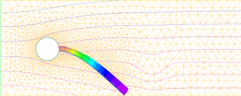
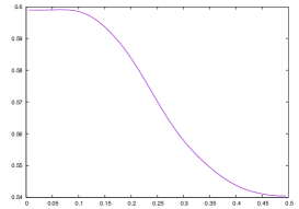
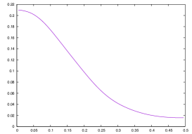
Figure 4.3: FLUSTRUK-FSI-2^∗[14]. Zoom near the flag at t=0.495 just as it begins to move up after the fall under its own weight in a flow initially at rest.Mesh and Pressure lines are shown in the fluid and velocity vectors in the solid.

Figure 4.4: FLUSTRUK-FSI-2^∗ test of [14]. Position of the upper right corner of the flag versus time: x vs t on the left and y vs t on the right.

4.1.2 Flow past a Cylinder with a Thick Flag Attached

This test is known as FLUSTRUK-FSI-3 in [14]. The geometry is the same as above but now $\bar{U}=2$, $\mu=210^{6}$ and $\rho^{s}=\rho^{f}$. After some time a Karman-Vortex alley develops and the flag beats accordingly. Results are shown on Figures 4.5 and 4.6; the first one displays a snapshot of the velocity vector norms and the second the y-coordinate versus time of the top right corner of the flag.

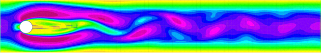
Figure 4.5: FLUSTRUK-FSI-3 Test. Color map based on the norm of the fluid and solid velocity vectors

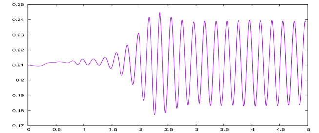
Figure 4.6: FLUSTRUK-FSI-3 Test. Vertical position of the upper right tip of the flag versus time shown up to t=5

These numerical results compare reasonably well with those of [14]. The frequency is $5s^{-1}$ compared to $5.04$ and the maximum amplitude 0.031 compared to 0.032. However the results are sensitive to the time step.

Conclusion

A fully Eulerian fluid-structure formulation has been presented for compressible materials with large displacements, discretized by an implicit first order Euler Scheme and the $P^{2}-P^{1}$ or stabilised $P^{1}-P^{1}$ elements. An energy estimate has been obtained which guarantees the stability of the scheme so long as the motion of the vertices does not flip-over a triangle. The method has been implemented with FreeFem++[19]. It is reasonably robust when the vertices in the structure are moved by their velocities and the fluid is remeshed with an automatic Delaunay mesh generator. The method is first order in time and therefore somewhat too diffusive for delicate tests. It is being extended to 3D and to second order in time discretisation.

Acknowledgement

The author thanks Frédéric Hecht for very valuable discussions and comments.

References

• [1] S.S. Antman. Nonlinear Problems of Elasticity ($2^{nd}$ ed.). Springer series in Applied Mathematical Sciences, Vol. 107, 2005.
• [2] K.J. Bathe. Finite element procedures, Prentice-Hall, Englewood Cliffs, New-Jersey. 1996.
• [3] K.J. Bathe, E. Ramm and E. L. Wilson. Finite Element Formulations for Large Deformation Dynamic Analysis. Int. J. Numer. Methods Eng., 9(2) :353-386, 1975.
• [4] M. Boulakia, Existence of weak solutions for the motion of an elastic structure in an incompressible viscous fluid, C. R. Math. Acad. Sci. Paris 336 No 12 (2003), 985-990.
• [5] D. Boffi, F. Brezzi, M. Fortin. Mixed Finite Element Methods and Applications. Springer Series in Computational Mathematics 44, Berlin 2013.
• [6]  D. Boffi, N. Cavallini, L. Gastaldi, The finite element immersed boundary method with distributed lagrange multiplier, arXiv:1407.5184v2, 2015 (to appear)
• [7] K. Boukir, Y. Maday, B. Metivet. A high order characteristics method for the incompressible Navier-Stokesequations. Comp. Methods in Applied Mathematics and Engineering 116 (1994), 211-218.
• [8] M. Bukaca, S. Canic, R. Glowinski, J. Tambacac, A. Quainia. Fluid-structure interaction in blood flow capturing non-zero longitudinal structure displacement. Journal of Computational Physics 235 (2013) 515-541.
• [9] Chiang Chen-Yu, Olivier Pironneau, Tony Sheu, Marc Thiriet. Numerical Study of a 3D Eulerian Monolithic Formulation for Fluid-Structure-Interaction. Submitted to Fluids an MDPI publication (2017).
• [10] P.G. Ciarlet. Mathematical Elasticity. North Holland, 1988.
• [11] G.H. Cottet, E. Maitre, T. Milcent. Eulerian formulation and level set models for incompressible fluid-structure interaction. M2AN Math. Model. Numer. Anal. 42 (2008), no. 3, 471-492.
• [12] Th. Coupez, L. Silva, E. Hachem, Implicit Boundary and Adaptive Anisotropic Meshes, S. Peretto, L. Formaggia eds. New challenges in Grid Generation and Adaptivity for Scientific Computing. SEMA-SIMAI Springer series, vol 5, 2015.
• [13] D. Coutand and S. Shkoller, Motion of an elastic solid inside an incompressible viscous fluid, Arch. Ration. Mech. Anal. 176 No 1 (2005), 25-102.
• [14] Th. Dunne, Adaptive Finite Element Approximation Of Fluid-Structure Interaction Based On An Eulerian Variational Formulation, ECCOMAS CFD 2006 P. Wesseling, E. Oñate and J. Périaux (Eds) Elsevier, TU Delft, The Netherlands, 2006.
• [15] Th. Dunne. An Eulerian approach to fluid-structure interaction and goal-oriented mesh adaptation. Int. J. Numer. Meth. Fluids 2006; 51:1017-1039.
• [16] Th. Dunne and R. Rannacher Adaptive Finite Element Approximation of Fluid-Structure Interaction Based on an Eulerian Variational Formulation. In Fluid-Structure Interaction: Modelling, Simulation,Optimization. Lecture Notes in Computational Science and Engineering, vol 53. p110-146, H-J. Bungartz, M. Schaefer eds. Springer 2006.
• [17] M. A. Fernandez, J. Mullaert, M. Vidrascu. Explicit Robin-Neumann schemes for the coupling of incompressible fluids with thin-walled structures, Comp. Methods in Applied Mech. and Engg. 267, 566-593, 2013.
• [18] P. Hauret. Méthodes numériques pour la dynamique des structures non-linéaires incompressibles à deux échelles. Doctoral thesis, Ecole Polytechnique, 2004.
• [19] F. Hecht New development in FreeFem++, J. Numer. Math., 20 (2012), pp. 251-265. www.FreeFem.org.
• [20] F. Hecht and O. Pironneau. An Energy Preserving Monolithic Eulerian Fluid-Structure Finite Element Method: the incompressible case. (submitted to IJNMF (2016)).
• [21] Matthias Heil, Andrew L. Hazel, Jonathan Boyle Solvers for large-displacement fluid structure interaction problems: segregated versus monolithic approaches. Comput Mech (2008) 43:91-101
• [22] J. Hron and S. Turek. A monolithic fem solver for an ALE formulation of fluid-structure interaction with configuration for numerical benchmarking. European Conference on Computational Fluid Dynamics ECCOMAS CFD 2006 P. Wesseling, E. Onate and J. Periaux (Eds). TU Delft, The Netherlands (2006)
• [23] C. Kane, J.E. Marsden, M. Ortiz, and M. West. Variational integrators and the Newmark algorithm for conservative and dissipative mechanical systems. International Journal for Numerical Methods in Engineering, 49 :1295-1325, 2000.
• [24] S. Léger. Méthode lagrangienne actualisée pour des problèmes hyperélastiques en très grandes déformations. Thèse de doctorat, Université Laval, 2014.
• [25] P. Le Tallec and P. Hauret. Energy conservation in fluid-structure interactions. In P. Neittanmaki Y. Kuznetsov and O. Pironneau, editors, Numerical methods for scientific computing, variational problems and applications, CIMNE, Barcelona, 2003.
• [26] P. Le Tallec and J. Mouro. Fluid structure interaction with large structural displacements. Comp. Meth. Appl. Mech. Eng., 190(24-25) :3039-3068, 2001.
• [27] J. Liu. A second-order changing-connectivity ALE scheme and its application to FSI with large convection of fluids and near-contact of structures. Submitted to Journal of Computational Physics, (2015).
• [28] I-Shih Liu, R. Cipolatti and M. A. Rincon. Incremental linear approximation for finite elasticity. Proc ICNAAM 2006, WIley.
• [29] J. Marsden and T.J.R. Hughes Mathematical Foundations of Elasticity. Dover publications 1993.
• [30] F. Nobile, C. Vergara. An effective fluid-structure interaction formulation for vascular dynamics by generalized robin conditions. SIAM J. Sci. Comp., 30(2):731–763, 2008.
• [31] C.S. Peskin. The immersed boundary method. Acta Numerica, 11:479-517, 2002.
• [32] O. Pironneau. Finite Element Methods for Fluids. Wiley, 1989.
• [33] O. Pironneau. Numerical Study of a Monolithic Fluid-Structure Formulation. i Variational Analysis and Aerospace Engineering: Mathematical Challenges for the Aerospace of the Future Aldo Frediani, Bijan Mohammadi, Olivier Pironneau (eds). Springer 2016.
• [34] L. Formaggia, A. Quarteroni, A. Veneziani. Cardiovasuclar Mathematics. Springer MS&A Series. Springer-Verlag, 2009.
• [35] R. Rannacher and T. Richter, An Adaptive Finite Element Method for Fluid-Structure Interaction Problems Based on a Fully Eulerian Formulation. Springer Lecture Notes in Computational Science and Engineering, Vol 73, 2010.
• [36] Th. Richter and Th. Wick. Finite elements for fluid-structure interaction in ALE and fully Eulerian coordinates. Comput. Methods Appl. Mech. Engrg. 199 (2010) 2633-2642.
• [37] Jean-Pierre Raymond, Muthusamy Vanninathan A fluid-structure model coupling the Navier-Stokes equations and the Lamé system. J. Math. Pures Appl. 102 (2014) 546-596
• [38] Yongxing Wang The Accurate and Efficient Numerical Simulation of General Fluid Structure Interaction: A Unified Finite Element Method. Proc. Conf. on FSI problems, IMS-NUS, Singapore, June 2016, Jie Liu ed.