Glimpses of stellar surfaces. II. Origins of the photometric modulations and timing variations of KOI-1452

The deviations of the mid-transit times of an exoplanet from a linear ephemeris are usually the result of gravitational interactions with other bodies in the system. However, these types of transit timing variations (TTV) can also be introduced by the influences of star spots on the shape of the transit profile.
Here we use the method of unsharp masking to investigate the photometric light curves of planets with ambiguous TTV to compare the features in their $O-C$ diagram with the occurrence and in-transit positions of spot-crossing events. This method seems to be particularly useful for the examination of transit light curves with only small numbers of in-transit data points, i.e., the long cadence light curves from Kepler satellite.
As a proof of concept we apply this method to the light curve and the estimated eclipse timing variations of the eclipsing binary KOI-1452, for which we prove their non-gravitational nature. Furthermore, we use the method to study the rotation properties of the primary star of the system KOI-1452 and show that the spots responsible for the timing variations rotate with different periods than the most prominent periods of the system’s light curve. We argue that the main contribution in the measured photometric variability of KOI-1452 originates in g-mode oscillations, which makes the primary star of the system a $\gamma$-Dor type variable candidate.

1 Introduction

One of the most efficient ways to study the physical parameters of an exoplanet is by studying their transits in front of their parent star. As shown by Agol et al. (2005), it is even possible to infer the existence of additional low-mass and otherwise unobservable companions with the measurement of the mid-transit times and their deviations from linear period ephemeris. Depending on the actual planetary configuration, these transit timing variations (TTV) can reach differences up to a few hours with respect to the linear period ephemeris of the planet, especially for systems close to low order mean motion resonances. Although additional system components can also be inferred from precise radial velocity (RV) measurements, the importance of the TTV method increases with the number of planets around fainter stars, where the quality of RV measurements is decreasing. While the measurements of TTV are possible with ground-based observations, the high accuracy, continuous light curves from the CoRoT (Baglin et al. 2006) and Kepler (Koch et al. 2010) space missions provide evidence for statistically significant TTV in more than 60 cases.

Despite its success, the study of exoplanets with the method of transits using high precision photometry can be somewhat problematic in the case of active host stars. The transit profile of planets orbiting around spotted stars become distorted when the planet is passing over dark star spots during its transit (e.g., Rabus et al. (2009), Wolter et al. (2009)). The severity of this effect can be such that quite large systematic errors are introduced in the calculation of the physical parameters of the planets (see Czesla et al. (2009) and Oshagh et al. (2013)). Furthermore, Ioannidis et al. (2016) show that the influence of these spot-crossing events on the estimates of the mid-transit times of a planet can lead to statistically significant false positive TTV detections under certain conditions, and there are several cases where the detected low-amplitude TTV are actually believed to be caused by spot-crossing events (e.g., Sanchis-Ojeda et al. (2011), Fabrycky et al. (2012), Szabó et al. (2013), Mazeh et al. (2013)). Likewise, Kalimeris et al. (2002) predict that eclipse timing variations (ETV) may be caused by spot-crossing events in the eclipses of close binaries with at least one photospherically active component (e.g., Tran et al. 2013)

The identification of the spot-crossing events and their correlation with the TTV of a planet can be cumbersome, especially for planets with small periods and thus a large number of transits. Here we show that the method of unsharp masking, i.e., examining the transit light curve produced by subtracting out the mean transit model (see Sect. 2) is a suitable tool to compare the measured $O-C$ mid-transit time variations with the transit light curves and to identify correlations between the occurrence of spot-crossing events and the measured TTV. To demonstrate the power of this method, we present a case study of the TTV of KOI-1452 in Sect. 3, and finally we discuss our results in Sect. 4, and summarize with our conclusions in sect. 5.

Figure 1: Top: Consecutive simulated transits of a planet with an orbital period $P_{\mathrm{orb}}$ = 1.0132 $P_{\star}$. Each light curve is affected by spot-crossing events; see text for details.
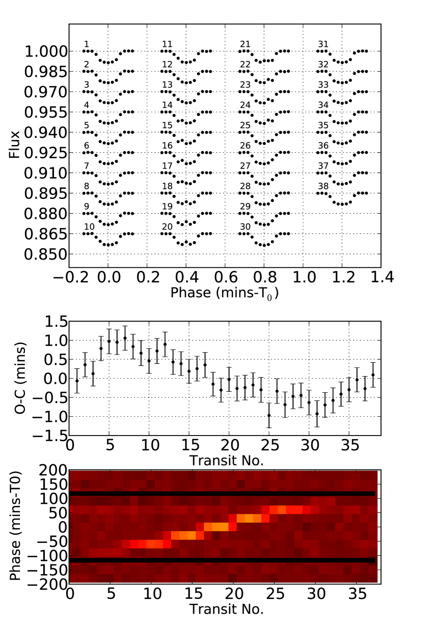
Middle: Estimated mid-transit times of the transits in the top panel. The sinusoidal shape of the $O-C$ diagram is the result of spot-crossing anomalies in the transits Ioannidis et al. (2016).
Bottom: Unsharp masking transit residuals of the planet; note the correlation with the sinusoidal O-C diagram in the middle panel.

2 Unsharp masking of transit light curves

As discussed by Ioannidis et al. (2016), when planets cross over cool star spots during the transit, the resulting transit profiles show an increment of stellar flux compared to a pristine un-spotted transit. Owing to the continuous evolution of starspots, these spot-induced in-transit anomalies are usually not included in the model fit of the transit light curve. As a result, the spot-crossing events can potentially alter the mid-transit time estimate, which is derived using a spot-free transit light curve. The position of the spot-crossing event in the transit profile influences the amplitude and the sign of the spot-induced variation. The resulting maximal amplitude of this fake TTV depends on the physical properties of the star, the planet, and the spot.

In consecutive transits of the same planet, the position of the spot-crossing event can change from one transit to the next, depending on the period ratio between the orbital period $P_{\mathrm{orb}}$ and rotational period $P_{\mathrm{rot}}$ of the star. Fake TTV may result if $P_{\mathrm{orb}}$ and $P_{\mathrm{rot}}$ are not identical. In particular, the time needed for a spot to cross the total transit profile is equal to half of the beating period and it is given by the expression

$$D_{\mathrm{sp}}={P_{\mathrm{orb}}\over{2}}\cdot\left({P_{\mathrm{orb}}\over P_{\mathrm{rot}}}-1\right)^{-1},$$ (1)

assuming parallel orbital and rotational axes. Sometimes it is useful to express the value of D_sp from Eq. 1 in terms of the number of transits needed for a spot crossing, which is given by

$$D_{\mathrm{sp\_tr}}={{D_{\mathrm{sp}}}\over{P_{\mathrm{orb}}}}.$$ (2)

The sign of D_sp value is related the direction of the spot motion: If D_sp¿0, the spot crossing events occur in the direction from transit ingress towards egress ($P_{\mathrm{orb}}>P_{\mathrm{rot}}$) and vice versa. We note that this relation between the sign of D_sp and the spot motion in consecutive transits is valid for a prograde planetary orbit; in the case of a retrograde orbit, the above correlation is reversed.

To demonstrate the effects of spot-crossing events we carry out a simulation of a sequence of transits with a spot-crossing event. The simulation is geared towards a typical transit signal-to-noise ratio (TSNR) and integration times of a long cadence Kepler light curve of a star with magnitude $K_{p}=13$ mag (Jenkins et al. 2010). We specifically assume a ratio between the orbital period of the planet $P_{\mathrm{orb}}$ and the rotational period of the star $P_{\mathrm{rot}}$ of $P_{\mathrm{orb}}/P_{\mathrm{rot}}$ = 1.0132. We further assume a dark star spot ($R_{\mathrm{sp}}=0.06\,R_{\mathrm{\star}}$) on the visible hemisphere and that is kept fixed on the stellar surface, which is occulted by the planet ($R_{\mathrm{pl}}=0.08\,R_{\mathrm{\star}}$) during every consecutive transit. The resulting transit light curves are shown in the top panel of Figure 1. Since orbital and rotational periods differ slightly, the position of the spot-crossing event slowly changes from one transit to the next, which leads to changes in the derived mid-transit times shown in the middle panel of Fig. 1.

The identification of the spot-crossing events and the correlation of their occurrence and in-transit position to the $O-C$ diagram is one of the most efficient ways to distinguish between real and spot-induced TTV. Although we know that the $O-C$ variations in Fig. 1 are produced by spot crossing events, it is not trivial to locate the in-transit anomalies that are responsible for each one of the TTV. Given the correct global parameters for the transit model, the light curve residuals, calculated by subtracting the model from the data, should appear featureless and just show un-correlated noise. Yet, when spot-crossing events occur, clearly visible features appear (see Fig. 1, bottom panel), which are straightforward to identify, and using the unsharp masking method provides an easy juxtaposition of the in-transit anomalies with the $O-C$ diagram; furthermore it can reveal important information regarding photospheric structures (e.g., cold spots) in the band of the star that is occulted by the planet.

Figure 2: Top: Part of KOI-1452 light curve. There are clear periodic variations, suggesting the appearance of spots in the visible stellar hemispheres (see text for details). The primary eclipses are indicated with green markers.
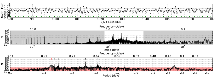
Middle: The L-S periodogram of the total Kepler light curve. The unshaded part around the area with the most significant periodicities is shown enlarged in the lower panel.
Bottom: The red shaded area shows the values of the periodogram with false alarm probability higher than 10^-3. The four most prominent periods of the L-S periodogram with periods of $P_{1}$ = 1.516 days, $P_{2}$ = 1.4097 days, $P_{3}$ = 1.1978 days and $P_{4}$ = 1.1702 days are indicated by black arrows, while the red arrow indicates the orbital period of the system ($P_{\mathrm{orb}}$ = 1.1522 days).

3 Application: KOI-1452

Table 1: System parameters for KOI-1452.

KIC	7449844
Kepler (mag)	13.630
J (mag)	12.727
Period (days)	1.152 $\pm$ 7$\cdot 10^{-6}$∗
RB/RA	0.122 $\pm$ 0.002 ∗
a/RA	2.858 $\pm$ 0.012 ∗
i	73.189$\degree$ $\pm$ 0.085$\degree$∗
LB/LA	$7.14\times 10^{-4}\pm 3.53\times 10^{-4}$∗
MA ($M_{\mathrm{\odot}}$)	1.6 $\pm$ 0.3∗
MB ($M_{\mathrm{\odot}}$)	0.2 $\pm$ 0.1∗
RA ($R_{\mathrm{\odot}}$)	2.0 $\pm$ 0.1 ∗
RB ($R_{\mathrm{\odot}}$)	0.3 $\pm$ 0.1∗
a ($\mathrm{au}$)	0.0265 $\pm$ 0.0015 ∗
T${}_{\mathrm{eff_{A}}}$	7 268 $\pm$ 487 †
T${}_{\mathrm{eff_{B}}}$	3 582 $\pm$ 546 †
Age (Myr)	10 - 20 ∗

^∗ calculated in this work
^† calculated by Armstrong et al. (2014)

3.1 Light curve analysis

In the following, we apply the unsharp masking technique to the Kepler data of KOI-1452. KOI-1452 was first listed as planet host candidate by the Kepler satellite survey after the identification of a transit-like signal with a period of $P_{\mathrm{orb}}$ = 1.1522 days. We show the Kepler light curve of KOI-1452 in the upper panel of Fig. 2, which demonstrates that, in addition to the transit-like signals (shown with ticks) the light curve of KOI-1452 shows significant modulations of the order of $\sim$2%, suggesting an active star, like CoRoT-2 (see Alonso et al. 2008 and Huber et al. 2009). Analyzing these modulations with a Lomb-Scargle (L-S) periodogram (Zechmeister & Kürster 2009), shown in the middle panel of Fig. 2, we find a plethora of significant periodicities with the most prominent peak at $P_{\mathrm{rot}}\simeq$ 1.516 days, and the equally separated peaks in the frequency domain with periods smaller than one day that can be identified as harmonics of the orbital period $P_{orb}$.

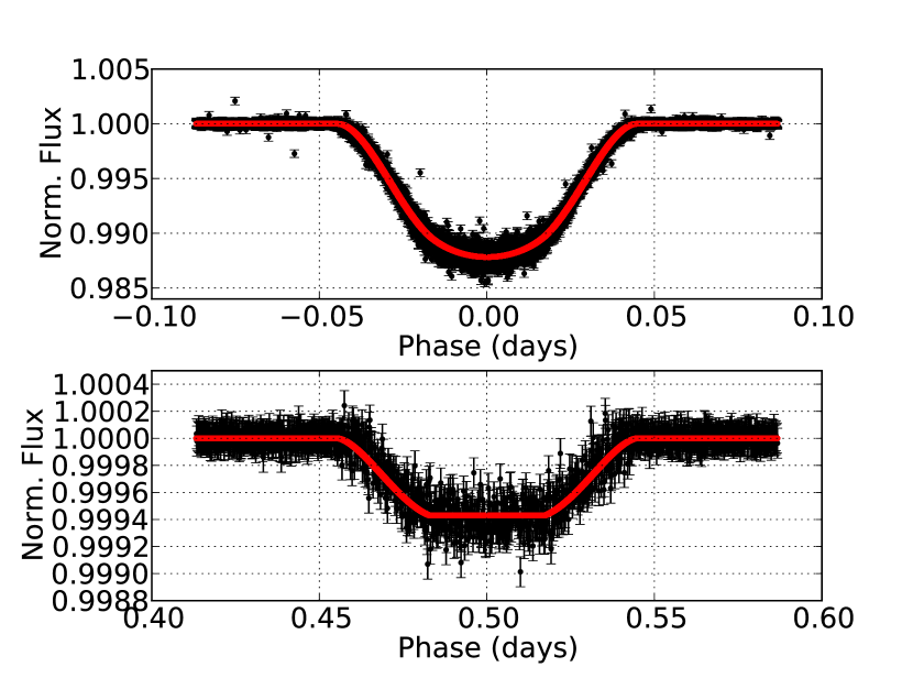
Soon after its detection with the Kepler satellite, the KOI-1452 system was, however, categorized as a stellar binary system owing to the presence of visible secondary eclipses in its light curve (Slawson et al. 2011). In Fig. 3, we show the primary (upper panel) and secondary (lower panel) eclipses of KOI-1452, phase folded using the calculated period $P_{\mathrm{orb}}=$1.152 days; the model shown as a red curve in Fig. 3 is constructed using the analytical eclipse light curve model by Mandel & Agol (2002) and a summary of our model-fit results is given in Table 1. Clearly, the shape of the primary eclipse looks very similar to that of a planetary transit. The model of the secondary eclipse (red curve in the lower panel of Fig. 3) requires identical parameters as the model calculated from the primary eclipse, assuming an inverted flux ratio and mid-transit times. The increased dispersion of the in-transit data points is an indication of spot-crossing events in the light curves (see, Czesla et al. (2009)). We finally note that, according to the studies of Lillo-Box et al. (2014), Teske et al. (2015) and Kolbl et al. (2015), there is no evidence of companions in angular distances smaller than 2”, therefore we do not consider third light contamination.

Figure 3: Phase folded primary (top) and secondary (bottom) eclipses of KOI-1452 (black dots) and the global eclipse model (red line); see text for details.

Figure 4: Top: Radial velocity measurements of KOI-1452 phased with the orbital period $P_{\mathrm{orb}}$ = 1.1522 days. The red line shows the expected RV curve for a system of an F-type and an early M-type star, primary eclipses occur in phase zero. The expected RV amplitude of K$\sim 75\,km\,s^{-1}$ agrees well with the data, excluding the possibility for the companion to be a planet.
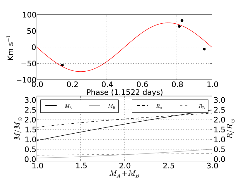
Bottom: Estimated masses (solid lines) and radii (dashed lines) for the components of the system as a function of the total mass $\mathrm{M_{A}+M_{B}}$; see text for details.

3.2 Stellar characteristics

The flat-bottom shape of the secondary eclipse (see Fig. 3) shows that the fainter companion is totally eclipsed by the primary star. Retrieving radial velocity (RV) data for the KOI-1452 system from the public archive CFOP (https://cfop.ipac.caltech.edu) and folding the data with the orbital period $P_{\mathrm{orb}}$ = 1.1522 days, we can construct an (admittedly sparse) RV curve for KOI-1452, shown in the top panel of Fig. 4, which suggests an RV semi-amplitude of K$\simeq 75\,km\,s^{-1}$. With this value of K we use the mass function and Kepler’s third law in combination with the measured values for the orbital inclination $i$ and radius ratio $R_{\mathrm{B}}/R_{\mathrm{A}}$ (see Table 1) to calculate an estimate for the components’ masses and radii of the system components as a function of the assumed total system mass. The resulting curves are shown in the lower panel of Fig. 4. Using the observed color index ($B-V\simeq 0.4$), we can set a constraint for the total system mass in the range ${1.6\,M_{\odot}\lesssim\,\mathrm{M}_{\mathrm{A}}+\mathrm{M}_{\mathrm{B}}\,\lesssim 2.2\,M_{\odot}}$. For values of total mass outside this range, the expected mass-radius combinations appear to be unusual. Using our estimates for the mass, the radius, and the temperature of the system components, we are able to set constraints regarding the age of the system between $\sim$10 Myr and $\sim$20 Myr, using the isochrones derived by Siess et al. (2000) and Bressan et al. (2012).

Comparing the flux reductions observed during the primary and secondary eclipse, we calculate the ratio of the effective temperatures of the two components as T${}_{\mathrm{eff_{A}}}=2.11$ T${}_{\mathrm{eff_{B}}}$. This estimate is in good agreement with the T_eff values calculated by Armstrong et al. (2014).

Taking into account the masses and radii estimates (see, Fig. 4) in combination with the ratio of the effective temperatures, we argue that the system consists of a slightly inflated F-type star and an M-dwarf star.

3.3 False positive timing variations

The preparation of the Kepler light curves and the ETV analysis follow the same principles described by Ioannidis et al. (2016). In the top panel of Fig. 5, we plot the $O-C$ diagram of KOI-1452, which shows clear variations with an amplitude of $\sim$2-3 mins (Mazeh et al. (2013) and Szabó et al. (2013)). In addition, the LS-periodogram (Zechmeister & Kürster 2009) of the derived $O-C$ values, shown in the bottom panel of Fig. 5, reveals a variety of high power periodicities, with the most prominent peak at a period $P_{O-C}\approx$71 days. The coordination of the rotation period of the system, in combination with the small number of in-transit points, periodically affect the mid-transit timing measurements; this effect is visible as the high peak close to $\sim$3 days in the L-S periodogram.

Figure 5: $O-C$ diagram of KOI-1452 (top) and its L-S periodogram (bottom). Many significant signal periods between 60 and 100 days appear, the peak close to 3 days is caused by the data sampling.

Figure 6: Top: Part of $O-C$ diagram of KOI-1452 between 1000 days $\leq$ BJD (+2454833) $\leq$ 1070 days.
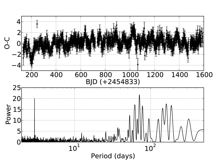
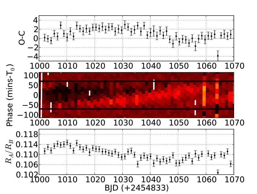
Middle: Concurrent unsharp masking transit light curve residuals. The bright stripe is due to spot-crossing anomalies, which change their position from one transit to the next due to the small period difference (cf., Fig. 1). The white areas indicate no data. The black lines indicate the first and fourth contact of the eclipse.
Bottom: Variation of the measured radii $R_{\mathrm{B}}/R_{\mathrm{A}}$ for each eclipse. During the strongest observed TTV the star appears to be larger because of spot coverage during the transit (Czesla et al. 2009).

In Fig. 6 we zoom in on a small portion of the $O-C$ diagram of KOI-1452 in that part of the light curve between 1 000 days $\leq$ BJD (+2454833) $\leq$ 1 070 days to juxtapose the phased light curve residuals with the the $O-C$ diagram and the derived stellar parameters. We choose this particular part of the light curve since, in that time period, the clearest features in the $O-C$ diagram are found. The bright, stripe-shaped feature is the result of many spot-crossing events, which appear in different, in-transit positions owing to the small difference between the orbital and rotational periods. A comparison between the $O-C$ diagram and the phased unsharp masked light curve shows that the ETV occur at the same time as those features, in good agreement with our simulations (see Fig. 1). The discrepancies of the $O-C$ diagram and our simulation are introduced by other spots, in different positions in the transit profile (e.g., a new feature appears in the phased color plot after BJD (+2454833) $\simeq$ 1 040 days).

As a second step, we calculate the depth for each observed eclipse; the relative measurements for KOI-1452 are presented in the bottom panel of Fig. 6. According to Czesla et al. (2009), the presence of cold spots during the transit of a planet, or in this case the eclipse of an other so-called cold star, can cause an overestimate of its radius. As a result, when the occulting body appears to be larger than average (increased transit/eclipse depth), the possibility of a spot-crossing event occurrence also increases. The comparison of the bottom panel of Fig. 6 with the top and middle panels shows the correlation of the individual occultation depths with the measured ETVs of the system and the existence of spot-crossing events, respectively.

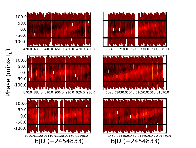
Spot-crossing events are visible during the total Kepler light curve of KOI-1452, with similar characteristics and correlation to the measured ETV and eclipse depth. Additional examples of these types of spot-crossing events in the eclipses of KOI-1452 are shown in Fig. 7.

4 Discussion

4.1 The different periods of KOI-1452

As far as the observed light curve modulations of KOI-1452 are concerned, the most straightforward interpretation would be to attribute them to starspots and one would interpret the different peaks in the L-S diagram as indicators of differential rotation (e.g., Reinhold et al. 2013). While F-type stars do not usually show high levels of photospheric activity, the inflated state of the KOI-1452 main component - because of its youth - allows us to consider such a possibility. Also, if KOI-1452 is a very active star, as suggested by its Kepler light curve (see Fig. 3), one would also expect spot-crossing events as observed, for example, for CoRoT-2 (e.g., Wolter et al. 2009, Czesla et al. 2009 and Huber et al. 2010) and, indeed, our unsharp masking analysis (see Figs. 6 and 7) does suggest spot-crossing events. Considering the spots that are involved in spot-crossing events and using the average of the $D_{\mathrm{sp}}$ values of the spot crossing features shown in Fig. 7, we estimate $D_{\mathrm{sp}}\simeq 35\pm 5$ days; we note that the sign of $D_{\mathrm{sp}}$ is positive since we observe the spots drifting with a direction from ingress to egress (see Sect. 2). Using Eq. 1, we then compute the period of the spots responsible for the spot-crossing features in the eclipses of KOI-1452 as $P_{\mathrm{rot}}=\,1.1357\pm 0.003$ days, assuming a prograde orbit, or $P_{\mathrm{rot}}=\,1.1687\pm 0.003$ days, assuming a retrograde orbit.

Despite the relatively young age of the system (see Table 1) we estimate - using the formulation derived by Zahn (1977) - that the synchronization and circularization processes should occur much earlier in the lifetime of the system (i.e., $\tau_{\mathrm{circ}}\lesssim$1 Myr). In combination with the light curve modeling results (i.e., the eclipses have equal durations and they are separated by half orbital period $P_{\mathrm{orb}}$ as shown in Fig. 3), it is reasonable to assume that the two stars are tidally locked, i.e., the rotational periods of (actually both) stars coincide with the orbital period of the system, and thus the rotational periods ought to be close to 1.15 days. However, the highest peak in the LS periodogram is found at $P_{\mathrm{rot}}\simeq$ 1.512 days (cf., Fig 2). If this peak was produced by star spots rotating with this period, these spots cannot be responsible for the spot-crossing events observed in the transits of KOI-1452, since for this period ratio the difference between the transit positions of the spots in consecutive transits would be much greater. Using Eq. 2, we calculate that a spot with a period of $P_{\mathrm{rot}}\simeq$ 1.512 days requires $D_{\mathrm{sp\_tr}}=-1.6$ rotations to cover the total transit profile, which would lead to two problems: first, these spots would not be visible continuously from one rotation to the next, resulting in completely different ETV patterns and spot-crossing features, and second, the spots should occur with a direction from egress to ingress, opposite to the direction in which they appear to drift (see Fig. 7).

Figure 7: Collection with the clearest spot-crossing features from the light curve of KOI-1452; white regions are due to data absence. The black lines indicate the first and fourth contact of the eclipse.

4.2 Differential rotation ?

In Fig. 8, we show an artist’s impression of the KOI-1452 system during a primary eclipse, using the estimated orbital characteristics shown in Table 1 and assuming that rotational and orbital angular momenta are aligned. The semi-transparent black band represents the eclipsed part of the primary in the stellar latitude range between $25\degree\lesssim\phi_{\star}\lesssim 50\degree$. The equatorial regions at $0\degree$ are assumed to rotate with a period of 1.15 days.

Figure 8: An impression of the KOI-1452 system during a primary eclipse. The horizontal lines indicate the latitudes of the system’s primary, which appears tilted according to our hypothesis of zero system obliquity. The semi-transparent band represents the latitudes occulted during an eclipse.

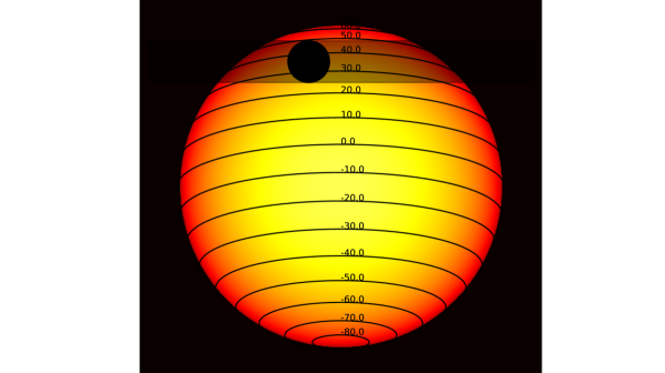
It is hard to see where regions rotating with 1.51 days should be located on the star, and also the level of differential rotation required (period difference of $\sim$30% between neighboring latitudes) is very large. Balbus & Weiss (2010) discuss the possibility of zonal stellar surface flows, i.e., flows similar to those observed on the surfaces of the giant planets in our solar system. Following this hypothesis would lead to accounting for the non-linear evolution of the differential rotation along the stellar latitude. As a result, this might explain the required rapid alternations in the rotation period. Also, in the case of the giant planets in the solar system, the velocity differences observed in the zonal bands are in the percent range, but not 30%.

An even more exotic hypothesis would be that the differential rotation of the star is opposite to that of the Sun, i.e., the star rotates more slowly in the equator. Anti-solar differential rotation would explain the fact that the spots occulted by the companion spots, which are slower, appear in high latitudes. In addition, it would explain the dominance of the slow spots in the modulations of the light curve, as they would appear closer to the equator and thus larger (as a result of the projection effect). Although this is a plausible explanation, anti-solar differential rotation is proposed for evolved stars (Brun & Palacios 2009).

4.3 Gravity-mode pulsations ?

Both the area of the Hertzsprung-Russell diagram, where the main component of the KOI-1452 system is located, and the nature of the periodicities found in the Kepler light curve, make it a candidate for a $\gamma$-Dor type variable star. These stars are F-type stars with effective temperatures of between $\sim$6 900 K and $\sim$7 500 K, which lie on or just above the main sequence. They are slightly more massive than the Sun (1.4-2.5$M_{\odot}$) and show multi-periodic oscillations with periods between 0.3 and 3 days, which are the result of gravity-mode (g-mode) pulsations (e.g., Kaye et al. 1999). The mechanism responsible for the g-mode pulsations is related to the fluctuations of the radiative flux at the base of the convective envelope of the stars (Guzik et al. 2000). Assuming a non-rotating star with a chemically homogeneous radiative envelope, one should expect pulsations with identical spherical degree $l$ and a variety of radial orders $n$ with equidistantly spaced periods (Tassoul 1980). Furthermore, stellar rotation introduces frequency splitting, which results in separated period spacing patterns, relative to the azimuthal order $m$. Van Reeth et al. (2015) present a survey of several dozens of $\gamma$-Dor variable stars. While the majority of these stars have slightly shorter pulsation periods and have period spacings again somewhat shorter than the period spacing of P$\leavevmode\nobreak\ =\leavevmode\nobreak\$0.1063 days observed for KOI-1452 (see bottom panel of Fig. 2), the observed parameters for KOI-1452 do not fall completely outside the range observed for $\gamma$ Dor variable stars. While an in-depth asteroseismic analysis of KOI-1452 is beyond the scope of this paper, the hypothesis that stellar pulsations and not stellar activity is responsible for the observed light curve modulations of KOI-1452, appears to be the simplest hypothesis and would not require the introduction of somewhat exotic differential rotation scenarios. Yet, the spot-crossing events visible in the primary eclipses of the binary suggest that, in addition, activity modulations must exist which are probably described by the part of the L-S periodogram in the period range between 1.13 days and 1.17 days.

4.4 Retrograde orbit ?

The assumption that the most dominant features in the L-S periodogram of the KOI-1452 system are the result of g-mode pulsations could explain the large discrepancy between the measured periodicities, i.e., the difference between $P_{\mathrm{orb}}$ and $P_{1}$ in Fig. 2. However, the fact that the spot-crossing features in the eclipses of KOI-1452 rotate with $P_{\mathrm{rot}}=\,1.1357\pm 0.003$ days or $P_{\mathrm{rot}}=\,1.1687\pm 0.003$ days, assuming a prograde or retrograde orbit respectively, requires some additional discussion.

There is no feature in the L-S periodogram close to period with value $P_{\mathrm{rot}}=\,1.1357\pm 0.003$ days. Yet there is a peak in the L-S periodogram at a period $P_{\mathrm{rot}}=\,1.1687\pm 0.003$ days. Since the value of this peak is very close to the suggested rotational period of the occulted spots $P_{\mathrm{rot}}=\,1.1687\pm 0.003$ days, it is tempting to identify the two. However, this requires us to assume that the primary star rotates in the opposite direction of the orbital motion of its companion, which is in contradiction to the hypothesis of tidal locking.

5 Summary

In this paper, we discuss the technique of unsharp masking as a tool for transit light curve analysis to locate spot-crossing anomalies and compare their occurrence with the estimated $O-C$ diagram of the mid-transit times. We apply the method to the Kepler light curve of KOI-1452, where we show the correlation between the timing variations and spot-crossing events in the primary eclipses of the system.

Furthermore, we use the same method to show that it is possible to extract information about the properties of the spots, which are occulted during a transit/eclipse. As a result, we argue that the spots occulted by the faint companion in the KOI-1452 system are very likely not responsible for the modulations in the Kepler light curve of the system. We argue, furthermore, that the hypothesis that KOI-1452 is a $\gamma$-Dor variable can naturally explain the light curve variability for periods of 1.19 days and longer, while star spots are responsible for the spot-crossing events in the primary eclipses of the system and might explain the 1.17 days feature in the periodogram. Clearly, ground-based observations are called for to better determine the physical parameters of the KOI-1452 system. A more densely sampled RV curve would yield more precise estimates of the component masses, a high-resolution spectrum would allow a better estimate of the effective temperature, and finally, a measurement of the Rossiter-McLaughlin effect during primary eclipse would elucidate the rotational properties of the primary component of KOI-1452.

6 Acknowledgments

PI acknowledges funding through the DFG grant RTG 1351/2 Extrasolar planets and their host stars. In addition we would like to thank Sonja Schuh for her help regarding the characterization of the primary star.

References

- Agol et al. (2005) Agol, E., Steffen, J., Sari, R., & Clarkson, W. 2005, MNRAS, 359, 567
- Alonso et al. (2008) Alonso, R., Auvergne, M., Baglin, A., et al. 2008, A&A, 482, L21
- Armstrong et al. (2014) Armstrong, D. J., Gómez Maqueo Chew, Y., Faedi, F., & Pollacco, D. 2014, MNRAS, 437, 3473
- Baglin et al. (2006) Baglin, A., Auvergne, M., Barge, P., et al. 2006, in ESA Special Publication, Vol. 1306, ESA Special Publication, ed. M. Fridlund, A. Baglin, J. Lochard, & L. Conroy, 33
- Balbus & Weiss (2010) Balbus, S. A. & Weiss, N. O. 2010, MNRAS, 404, 1263
- Bressan et al. (2012) Bressan, A., Marigo, P., Girardi, L., et al. 2012, MNRAS, 427, 127
- Brun & Palacios (2009) Brun, A. S. & Palacios, A. 2009, ApJ, 702, 1078
- Czesla et al. (2009) Czesla, S., Huber, K. F., Wolter, U., Schröter, S., & Schmitt, J. H. M. M. 2009, A&A, 505, 1277
- Fabrycky et al. (2012) Fabrycky, D. C., Ford, E. B., Steffen, J. H., et al. 2012, ApJ, 750, 114
- Guzik et al. (2000) Guzik, J. A., Kaye, A. B., Bradley, P. A., Cox, A. N., & Neuforge, C. 2000, ApJ, 542, L57
- Huber et al. (2009) Huber, K. F., Czesla, S., Wolter, U., & Schmitt, J. H. M. M. 2009, A&A, 508, 901
- Huber et al. (2010) Huber, K. F., Czesla, S., Wolter, U., & Schmitt, J. H. M. M. 2010, A&A, 514, A39
- Ioannidis et al. (2016) Ioannidis, P., Huber, K. F., & Schmitt, J. H. M. M. 2016, A&A, 585, A72
- Jenkins et al. (2010) Jenkins, J. M., Caldwell, D. A., Chandrasekaran, H., et al. 2010, ApJ, 713, L120
- Kalimeris et al. (2002) Kalimeris, A., Rovithis-Livaniou, H., & Rovithis, P. 2002, A&A, 387, 969
- Kaye et al. (1999) Kaye, A. B., Handler, G., Krisciunas, K., Poretti, E., & Zerbi, F. M. 1999, PASP, 111, 840
- Koch et al. (2010) Koch, D. G., Borucki, W. J., Basri, G., et al. 2010, ApJ, 713, L79
- Kolbl et al. (2015) Kolbl, R., Marcy, G. W., Isaacson, H., & Howard, A. W. 2015, AJ, 149, 18
- Lillo-Box et al. (2014) Lillo-Box, J., Barrado, D., & Bouy, H. 2014, A&A, 566, A103
- Mandel & Agol (2002) Mandel, K. & Agol, E. 2002, ApJ, 580, L171
- Mazeh et al. (2013) Mazeh, T., Nachmani, G., Holczer, T., et al. 2013, ApJS, 208, 16
- Oshagh et al. (2013) Oshagh, M., Santos, N. C., Boisse, I., et al. 2013, A&A, 556, A19
- Rabus et al. (2009) Rabus, M., Alonso, R., Belmonte, J. A., et al. 2009, A&A, 494, 391
- Reinhold et al. (2013) Reinhold, T., Reiners, A., & Basri, G. 2013, A&A, 560, A4
- Sanchis-Ojeda et al. (2011) Sanchis-Ojeda, R., Winn, J. N., Holman, M. J., et al. 2011, ApJ, 733, 127
- Siess et al. (2000) Siess, L., Dufour, E., & Forestini, M. 2000, A&A, 358, 593
- Slawson et al. (2011) Slawson, R. W., Prša, A., Welsh, W. F., et al. 2011, AJ, 142, 160
- Szabó et al. (2013) Szabó, R., Szabó, G. M., Dálya, G., et al. 2013, A&A, 553, A17
- Tassoul (1980) Tassoul, M. 1980, ApJS, 43, 469
- Teske et al. (2015) Teske, J. K., Everett, M. E., Hirsch, L., et al. 2015, AJ, 150, 144
- Tran et al. (2013) Tran, K., Levine, A., Rappaport, S., et al. 2013, ApJ, 774, 81
- Van Reeth et al. (2015) Van Reeth, T., Tkachenko, A., Aerts, C., et al. 2015, ApJS, 218, 27
- Wolter et al. (2009) Wolter, U., Schmitt, J. H. M. M., Huber, K. F., et al. 2009, A&A, 504, 561
- Zahn (1977) Zahn, J.-P. 1977, A&A, 57, 383
- Zechmeister & Kürster (2009) Zechmeister, M. & Kürster, M. 2009, A&A, 496, 577