Dark sectors of the Universe: A Euclid survey approach

Abstract

In this paper we study the consequences of relaxing the hypothesis of the pressureless nature of the dark matter component when determining constraints on dark energy. To this aim we consider simple generalized dark matter models with constant equation of state parameter. We find that present-day low-redshift probes (type-Ia supernovae and baryonic acoustic oscillations) lead to a complete degeneracy between the dark energy and the dark matter sectors. However, adding the cosmic microwave background (CMB) high-redshift probe restores constraints similar to those on the standard $\Lambda$CDM model. We then examine the anticipated constraints from the galaxy clustering probe of the future Euclid survey on the same class of models, using a Fisher forecast estimation. We show that the Euclid survey allows us to break the degeneracy between the dark sectors, although the constraints on dark energy are much weaker than with standard dark matter. The use of CMB in combination allows us to restore the high precision on the dark energy sector constraints.

I INTRODUCTION

The $\Lambda$CDM framework offers a simple description of the properties of our Universe with a very small number of free parameters. It reproduces remarkably well a wealth of high-quality observations which allow us to determine with high precision the few parameters describing the model (typically below 5% in most of the parameters Planck2015 ). Therefore, more than fifteen years after the establishment of the accelerated expansion of the Universe Riess ; Perlmutter , the $\Lambda$CDM cosmological model remains the current standard model in cosmology. However, the dark contents of the Universe remain largely unidentified: no direct detection of a dark matter particle has been achieved, and the theoretical basis of the observed cosmological constant is not clearly established, especially with respect to the issue of gravitational effects of quantum vacuum energy (the cosmological constant problem $-$see JMartin for an extended review). In this context, a large variety of explanations have been proposed beyond a simple Einstein cosmological constant: scalar field domination known as quintessence quintessence , generalized gravity theory beyond general relativity MG or even inhomogeneous cosmological models inhomogeneous . An extensive review on constraints on cosmological models with the Euclid satellite can be found in Amendola2013 . In addition, it has already been noticed that the pressureless (cold) nature of dark matter itself is not firmly established GDM . Finally, even the separation of the dark sector in physically independent components such as a dark matter component and a dark energy may not be relevant with cosmological observations alone kunz .

In this paper, we examine the consequences of considering nonpressureless dark matter when constraining the dark energy sector, with present-day observations and in the context of the future Euclid survey mission. We focus on the simplest models, both for the dark matter and the dark energy sectors. Namely, we assume constant equation of state for both sectors: $P=w_{DM}\rho$ for the dark matter sector ($w_{DM}\neq 0$ implies that the dark matter component has some pressure), and $P=w_{DE}\rho$ for the dark energy sector. Section II summarizes the constraints obtained on the previous two parameters using the present-day data, while Sec. III shows the improvements that are expected with the Euclid survey.

II DARK CONTENT(S) OF THE UNIVERSE

In this section, we use observations from type-Ia supernovae (SNIa), the baryonic acoustic oscillations (BAO) and the cosmic microwave background (CMB) to constrain cosmological models in the presence of variations in both the standard dark energy and the standard dark matter sectors.

II.1 Method and data samples

In the following, we do not work with the full likelihood of the previously mentioned probes, but with compressed forms of them. They have been shown to be faster and easier to evaluate and still remain accurate for the most common cases. We assume a flat universe, a Robertson-Walker metric and Friedmann-Lemaître dynamics through all the work. The Friedmann-Lemaître equation is then given by

$$H^{2}(z)= \frac{8\pi G}{3}\left(\rho_{r}+\rho_{b}+\rho_{DM}+\rho_{DE}\right)\,,$$ (1)

where we have already imposed the constraint of a flat Universe, i.e. the sum of the density parameters ($\Omega\equiv 8\pi G\rho/(3H^{2})$) is equal to one. In this work we adopt the value given in Komatsu2011 for the radiation density parameter,

$$\Omega_{r}=\Omega_{\gamma}(1+0.2271N_{eff}f)\,,$$ (2)

with $N_{eff}=3.046,\,\Omega_{\gamma}=2.469\times 10^{-5}h^{-2}$ and $f=(1+(0.3173\cdot 187\times 10^{3}(m_{\nu}/94\,\text{eV})(1+z)^{-1})^{1.83})^{1/1.83}$, where $m_{\nu}$ is the sum of the mass of three neutrino families, which we have approximated to be 0. We also assume that the different fluids present in the Universe are noninteracting with constant equation of state. The Friedmann-Lemaître equation then reads

$$\frac{H^{2}(z)}{H_{0}^{2}}= \Omega_{r}(1+z)^{4}+\Omega_{b}(1+z)^{3}+$$ (3)

$$(\Omega_{m}-\Omega_{b})(1+z)^{3(1+w_{DM})}+$$

$$(1-\Omega_{r}-\Omega_{m})(1+z)^{3(1+w_{DE})}\,.$$

In order to determine the constraints on the parameters under study we assume a Gaussian likelihood and therefore use a $\chi^{2}$ minimization procedure; i.e. we minimize the function,

$$\chi^{2}=(\textbf{u}-\textbf{u}_{data})^{T}C^{-1}(\textbf{u}-\textbf{u}_{data})\,,$$ (4)

where $\textbf{u}_{data}$ is the data vector, u is the compressed likelihood parameters representation of the data in the models under investigation and $C$ is the covariance matrix of the data.

As we are combining essentially independent probes, we obtain the total $\chi^{2}$ function as the sum of each of them.

II.1.1 The SNIa sample

For the SNIa data we use the compressed form of the likelihood of the JLA sample Betoule2014 , which includes 740 SNIa from the full three years SDSS survey Sako2014 and from the compilation assembled in Conley2011 , comprising SNIa from SNLS, HST and several nearby experiments. The $\chi^{2}$ for the SNIa probe then reads

$$\chi^{2}=\textbf{r}C_{b}^{-1}\textbf{r}^{T}\,,$$ (5)

with

$$\textbf{r}=\boldsymbol{\mu}_{b}-M-5\log_{10}D_{L}(\boldsymbol{z}_{b})\,,$$ (6)

where $\boldsymbol{\mu}_{b}$ is the vector of distance modulus at redshift $\boldsymbol{z}_{b}$ (binned redshifts), $M$ is a free normalization parameter, $C_{b}$ is the covariance matrix of $\boldsymbol{\mu}_{b}$ and $D_{L}$ is the luminosity distance (see Betoule2014 for detailed explanations). It is important to note that the normalization parameter $M$ must be left free in the fit and marginalized over when deriving uncertainties, in order to avoid introducing artificial constraints on the Hubble constant $H_{0}$.

II.1.2 Baryonic acoustic oscillations

Present-day BAO analyses are usually performed through a spherical average of their scale measurements, resulting in a constraint on a combination of the angular scale and redshift separation. It is commonly expressed as a measure on

$$d_{z}=\frac{r_{s}(z_{drag})}{D_{v}(z)}\,,$$ (7)

with

$$D_{v}(z)=\left((1+z)^{2}D_{A}^{2}\frac{cz}{H(z)}\right)^{1/3}\,,$$ (8)

where $D_{A}$ is the angular-diameter distance, $H(z)$ is the Hubble parameter and $z_{drag}$ is the redshift at which the baryons are released from the Compton drag of the photons. The comoving scale $r_{s}(z_{drag})$ corresponds to the total distance a sound wave can travel prior to $z_{drag}$ and it can be expressed in terms of an integral over the sound velocity,

$$r_{s}(z_{drag})=\int_{z_{drag}}^{\infty}\frac{c_{s}(z)\,\text{d}z}{H(z)}\,,$$ (9)

where

$$c_{s}(z)=\frac{c}{\sqrt{3(1+R_{b}(z))}},\hskip 15.0ptR_{b}(z)=\frac{3\rho_{b}}{4\rho_{\gamma}}\,,$$ (10)

with $\rho_{b}$ being the baryon density and $\rho_{\gamma}$ the photon density. For this work, we use the BAO measurements at $z=0.106$ Beutler2011 , $z=0.35$ Pad2012 and $z=0.57$ Anderson2012 , following Planck Collaboration XVI PlanckXVI2013 , which consists in the data vector $d_{z}=(0.336,0.1126,0.07315)$ and the inverse of the covariance matrix $C^{-1}=\text{diag}(4444,215156,721487)$. We use the fitting formulas from EHu1998 to compute $z_{drag}$ and the value they provide for $R_{b}(z)=3.15\times 10^{4}\omega_{b}\Theta_{2.7}^{-4}(1+z)^{-1}$, with $\Theta_{2.7}=T_{CMB}/2.7\text{K}=2.728/2.7$ and $\omega_{b}\equiv\Omega_{b}h^{2}$.

II.1.3 Cosmic microwave background

As shown in WM2007 , a significant part of the the information coming from the CMB can be compacted into a few numbers, the so-called reduced parameters: the scaled distance to recombination $R$, the angular scale of the sound horizon at recombination $\ell_{a}$ and the reduced density parameter of baryons $\omega_{b}$. For a flat universe their expressions are given by

$$R\equiv\sqrt{\Omega_{m}H_{0}^{2}}\int_{0}^{z_{CMB}}\frac{\text{d}z}{H(z)},$$ (11)

$$\ell_{a}\equiv \frac{\pi c}{r_{s}(z_{CMB})}\int_{0}^{z_{CMB}}\frac{\text{d}z}{H(z)},\hskip 25.0pt\omega_{b}\equiv\Omega_{b}h^{2}\,,$$

where we use the fitting formulas from HS1996 to compute $z_{CMB}$, the redshift of the last scattering epoch. We use the data obtained from the Planck 2015 data release Planck2015XIV , where the compressed likelihood parameters are obtained from the Planck temperature-temperature plus the low-$\ell$ Planck temperature-polarization likelihoods. We use the compressed likelihood parameters obtained when marginalizing over the amplitude of the lensing power spectrum for the lower values, which leads to a more conservative approach: $(\ell_{a},R,\omega_{b})=(301.63\pm 0.15,1.7382\pm 0.0088,0.02262\pm 0.00029)$ with the normalized covariance matrix,

$$C=\left(\begin{array}[]{ccc}1.0000&0.64&-0.55\\ 0.64&1.0000&-0.75\\ -0.55&-0.75&1.0000\end{array}\right)\,.$$ (12)

II.2 Models

In this section we present different cosmological models generalizing the standard $\Lambda$CDM model. Constraints on cosmological parameters for these models, obtained with the existing data presented in Sec. II.1, are provided in the following section.

II.2.1 $w$CDM model

We first study a reference model with standard cold dark matter and a dark energy component with constant equation of state parameter: $w_{DM}=0$ and $w_{DE}=w$ in Eq. (3). We denote this model $w$CDM (see for example Cheng for a previous study of this model).

II.2.2 $\epsilon$CDM model

We define the $\epsilon$CDM model by assigning $w_{DM}=0+\epsilon$ and $w_{DE}=-1$. This is the simplest version of the generalized dark matter (GDM) model GDM , where the cold dark matter is replaced by a GDM but keeping the speed of sound and viscosity equal to 0 (see Thomas2016 for a detailed study of this model and other GDM models). Since in this $\epsilon$CDM model we are modifying the matter component in the Universe and it has an extremely important role in the CMB era we must adapt the computation of $z_{CMB}$ and $z_{drag}$ by changing $(\Omega_{m}-\Omega_{b})$ by $(\Omega_{m}-\Omega_{b})(1+z_{CMB})^{3\epsilon}\approx(\Omega_{m}-\Omega_{b})(10^{3})^{3\epsilon}$ and compute $R$ as $\sqrt{(\Omega_{b}+(\Omega_{m}-\Omega_{b})(1+z_{CMB})^{3\epsilon})H_{0}^{2}}\int_{0}^{z_{CMB}}\,\text{d}z/H(z)$. This comes from the fact that we change $\Omega_{DM}(z)\equiv\Omega_{m}(z)-\Omega_{b}(z)=\Omega_{DM}(1+z)^{3}$ by $\Omega_{DM}(z)=\Omega_{DM}(1+z)^{3(1+\epsilon)}$; therefore, the effective $\Omega_{DM}$ that should appear in the CMB era is given by

$$\Omega_{DM}^{eff}=\Omega_{DM}\frac{(1+z_{CMB})^{3(1+\epsilon)}}{(1+z_{CMB})^{3}}=\Omega_{DM}(1+z_{CMB})^{3\epsilon}\,.$$ (13)

II.2.3 $\epsilon w$CDM model

Finally, we consider an extended version of the $\epsilon$CDM model allowing for variations in the dark matter and the dark energy sectors at the same time, with a constant dark energy equation of state parameter different from $-1$. We denote such a model as the $\epsilon w$CDM model, having two parameters for the dark sector, $w_{DM}=\epsilon$ and $w_{DE}=w$. Notice that for this model we must keep the previous modifications on $z_{CMB}$, $z_{drag}$ and $R$ since we modify the matter component.

II.3 Results

In order to perform the $\chi^{2}$ minimization described in Sec. II.1, we use the MIGRAD application from the MINUIT tool, conceived to find the minimum value of a multiparameter function and analyze the shape of the function around the minimum minuit . To compute the contours and the errors on the parameters we use a statistical method based on profile likelihoods. For a given parameter $\theta$ we fix it at different values and, for each of them, we minimize the $\chi^{2}$ function with respect to all the remaining parameters. For each fixed value of $\theta$ we keep the $\chi^{2}_{min}$ value. The curve interpolated through $\{\theta(i),\chi^{2}_{min}(i)\}$ points and offset to 0 is the so-called $\theta$ profile likelihood $\Delta\chi^{2}(\theta)$ (see Couchot ; PlanckPF for a more detailed description and a comparison with the common Markov chain Monte Carlo method).

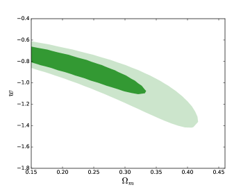
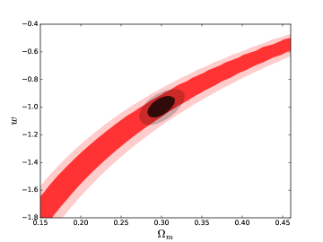
Figure 1: Confidence contours at 68% and 95% ($\Delta\chi^{2}=2.30$ and $\Delta\chi^{2}=6.17$, respectively) for the $\Omega_{m}$ and $w$ cosmological parameters of the $w$CDM model. Left panel: contours obtained using the SNIa and the BAO cosmological probes with $\omega_{b}=0.02262$ fixed. Right panel: the red (large) contours correspond to the CMB probe while the black (small) contours account for the combination of the three probes: SNIa, BAO and CMB.

In Fig. 1 we show the result of our analysis for the $w$CDM model, with the 1$\sigma$ and 2$\sigma$ contours obtained for the $\Omega_{m}$ and $w$ cosmological parameters. In the left panel only the information coming from the SNIa and the BAO probes has been used (fixing the reduced baryon density parameter to $\omega_{b}=0.02262$ Planck2015XIV ), while in the right panel the red contours correspond to the CMB probe and the black ones correspond to the combination of the three probes: SNIa+BAO+CMB. In these cases we have not fixed the baryon density as this quantity is well constrained by the CMB probe. We have marginalized over $H_{0}$ in both panels. The constraints we have obtained for the different models are summarized in Table 1. For the $w$CDM model, our constraints are (logically) very similar to those of Betoule2014 , whose authors used the BAO, SNIa and CMB through temperature fluctuations from Planck 2013 and polarization fluctuations from WMAP.

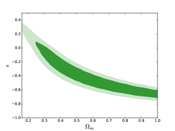
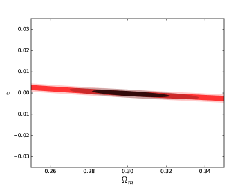
Figure 2: Confidence contours at 68% and 95% ($\Delta\chi^{2}=2.30$ and $\Delta\chi^{2}=6.17$, respectively) for the $\Omega_{m}$ and $\epsilon$ cosmological parameters of the $\epsilon$CDM model. Left panel: contours obtained using the SNIa and the BAO cosmological probes with $\omega_{b}=0.02262$ fixed. Right panel: the red (large) contours correspond to the CMB probe while the black (small) contours account for the combination of the three probes: SNIa, BAO and CMB.

In Fig. 2 the 1$\sigma$ and 2$\sigma$ contours for the $\Omega_{m}$ and $\epsilon$ parameters of the $\epsilon$CDM model are represented. As in Fig. 1, the left panel corresponds to the result using only SNIa+BAO (fixing $\omega_{b}=0.02262$), while the right panel shows the CMB contours and the combination of the three probes, with marginalization over the baryon density. We have marginalized over $H_{0}$ in all cases. The specific constraints we have obtained are $\Omega_{m}=0.301^{+0.014}_{-0.013}$ and $\epsilon=-0.0003\pm 0.0011$ (errors at 1$\sigma$ on one parameter), which clearly differ from the result in Avelino2012 , where they provide $\epsilon=0.009\pm 0.002$ at 3$\sigma$ confidence level. This difference can be due to the use of different cosmological probes. However, our results are compatible with Thomas2016 where the authors provide $\epsilon=0.00063^{+0.00108}_{-0.00112}$ at 2$\sigma$ confidence level, using Planck data plus lensing information and the BAO probe.

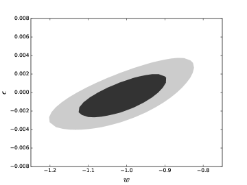
Figure 3: Confidence contours at 68% and 95% ($\Delta\chi^{2}=2.30$ and $\Delta\chi^{2}=6.17$, respectively) for the $w$ and $\epsilon$ cosmological parameters of the $\epsilon w$CDM model. The combination of the three probes SNIa, BAO and CMB has been used.

In Fig. 3 the 1$\sigma$ and 2$\sigma$ contours for the $w$ and $\epsilon$ cosmological parameters of the $\epsilon w$CDM model are provided. In this case only the combination of the three probes is represented, since the contours coming only from SNIa+BAO or only from the CMB are highly degenerated. We have marginalized over $H_{0}$ and $\omega_{b}$. The specific obtained constraints are $w=-1.010^{+0.075}_{-0.077}$ and $\epsilon=-0.0004\pm 0.0016$ (errors at 1$\sigma$ on one parameter), which are slightly worse than for the $w$CDM and $\epsilon$CDM models due to the introduction of a new degree of freedom.

All the constraints we have obtained are compatible with the standard $\Lambda$CDM model. However, it is important to stress two points here: first of all, we have seen the strong role of the CMB probe (SNIa+BAO alone cannot provide us with good constraints for the cosmological parameters) and, secondly, we have seen that the constraints on dark matter and dark energy are not completely independent (see Fig. 3). This implies that all the assumptions made in one of the sectors may influence the constraints obtained in the other one.

III DARK CONTENT(S) OF THE UNIVERSE: A EUCLID FORECAST

In this section we derive the expected precision achievable on the previous models, using the galaxy power spectrum Euclid survey in the linear regime.

III.1 Method

In the following, the forecast is based on a Fisher matrix formalism in a parametrized cosmological model considering the Hubble parameter and the angular-diameter distance as observables. We rely on the following matter power spectrum Amendola2013 :

$$P_{\text{matter}}(k,z)= \frac{8\pi^{2}c^{4}k_{0}\Delta_{R}^{2}(k_{0})}{25H_{0}^{4}\Omega_{m}^{2}}T^{2}(k)\cdot$$ (14)

$$\cdot\left[\frac{G(z)}{G(z=0)}\right]^{2}\left(\frac{k}{k_{0}}\right)^{n_{s}}\,,$$

where $G(z)$ is the growth function Carroll1992 ; Eisenstein1997 , $T(k)$ is the transfer function HS1996 ; Eisenstein1999 ; EHu1998 , $k_{0}=0.005$ Mpc^-1, $\Delta_{R}^{2}(k_{0})=2.22\times 10^{-9}$ Amendola2013 and $n_{s}=0.96$ Planck2015 is the spectral index. The observed galaxy power spectrum is different from the matter power spectrum because of the biasing of galaxies and their velocity field. It can be related to $P_{\text{matter}}$ by Seo2003

$$P_{\text{obs}}(k_{\perp},k_{\parallel},z)=\frac{D_{A}(z)^{2}_{\text{ref}}H(z)}{D_{A}(z)^{2}H(z)_{\text{ref}}}P_{g}(k_{\perp},k_{\parallel},z)+P_{\text{shot}}\,,$$ (15)

with

$$P_{g}(k_{\perp},k_{\parallel},z)=b(z)^{2}\left[1+\beta(z)\frac{k_{\parallel}^{2}}{k_{\parallel}^{2}+k_{\perp}^{2}}\right]P_{\text{matter}}(k,z)\,,$$ (16)

where $b(z)$ is the bias factor between the galaxy and matter distributions, $\beta(z)=f_{g}(z)/b(z)\approx\Omega_{m}^{0.6}/b(z)$ Seo2007 and $k_{\parallel},\,k_{\perp}$ stand for the parallel and transverse components of k. $P_{\text{shot}}$ is an unknown residual noise which we neglect, since it is expected to introduce negligible error Samushia2011 . The ref subscript stands for the reference cosmology.

For a given redshift interval, the Fisher matrix is given by Tegmark1997

$$F_{ij}= \int_{-1}^{1}\int_{k_{\text{min}}}^{k_{\text{max}}}\frac{\partial\ln P_{\text{obs}}(k,\mu)}{\partial p_{i}}\frac{\partial\ln P_{\text{obs}}(k,\mu)}{\partial p_{j}}\cdot$$ (17)

$$\cdot V_{\text{eff}}(k,\mu)\frac{2\pi k^{2}\,\text{d}k\,\text{d}\mu}{2(2\pi)^{3}}\,,$$

where we have changed $k_{\parallel},\,k_{\perp}$ by $k$ and $\mu$ (the modulus of k and the cosine of the angle between k and the line of sight, respectively). According to Seo2003 the maximum scale of the survey $k_{\text{min}}^{-1}$ has almost no effect on the results; therefore we adopt $k_{\text{min}}=0$. The minimum scale $k_{\text{max}}^{-1}$ is used to exclude scales affected by the nonlinear regime, where our linear power spectra would be inaccurate. We interpolate the values given in Seo2003 for $k_{\text{max}}$. The effective volume of the survey is given by

$$V_{\text{eff}}(k,\mu) =\int\left[\frac{n(\textbf{r})P(k,\mu)}{n(\textbf{r})P(k,\mu)+1}\right]^{2}\,\text{d}\textbf{r}$$ (18)

$$=\left[\frac{nP(k,\mu)}{nP(k,\mu)+1}\right]^{2}V_{\text{survey}}\,.$$

The last equality holds for a uniform density of galaxies. The comoving volume of the survey $V_{\text{survey}}$ is given by Hogg1999

$$V_{\text{survey}}=\int\text{d}\Omega\int_{z_{\text{min}}}^{z_{\text{max}}}\text{d}z\,\frac{c(1+z)^{2}D_{A}^{2}(z)}{H(z)}\,,$$ (19)

where $\Omega$ is the solid angle. According to Seo2003 we multiply the integrand of the Fisher matrix by an exponential suppression $e^{-k^{2}\mu^{2}\sigma_{r}^{2}}$, with $\sigma_{r}=c\sigma_{z}/H(z)$, in order to take into account the redshift error $\sigma_{z}$ of the galaxy survey. Once we have obtained the Fisher matrix for the observables $H(z)$ and $D_{A}(z)$ we can propagate it to the Fisher matrix for the parameters using Wang2010

$$F_{\alpha\alpha^{\prime}}=\sum_{ij}\frac{\partial p_{i}}{\partial q_{\alpha}}F_{ij}\frac{\partial p_{j}}{\partial q_{\alpha^{\prime}}}\,,$$ (20)

where $p_{i}$ stand for the observables $H(z)$ or $D_{A}(z)$, and $q_{\alpha}$ for the parameters under study. The Fisher matrix for all the redshift range of the survey is given by the sum of the Fisher matrices for each redshift bin. The inverse of the resulting Fisher matrix gives us the uncertainties and correlations of all the parameters studied in the forecast.

III.2 Euclid spectroscopic survey

In this work we focus our forecast on the typical results expected for the Euclid  space mission: an ESA medium class astronomy and astrophysics space mission which aims at understanding the accelerated expansion of the Universe and the nature of dark energy.

For simplicity, we restrict ourselves to the galaxy clustering probe of the Euclid mission. In order to adapt our forecast we only need five parameters, whose values are taken from the Euclid redbook Laureijs : the minimum and maximum redshift, $z_{\text{min}}=0.7$, $z_{\text{max}}=2.1$; the area, 15000 square degrees; the number of galaxies, $50\times 10^{6}$; and the precision of the redshift estimation, $\sigma_{z}/(1+z)\leq 0.1\%$. We adopt the bias given in Amendola2013 : $b(z)=\sqrt{1+z}$. We split the redshift range of the survey into bins of width 0.1 in redshift. Narrower bins only marginally increase the precision while requiring more computational time. Finally, the reference cosmology is the one obtained in Sec. II.3 and it is summarized in the fifth column of Table 1.

In this work we limit ourselves to the spectroscopic survey on linear scales. We have checked that the photometric survey only marginally improves the constraints on the parameters, while including weakly nonlinear scales noticeably improves these constraints. Combination with the weak lensing probe would obviously lead to even better constraints Majerotto2012 . A quantitative evaluation of these improvements is left for future work.

III.3 Results

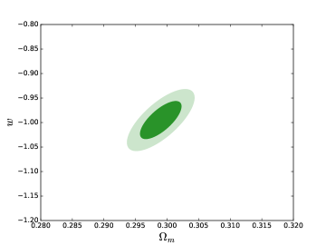
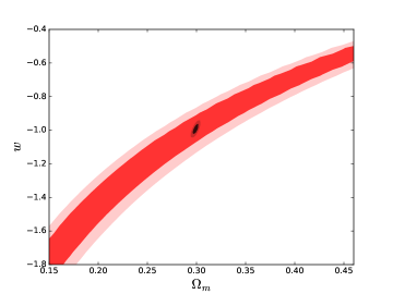
Figure 4: Confidence contours at 68% and 95% ($\Delta\chi^{2}=2.30$ and $\Delta\chi^{2}=6.17$, respectively) for the $\Omega_{m}$ and $w$ cosmological parameters of the $w$CDM model. Left panel: contours obtained using the Euclid galaxy clustering forecast with $\omega_{b}=0.02262$ fixed. Right panel: the red (large) contours correspond to the CMB probe while the black (small) contours account for the combination of the CMB and the Euclid galaxy clustering forecast.

The results for the $w$CDM model are represented in Fig. 4. In the left panel the 1$\sigma$ and 2$\sigma$ contours for the $\Omega_{m}$ and $w$ cosmological parameters are computed using the Euclid galaxy power spectrum forecast and fixing the reduced baryon density parameter to its reference value $\omega_{b}=0.02257$. In the right panel the red contours correspond to the CMB probe and the black contours stand for the combination of the CMB and the forecast assuming a Gaussian likelihood for the forecast. More precisely, when minimizing the $\chi^{2}$ function as presented in (4), we minimize the sum of the $\chi^{2}$ corresponding to the CMB plus a $\chi^{2}$ function associated to the forecast where the covariance matrix is directly the one provided by the forecast. We have marginalized over $H_{0}$ in all the figures. The results of the forecast are the following constraints: $\Omega_{m}=0.299\pm 0.022$ and $w=-0.995\pm 0.026$ (errors at 1$\sigma$ on one parameter), which are much better than the degeneracy obtained with SNIa+BAO present-day data (Fig. 1, left panel). Combination with the CMB gives $\Omega_{m}=0.2990\pm 0.0021$ and $w=-0.994\pm 0.022$ (errors at 1$\sigma$ on one parameter), which are between a factor 2 and 6 better than SNIa+BAO+CMB present-day data constraints (Fig. 1, right panel).

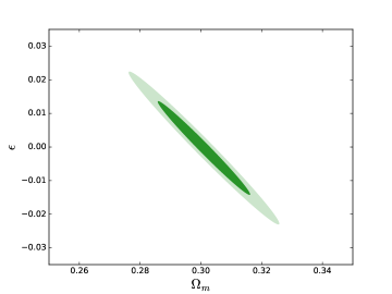
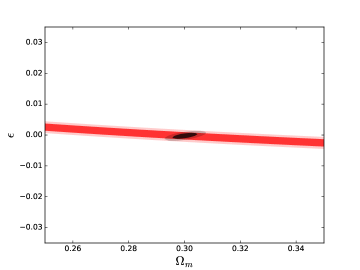
Figure 5: Confidence contours at 68% and 95% ($\Delta\chi^{2}=2.30$ and $\Delta\chi^{2}=6.17$, respectively) for the $\Omega_{m}$ and $\epsilon$ cosmological parameters of the $\epsilon$CDM model. Left panel: contours obtained using the Euclid galaxy clustering forecast with $\omega_{b}=0.02262$ fixed. Right panel: the red (large) contours correspond to the CMB probe while the black (small) contours account for the combination of the CMB and the Euclid galaxy clustering forecast.

The 1$\sigma$ and 2$\sigma$ contours for the $\Omega_{m}$ and $\epsilon$ cosmological parameters of the $\epsilon$CDM model are represented in Fig. 5. As in Fig. 4 the left panel corresponds to the Euclid galaxy power spectrum forecast with fixed baryon density, while the right panel corresponds to the CMB (red) and the combination of the forecast and the CMB (black) contours. We have also marginalized over $H_{0}$ in all the figures. The specific constraints given by the forecast are $\Omega_{m}=0.301\pm 0.010$ and $\epsilon=-0.0003\pm 0.0092$ (errors at 1$\sigma$ on one parameter), which again have greatly improved compared to the degeneracy found with SNIa+BAO present-day data (Fig. 2, left panel). Adding the CMB we obtain the constraints, $\Omega_{m}=0.3001\pm 0.0030$ and $\epsilon=-0.00024^{+0.00065}_{-0.00066}$ (errors at 1$\sigma$ on one parameter), which are between a factor 2 and 5 better than present-day SNIa+BAO+CMB constraints (Fig. 2, right panel).

Let us recall that all the results shown here are only for the galaxy clustering probe restricted to the linear scales, so we can expect significantly better constraints from the full exploitation of the future Euclid survey data.

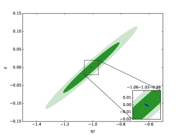
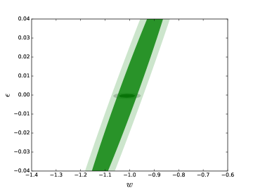
Figure 6: Confidence contours at 68% and 95% ($\Delta\chi^{2}=2.30$ and $\Delta\chi^{2}=6.17$, respectively) for the $\epsilon$ and $w$ cosmological parameters of the $\epsilon w$CDM model. Left panel: contours obtained using the Euclid galaxy clustering forecast with $\omega_{b}=0.02262$ fixed. In the small box on the lower right corner, the equivalent contours when fixing $H_{0}=68.6$ km s^-1 Mpc^-1 and $\Omega_{m}=0.301$ are represented. Right panel: the green (large) contours correspond to the forecast while the black (small) contours account for the combination with the CMB, marginalizing over the baryon density.

Figure 6 provides the 1$\sigma$ and 2$\sigma$ contours for the $w$ and $\epsilon$ cosmological parameters of the $\epsilon w$CDM model. The left panel corresponds to the forecast with fixed baryon density, while the right panel shows, in addition, the combination of the forecast with the CMB. We have marginalized over $H_{0}$ in both cases. The specific constraints we have obtained using the forecast are $w=-1.01\pm 0.13$ and $\epsilon=0.000\pm 0.046$ (errors at 1$\sigma$ on one parameter), which are much better than present-day SNIa+BAO degeneracies that do not provide any significant constraint (see the absence of constraints in the third column of Table 1). This is a remarkable result illustrating that Euclid can break this degeneracy in the dark sector at low redshift.

It is worth noticing, apart from the better constraints expected from the Euclid survey, that we still find  a significant correlation between the $\epsilon$ and $w$ cosmological parameters from the Euclid survey (Fig. 6, left panel, green contour) illustrating the fact that the dark matter and the dark energy sectors are not completely uncoupled and cannot be constrained independently from each other. However, the sign of this correlation may be somewhat surprising: if the total density were to be constant we would expect $w$ and $\epsilon$ to be anticorrelated. We have checked that this is indeed the case, when all the other parameters are kept fixed (see the small box in Fig. 6, left panel). When marginalizing over $H_{0}$ and $\Omega_{m}$ the correlation changes and leads to weak constraints on the dark energy equation of state parameter, $w=-1.01\pm 0.13$ ($w=-1.01$ being the fiducial value that corresponds to our best estimate in view of present-day constraints), and on the equation of state of dark matter $\epsilon=0\pm 0.046$.

Adding the CMB constraint to the forecast results in much more stringent limits on the parameters describing the dark sector, $w=-1.010\pm 0.023$ and $\epsilon=-0.00045^{+0.00065}_{-0.00066}$ (errors at 1$\sigma$ on one parameter), which are similar to the obtained constraints on the $w$CDM and the $\epsilon$CDM model parameters (Figs. 4 and 5, respectively). This fact highlights again the strong role of the CMB in breaking degeneracies thanks to the strong constraint on the dark matter equation of state parameter.

IV CONCLUSIONS

We have investigated consequences on cosmological constraints relaxing the pressureless nature of dark matter ($w_{DM}\neq 0$). We restricted ourselves to the simple case of constant equation of state parameter for both dark sectors. Even if not fully theoretically motivated, these simple models allow us to ascertain the maximum values that the equation of state parameters are allowed to take Kunz2016 . We have found that cosmological constraints from present-day SNIa and BAO data are strongly degraded, revealing a complete degeneracy between the equations of state of matter and dark energy. The constraints are essentially restored by the inclusion of CMB data thanks to its leverage. We have then studied the anticipated accuracy from the Euclid redshift galaxy survey. We have found that Euclid is expected to break the above degeneracy between dark matter and dark energy, but the high accuracy on the dark energy equation of state parameter is lost. Combining with the CMB allows us to restore constraints at a similar level to the $w_{DM}=0$ forecast in the specific model we investigated. We expect even better performance from the full exploitation of the future Euclid survey data, but the remaining correlation between dark matter and dark energy equation of state parameter deserves further investigation.

Table 1: Cosmological parameter constraints for the different models and the different probes considered (Euclid GC stands for the galaxy clustering probe of the Euclid survey). The errors are given at the 1$\sigma$ confidence level on one parameter ($\Delta\chi^{2}=1$). The $\Lambda$CDM model is included for comparison. The stars in some reduced baryon densities stand for fixed values. The dash in the $\epsilon w$CDM model using SNIa+BAO data stands for the extreme degeneracies which do not allow us to obtain significant constraints on the cosmological parameters.

		SNIa+BAO	Euclid GC	SNIa+BAO+CMB	Euclid GC + CMB
$\Lambda$CDM	$\Omega_{m}$	$0.288^{+0.032}_{-0.031}$	$0.2984^{+0.0015}_{-0.0015}$	$0.2984^{+0.0096}_{-0.0092}$	$0.2984^{+0.0015}_{-0.0015}$
	$H_{0}$	$67.6^{+2.7}_{-2.4}$	$68.80^{+0.10}_{-0.10}$	$68.80^{+0.75}_{-0.74}$	$68.80^{+0.10}_{-0.10}$
	$\omega_{b}$	$0.02262^{*}$	$0.02257^{*}$	$0.02257^{+0.00024}_{-0.00024}$	$0.022574^{+0.000098}_{-0.000098}$
$w$CDM	$\Omega_{m}$	$\leq 0.28$	$0.299^{+0.022}_{-0.022}$	$0.299^{+0.012}_{-0.011}$	$0.2990^{+0.0021}_{-0.0021}$
	$w$	$-0.72^{+0.18}_{-0.25}$	$-0.995^{+0.026}_{-0.026}$	$-0.995^{+0.052}_{-0.054}$	$-0.994^{+0.022}_{-0.022}$
	$H_{0}$	$53.0^{+13.3}_{-5.5}$	$68.70^{+0.45}_{-0.45}$	$68.7^{+1.3}_{-1.3}$	$68.68^{+0.39}_{-0.40}$
	$\omega_{b}$	$0.02262^{*}$	$0.02259^{*}$	$0.02259^{+0.00026}_{-0.00026}$	$0.022581^{+0.000098}_{-0.000098}$
$\epsilon$CDM	$\Omega_{m}$	$\geq 0.31$	$0.301^{+0.010}_{-0.010}$	$0.301^{+0.014}_{-0.013}$	$0.3001^{+0.0030}_{-0.0030}$
	$\epsilon$	$-0.49^{+0.44}_{-0.20}$	$-0.0003^{+0.0092}_{-0.0092}$	$-0.0003^{+0.0011}_{-0.0011}$	$-0.00024^{+0.00065}_{-0.00066}$
	$H_{0}$	$50.00^{+3.83}_{-0.90}$	$68.60^{+0.27}_{-0.27}$	$68.6^{+1.2}_{-1.2}$	$68.62^{+0.12}_{-0.12}$
	$\omega_{b}$	$0.02262^{*}$	$0.02262^{*}$	$0.02262^{+0.00029}_{-0.00029}$	$0.02262^{+0.00029}_{-0.00029}$
$\epsilon w$CDM	$\Omega_{m}$		$0.301^{+0.041}_{-0.041}$	$0.301^{+0.014}_{-0.013}$	$0.3011^{+0.0038}_{-0.0037}$
	$w$		$-1.01^{+0.13}_{-0.13}$	$-1.010^{+0.075}_{-0.077}$	$-1.010^{+0.023}_{-0.023}$
	$\epsilon$	$-$	$0.000^{+0.046}_{-0.046}$	$-0.0004^{+0.0016}_{-0.0016}$	$-0.00045^{+0.00065}_{-0.00066}$
	$H_{0}$		$68.6^{+1.0}_{-1.0}$	$68.6^{+1.3}_{-1.3}$	$68.60^{+0.44}_{-0.43}$
	$\omega_{b}$		$0.02262^{*}$	$0.02262^{+0.00029}_{-0.00029}$	$0.02262^{+0.00029}_{-0.00029}$

ACKNOWLEDGMENTS

We thank Stéphane Ilić for useful comments.

References

- (1) N. Aghanim, M. Arnaud, M. Ashdown et al. (Planck Collaboration), Planck 2015 results. XI. CMB power spectra, likelihoods, and robustness of parameters, Astron. Astrophys. 594, A11 (2016).
- (2) A. G. Riess, A. V. Filippenko, P. Challis et al., Observational Evidence from Supernovae for an Accelerating Universe and a Cosmological Constant, Astron. J. 116, 1009 (1998).
- (3) S. Perlmutter, G. Aldering, G. Goldhaber et al., Measurements of and from 42 High-Redshift Supernovae, Astrophys. J. 517, 565 (1999).
- (4) J. Martin, Everything you always wanted to know about the cosmological constant problem (but were afraid to ask), C.R. Phys. 13, 566 (2012).
- (5) R. R. Caldwell, R. Dave, and P. J. Steinhardt, Cosmological Imprint of an Energy Component with General Equation of State, Phys. Rev. Lett. 80, 1582 (1998).
- (6) S. Nojiri and S.D. Odintsov, Unified cosmic history in modified gravity: From F(R) theory to Lorentz non-invariant models, Phys. Rep. 505, 59 (2011).
- (7) T. Buchert, S. Räsänen, Backreaction in Late-Time Cosmology, Annu. Rev. Nucl. Part. Sci. 62, 57 (2012).
- (8) L. Amendola, S. Appleby, D. Bacon et al., Cosmology and fundamental physics with the Euclid satellite, Living Rev. Relativ. 16, 6 (2013).
- (9) W. Hu, Structure formation with generalized dark matter, Astrophys. J. 506, 485 (1998).
- (10) M. Kunz, Degeneracy between the dark components resulting from the fact that gravity only measures the total energy-momentum tensor, Phys. Rev. D 80, 123001 (2009).
- (11) E. Komatsu, K. M. Smith, J. Dunkley et al., Seven-year wilkinson microwave anisotropy probe (WMAP *) observations: cosmological interpretation, Astrophys. J. Suppl. Ser. 192, 18 (2011).
- (12) M. Betoule, R. Kessler, J. Guy et al., Improved cosmological constraints from a joint analysis of the SDSS-II and SNLS supernova samples, Astron. Astrophys. 568, A22 (2014).
- (13) M. Sako, B. Bassett, A. C. Becker et al., The Data Release of the Sloan Digital Sky Survey-II Supernova Survey, arXiv:1401.3317.
- (14) A. Conley, J. Guy, M. Sullivan et al., Supernova constraints and systematic uncertainties from the first three years of the supernova legacy survey, Astrophys. J. Suppl. Ser. 192, 1 (2011).
- (15) F. Beutler, C. Blake, M. Colless, D. H. Jones, L. Staveley-Smith, L. Campbell, Q. Parker, W. Saunders, and F. Watson, The 6dF Galaxy Survey: baryon acoustic oscillations and the local Hubble constant, Mon. Not. R. Astron. Soc. 416, 3017 (2011).
- (16) N. Padmanabhan, X. Xu, D. J. Eisenstein, R. Scalzo, A. J. Cuesta, K. T. Mehta, and E. Kazin, A 2 per cent distance to by reconstructing baryon acoustic oscillations – I. Methods and application to the Sloan Digital Sky Survey, Mon. Not. R. Astron. Soc. 427, 2132 (2012).
- (17) L. Anderson, E. Aubourg, S. Bailey et al., The clustering of galaxies in the SDSS-III Baryon Oscillation Spectroscopic Survey: baryon acoustic oscillations in the Data Release 9 spectroscopic galaxy sample, Mon. Not. R. Astron. Soc. 427, 3435 (2012).
- (18) P. A. R. Ade, N. Aghanim, C. Armitage-Caplan et al. (Planck Collaboration), Planck 2013 results. XVI. Cosmological parameters, Astron. Astrophys. 571, A16 (2014).
- (19) D. J. Eisenstein and W. Hu, Baryonic features in the matter transfer function, Astrophys. J. 496, 605 (1998).
- (20) Y. Wang and P. Mukherjee, Observational constraints on dark energy and cosmic curvature, Phys. Rev. D 76, 103533 (2007).
- (21) W. Hu and N. Sugiyama, Small-scale cosmological perturbations: an analytic approach, Astrophys. J. 471, 542 (1996).
- (22) P. A. R. Ade, N. Aghanim, M. Arnaud et al. (Planck Collaboration), Planck 2015 results. XIV. Dark energy and modified gravity, Astron. Astrophys. 594, A14 (2016).
- (23) C. Cheng and Q. G. Huang, Dark side of the Universe after Planck data, Phys. Rev. D 89, 043003 (2014).
- (24) D. B. Thomas, M. Kopp, and C. Skordis, Constraining the properties of dark matter with observations of the cosmic microwave background, Astrophys. J. 830, 155 (2016).
- (25) F. James and M. Roos, Minuit - a system for function minimization and analysis of the parameter errors and correlations, Comput. Phys. Commun. 10, 343 (1975).
- (26) F. Couchot, S. Henrot-Versillé, O. Perdereau, S. Plaszczynski, B. Rouillé d’Orfeuil, M. Spinelli, and M. Tristram, Relieving tensions related to the lensing of CMB temperature power spectra, arXiv:1510.07600 [Astron. Astrophys. (to be published)].
- (27) P. A. R. Ade, N. Aghanim, M. Arnaud et al. (Planck Collaboration), Planck intermediate results. XVI. Profile likelihoods for cosmological parameters, Astron. Astrophys. 566, A54 (2014).
- (28) A. Avelino, N. Cruz, and U. Nucamendi, Testing the EoS of dark matter with cosmological observations, arXiv:1211.4633.
- (29) S. M. Carroll, W. H. Press, and E. L. Turner, The cosmological constant, Annu. Rev. Astron. Astrophys. 30, 499 (1992).
- (30) D.J. Eisenstein, An Analytic expression for the growth function in a flat universe with a cosmological constant, arXiv:astro-ph/9709054.
- (31) D. J. Eisenstein and W. Hu, Power spectra for cold dark matter and its variants, Astrophys. J. 511, 5 (1999).
- (32) H. Seo and D.J. Eisenstein, Probing dark energy with baryonic acoustic oscillations from future large galaxy redshift surveys, Astrophys. J. 598, 720 (2003).
- (33) H. Seo and D.J. Eisenstein, Improved forecasts for the baryon acoustic oscillations and cosmological distance scale, Astrophys. J. 665, 14 (2007).
- (34) L. Samushia, W.J. Percival, L. Guzzo et al., Effects of cosmological model assumptions on galaxy redshift survey measurements, Mon. Not. R. Astron. Soc. 410, 1993 (2011).
- (35) M. Tegmark, Measuring Cosmological Parameters with Galaxy Surveys, Phys. Rev. Lett. 79, 3806 (1997).
- (36) D. W. Hogg, Distance measures in cosmology, arXiv:astro-ph/9905116.
- (37) Y. Wang, W. Percival, A. Cimatti et al., Designing a space-based galaxy redshift survey to probe dark energy, Mon. Not. R. Astron. Soc. 409, 737 (2010).
- (38) R. Laureijs, J. Amiaux, S. Arduini et al., Euclid definition study report, arXiv:1110.3193.
- (39) E. Majerotto, L. Guzzo, L. Samushia et al., Probing deviations from general relativity with the Euclid spectroscopic survey, Mon. Not. R. Astron. Soc. 424, 1392 (2012).
- (40) M. Kunz, S. Nesseris, and I. Sawicki, Constraints on dark-matter properties from large-scale structure, Phys. Rev. D 94, 023510 (2016).