Learning of Generalized Low-Rank Models: A Greedy Approach

Abstract

Learning of low-rank matrices is fundamental to many machine learning applications. A state-of-the-art algorithm is the rank-one matrix pursuit (R1MP). However, it can only be used in matrix completion problems with the square loss. In this paper, we develop a more flexible greedy algorithm for generalized low-rank models whose optimization objective can be smooth or nonsmooth, general convex or strongly convex. The proposed algorithm has low per-iteration time complexity and fast convergence rate. Experimental results show that it is much faster than the state-of-the-art, with comparable or even better prediction performance.

1 Introduction

In many machine learning problems, the data samples can be naturally represented as low-rank matrices. For example, in recommender systems, the ratings matrix is low-rank as users (and items) tend to form groups. The prediction of unknown ratings is then a low-rank matrix completion problem Candès and Recht (2009). In social network analysis, the network can be represented by a matrix with entries representing similarities between node pairs. Unknown links are treated as missing values and predicted as in matrix completion Chiang et al. (2014). Low-rank matrix learning also have applications in image and video processing Candès et al. (2011), multitask learning Argyriou et al. (2006), multilabel learning Tai and Lin (2012), and robust matrix factorization Eriksson and van den Hengel (2012).

The low-rank matrix optimization problem is NP-hard Recht et al. (2010), and direct minimization is difficult. To alleviate this problem, one common approach is to factorize the target $m\times n$ matrix $X$ as a product of two low-rank matrices $U$ and $V$, where $U\in\mathbb{R}^{m\times r}$ and $V\in\mathbb{R}^{n\times r}$ with $r\ll\min\{m,n\}$. Gradient descent and alternating minimization are often used for optimization Srebro et al. (2004); Eriksson and van den Hengel (2012); Wen et al. (2012). However, as the objective is not jointly convex in $U$ and $V$, this approach can suffer from slow convergence Hsieh and Olsen (2014).

Another approach is to replace the matrix rank by the nuclear norm (i.e., sum of its singular values). It is known that the nuclear norm is the tightest convex envelope of the matrix rank Candès and Recht (2009). The resulting optimization problem is convex, and popular convex optimization solvers such as the proximal gradient algorithm Beck and Teboulle (2009) and Frank-Wolfe algorithm Jaggi (2013) can be used. However, though convergence properties can be guaranteed, singular value decomposition (SVD) is required in each iteration to generate the next iterate. This can be prohibitively expensive when the target matrix is large. Moreover, nuclear norm regularization often leads to biased estimation. Compared to factorization approaches, the obtained rank can be much higher and the prediction performance is inferior Mazumder et al. (2010).

Recently, greedy algorithms have been explored for low-rank optimization Shalev-shwartz et al. (2011a); Wang et al. (2014). The idea is similar to orthogonal matching pursuit (OMP) Pati et al. (1993) in sparse coding. For example, the state-of-the-art in matrix completion is the rank-one matrix pursuit (R1MP) algorithm Wang et al. (2014). In each iteration, it performs an efficient rank-one SVD on a sparse matrix, and then greedily adds a rank-one matrix to the matrix estimate. Unlike other algorithms which typically require a lot of iterations, it only takes $r$ iterations to obtain a rank-$r$ solution. Its prediction performance is also comparable or even better than others.

However, R1MP is only designed for matrix completion with the square loss. As recently discussed in Udell et al. (2015), different loss functions may be required in different learning scenarios. For example, in link prediction, the presence or absence of a link is naturally represented by a binary variable, and the logistic loss is thus more appropriate. In robust matrix learning applications, the $\ell_{1}$ loss or Huber loss can be used to reduce sensitivity to outliers Candès et al. (2011). While computationally R1MP can be used with these loss functions, its convergence analysis is tightly based on OMP (and thus the square loss), and cannot be easily extended.

This motivates us to develop more general greedy algorithms that can be used in a wider range of low-rank matrix learning scenarios. In particular, we consider low-rank matrix optimization problems of the form

$$\min_{X}f(X)\;:\;\text{rank}(X)\leq r,$$ (1)

where $r$ is the target rank, and the objective $f$ can be smooth or nonsmooth, (general) convex or strongly convex. The proposed algorithm is an extension of R1MP, and can be reduced to R1MP when $f$ is the square loss. In general, when $f$ is convex and Lipschitz-smooth, convergence is guaranteed with a rate of $O(1/T)$. When $f$ is strongly convex, this is improved to a linear rate. When $f$ is nonsmooth, we obtain a $O(1/\sqrt{T})$ rate for (general) convex objectives and $O(\log(T)/T)$ for strongly convex objectives. Experiments on large-scale data sets demonstrate that the proposed algorithms are much faster than the state-of-the-art, while achieving comparable or even better prediction performance.

Notation: The transpose of vector / matrix is denoted by the superscript $\ {}^{\top}$. For matrix $A=[A_{ij}]\in\mathbb{R}^{m\times n}$ (without loss of generality, we assume that $m\leq n$), its Frobenius norm is $\|A\|_{F}=\sqrt{\sum_{i,j}A_{ij}^{2}}$, $\ell_{1}$ norm is $||X||_{1}=\sum_{i,j}|X_{ij}|$, nuclear norm is $\|A\|_{*}=\sum_{i}\sigma_{i}(A)$, where $\sigma_{i}(A)$’s are the singular values, and $\sigma_{\max}(A)$ is its largest singular value. For two vectors $x,y$, the inner product $\langle x,y\rangle=\sum_{i}x_{i}y_{i}$; whereas for two matrices $A$ and $B$, $\langle A,B\rangle=\sum_{i,j}A_{ij}B_{ij}$. For a smooth function $f$, $\nabla f$ denotes its gradient. When $f$ is convex but nonsmooth, $g\in\{u\,|\,f(y)\geq f(x)+\langle u,x-y\rangle\}$ is its subgradient at $x$. Moreover, given $\Omega\in\{0,1\}^{m\times n}$, $[P_{\Omega}(A)]_{ij}=A_{ij}$ if $\Omega_{ij}=1$, and 0 otherwise.

2 Review: Rank-One Matrix Pursuit

The rank-one matrix pursuit (R1MP) algorithm Wang et al. (2014) is designed for matrix completion Candès and Recht (2009). Given a partially observed $m\times n$ matrix $O=[O_{ij}]$, indices of the observed entries are contained in the matrix $\Omega\in\{0,1\}^{m\times n}$, where $\Omega_{ij}=1$ if $O_{ij}$ is observed and 0 otherwise. The goal is to find a low-rank matrix that is most similar to $O$ at the observed entries. Mathematically, this is formulated as the following optimization problem:

$$\min_{X}\sum_{(i,j)\in\Omega}(X_{ij}-O_{ij})^{2}\;:\;\text{rank}(X)\leq r,$$ (2)

where $r$ is the target rank. Note that the square loss has to be used in R1MP.

The key observation is that if $X$ has rank $r$, it can be written as the sum of $r$ rank-one matrices, i.e., $X=\sum_{i=1}^{r}\theta_{i}u_{i}v_{i}^{\top}$, where $\theta_{i}\in\mathbb{R}$ and $\left\|u_{i}\right\|_{2}=\left\|v_{i}\right\|_{2}=1$. To solve (2), R1MP starts with an empty estimate. At the $t$th iteration, the $(u_{t},v_{t})$ pair that is most correlated with the current residual $R_{t}=P_{\Omega}(O-X_{t-1})$ is greedily added. It can be easily shown that this $(u_{t},v_{t})$ pair are the leading left and right singular vectors of $R_{t}$, and can be efficiently obtained from the rank-one SVD of $R_{t}$. After adding this new $u_{t}v_{t}^{\top}$ basis matrix, all coefficients of the current basis can be updated as

$$\!\!(\theta_{1},\dots,\theta_{t})\leftarrow\arg\min_{\theta_{1},\dots,\theta_{t}}\;\left\|P_{\Omega}\left(\sum_{i=1}^{t}\theta_{i}u_{i}v_{i}^{\top}-O\right)\right\|_{F}^{2}\!\!\!.\!\!\!$$ (3)

Because of the use of the square loss, this is a simple least-squares regression problem with closed-form solution.

To save computation, R1MP also has an economic variant. This only updates the combination coefficients of the current estimate and the rank-one update matrix as:

$$\!\!\!(\mu,\rho)\!\leftarrow\!\arg\min_{\mu,\rho}\;\left\|P_{\Omega}\left(\mu\sum_{i=1}^{t-1}\theta_{i}u_{i}v_{i}^{\top}\!+\!\rho u_{t}v_{t}^{\top}\!-\!O\right)\right\|_{F}^{2}\!\!\!.$$ (4)

The whole procedure is shown in Algorithm 1.

Algorithm 1 R1MP Wang et al. (2014).

1:  Initialize: $X_{0}=0$;

2:  for $t=1,\dots,T$ do

3:     $R_{t}=P_{\Omega}(O-X_{t-1})$;

4:     $[u_{t},s_{t},v_{t}]=\text{rank1SVD}(R_{t})$;

5:     update coefficients using (3) (standard version), or (4) (economic version);

6:     $X_{t}=\sum_{i=1}^{t}\theta_{i}u_{i}v_{i}^{\top}$;

7:  end for

8:  return  $X_{T}$.

Note that each R1MP iteration is computationally inexpensive. Moreover, as the matrix’s rank is increased by one in each iteration, only $r$ iterations are needed in order to obtain a rank-$r$ solution. It can also be shown that the residual’s norm decreases at a linear rate, i.e., $\|R_{t}\|_{F}^{2}\leq\gamma^{t-1}\|P_{\Omega}(O)\|_{F}^{2}$ for some $\gamma\in(0,1)$.

3 Low-Rank Matrix Learning with Smooth Objectives

Though R1MP is scalable, it can only be used for matrix completion with the square loss. In this Section, we extend R1MP to problems with more general, smooth objectives. Specifically, we only assume that the objective $f$ is convex and $L$-Lipschitz smooth. This will be further extended to nonsmooth objectives in Section 4.

Definition 1.

$f$ is $L$-Lipschitz smooth if $f(X)\leq f(Y)+\left\langle X-Y,\nabla f(Y)\right\rangle+\frac{L}{2}\|X-Y\|_{F}^{2}$ for any $X,Y$.

3.1 Proposed Algorithm

Let the matrix iterate at the $t$th iteration be $X_{t-1}$. We follow the gradient direction $\nabla f(X_{t-1})$ of the objective $f$, and find the rank-one matrix $M$ that is most correlated with $\nabla f(X_{t-1})$:

$$\max_{M}\;\langle M,\nabla f(X_{t-1})\rangle\;:\;\text{rank}(M)=1,\|M\|_{F}=1.$$ (5)

Similar to Wang et al. (2014), its optimal solution is given by $u_{t}v_{t}^{\top}$, where $(u_{t},v_{t})$ are the leading left and right singular vectors of $\nabla f(X_{t-1})$. We then set the coefficient $\theta_{t}$ for this new rank-one update matrix to $-s_{t}/L$, where $s_{t}$ is the singular value corresponding to $(u_{t},v_{t})$. Optionally, all the coefficients $\theta_{1},\dots,\theta_{t}$ can be refined as

$$(\theta_{1},\dots,\theta_{t})\leftarrow\arg\min_{\theta_{1},\dots,\theta_{t}}\;f\left(\sum_{i=1}^{t}\theta_{i}u_{i}v_{i}^{\top}\right).$$ (6)

As in R1MP, an economic variant is to update the coefficients as $[\mu\theta_{1},\dots,\mu\theta_{t-1},\rho]$, where $\mu$ and $\rho$ are obtained as

$$(\mu,\rho)\leftarrow\arg\min_{\mu,\rho}\;f\left(\mu\sum_{i=1}^{t-1}\theta_{i}u_{i}v_{i}^{\top}+\rho\,u_{t}v_{t}^{\top}\right).$$ (7)

The whole procedure, which will be called “greedy low-rank learning” (GLRL), is shown in Algorithm 2. Its economic variant will be called EGLRL. Obviously, on matrix completion problems with the square loss, Algorithm 2 reduces to R1MP.

Algorithm 2 GLRL for low-rank matrix learning with smooth convex objective $f$.

1:  Initialize: $X_{0}=0$;

2:  for $t=1,\dots,T$ do

3:     $[u_{t},s_{t},v_{t}]=\text{rank1SVD}(\nabla f(X_{t-1}))$;

4:     $X_{t}=X_{t-1}-\frac{s_{t}}{L}u_{t}v_{t}^{\top}$;

5:     (optional:) refine coefficients using (6) (standard version) or (7) (economic version);

6:  end for

7:  return  $X_{T}$.

Note that (6), (7) are smooth minimization problems (with $\leq r$ and 2 variables, respectively). As the target matrix is low-rank, $r$ should be small and thus (6), (7) can be solved inexpensively. In the experiments, we use the popular limited-memory BGFS (L-BFGS) solver Nocedal and Wright (2006). Empirically, fewer than five L-BFGS iterations are needed. Preliminary experiments show that using more iterations does not improve performance.

Unlike R1MP, note that the coefficient refinement at step 5 is optional. Convergence results in Theorems 2 and 3 below still hold even when this step is not performed. However, as will be illustrated in Section 5.1, coefficient refinement is always beneficial in practice. It results in a larger reduction of the objective in each iteration, and thus a better rank-$r$ model after running for $r$ iterations.

3.2 Convergence

The analysis of R1MP is based on orthogonal matching pursuit Pati et al. (1993). This requires the condition $\frac{1}{2}\|\nabla f(X)\|_{F}^{2}=f(X)$, which only holds when $f$ is the square loss. In contrast, our analysis for Algorithm 2 here is novel and can be used for any Lipschitz-smooth $f$.

The following Proposition shows that the objective is decreasing in each iteration. Because of the lack of space, all the proofs will be omitted.

Proposition 1.

If $f$ is $L$-Lipschitz smooth,

$$f(X_{t})\leq f(X_{t-1})-\frac{\gamma_{t-1}^{2}}{2L}\|\nabla f(X_{t-1})\|_{F}^{2},$$

where

$$\gamma_{t-1}=\frac{\sigma_{\max}(\nabla f(X_{t-1}))}{\|\nabla f(X_{t-1})\|_{F}}\in\left[\frac{1}{\sqrt{m}},1\right].$$ (8)

If $f$ is strongly convex, a linear convergence rate can be obtained.

Definition 2.

$f$ is $\mu$-strongly convex if $f(X)\geq f(Y)+\left\langle X-Y,\nabla f(Y)\right\rangle+\frac{\mu}{2}\|X-Y\|_{F}^{2}$ for any $X,Y$.

Theorem 2.

Let $X_{*}$ be the optimal solution of (1). If $f$ is $\mu$-strongly convex and $L$-Lipschitz smooth, then

$$f(X_{T})-f(X_{*})\leq\left(1-\frac{d_{1}^{2}\mu}{L}\right)^{T}\left[f(X_{0})-f(X_{*})\right],$$

where $d_{1}=\min_{t=1}^{T}\gamma_{t}$.

If $f$ is only (general) convex, the following shows that Algorithm 2 converges at a slower $O(1/T)$ rate.

Theorem 3.

If $f$ is (general) convex and $L$-Lipschitz smooth, then

$$f(X_{T})-f(X_{*})\leq\frac{2d_{2}^{2}L\left[f(X_{0})-f(X_{*})\right]}{d_{1}^{2}T\left[f(X_{0})-f(X_{*})\right]+2d_{2}^{2}L},$$

where $d_{2}=\max_{t=1}^{T}\|X_{t}-X_{*}\|_{F}$.

The square loss in (2) is only general convex and $1$-Lipschitz smooth. From Theorem 3, one would expect GLRL to only have a sublinear convergence rate of $O(1/T)$ on matrix completion problems. However, our analysis can be refined in this special case. The following Theorem shows that a linear rate can indeed be obtained, which also agrees with Theorem 3.1 of Wang et al. (2014).

Theorem 4.

When $f$ is the square loss, $f(X_{T})-f(X_{*})\leq(1-d_{1}^{2})^{T}\left[f(X_{0})-f(X_{*})\right]$.

3.3 Per-Iteration Time Complexity

The per-iteration time complexity of Algorithm 2 is low. Here, we take the link prediction problem in Section 5.1 as an example. With $f$ defined only on the observed entries of the link matrix, $\nabla f$ is sparse, and computation of $\nabla f(X_{t-1})$ in step 3 takes $O(||\Omega||_{1})$ time. The rank-one SVD on $\nabla f(X_{t-1})$ can be obtained by the power method Halko et al. (2011) in $O(||\Omega||_{1})$ time. Refining coefficients using (6) takes $O(t||\Omega||_{1})$ time for the $t$th iteration. Thus, the total per-iteration time complexity of GLRL is $O(t||\Omega||_{1})$. Similarly, the per-iteration time complexity of EGLRL is $O(||\Omega||_{1})$. In comparison, the state-of-the-art AIS-Impute algorithm Yao and Kwok (2015) (with a convergence rate of $O(1/T^{2})$) takes $O(r^{2}||\Omega||_{1})$ time in each iteration, whereas the alternating minimization approach in Chiang et al. (2014) (whose convergence rate is unknown) takes $O(r||\Omega||_{1})$ time per iteration.

3.4 Discussion

To learn the generalized low-rank model, Udell et al. (2015) followed the common approach of factorizing the target matrix as a product of two low-rank matrices and then performing alternating minimization Srebro et al. (2004); Eriksson and van den Hengel (2012); Wen et al. (2012); Chiang et al. (2014); Yu et al. (2014). However, this may not be very efficient, and is much slower than R1MP on matrix completion problems Wang et al. (2014). More empirical comparisons will be demonstrated in Section 5.1.

Similar to R1MP, the greedy efficient component optimization (GECO) Shalev-shwartz et al. (2011a) is also based on greedy approximation but can be used with any smooth objective. However, GECO is even slower than R1MP Wang et al. (2014). Moreover, it does not have convergence guarantee.

4 Low-Rank Matrix Learning with Nonsmooth Objectives

Depending on the application, different (convex) nonsmooth loss functions may be used in generalized low-rank matrix models Udell et al. (2015). For example, the $\ell_{1}$ loss is useful in robust matrix factorization Candès et al. (2011), the scalene loss in quantile regression Koenker (2005), and the hinge loss in multilabel learning Yu et al. (2014). In this Section, we extend the GLRL algorithm, with simple modifications, to nonsmooth objectives.

4.1 Proposed Algorithm

As the objective is nonsmooth, one has to use the subgradient $g_{t}$ of $f(X_{t-1})$ at the $t$th iteration instead of the gradient in Section 3. Moreover, refining the coefficients as in (6) or (7) will now involve nonsmooth optimization, which is much harder. Hence, we do not optimize the coefficients. To ensure convergence, a sufficient reduction in the objective in each iteration is still required. To achieve this, instead of just adding a rank-one matrix, we add a rank-$k$ matrix (where $k$ may be greater than 1). This matrix should be most similar to $g_{t}$, which can be easily obtained as:

$$M^{*}\equiv\arg\min_{M:\text{rank}(M)=k}\|M-g_{t}\|_{F}^{2}=\sum_{i=1}^{k}s_{i}u_{i}v_{i}^{\top},$$ (9)

where $\{(u_{1},v_{1}),\dots,(u_{k},v_{k})\}$ are the $k$ leading left and right singular vectors of $g_{t}$, and $\{s_{1},\dots,s_{k}\}$ are corresponding singular values. The proposed procedure is shown in Algorithm 3. The stepsize in step 3 is given by

$$\eta_{t}=\left\{\begin{array}[]{ll}c_{1}/t&\text{if $f$ is $\mu$-strongly convex}\\ c_{2}/\sqrt{t}&\text{if $f$ is (general) convex}\end{array}\right.,$$ (10)

where $c_{1}\geq 1/\mu$ and $c_{2}>0$.

Algorithm 3 GLRL for low-rank matrix learning with nonsmooth objective $f$.

1:  Initialize: $X_{0}=0$ and choose $\nu\in\left(0,1\right)$;

2:  for $t=1,\dots,T$ do

3:     set $\eta_{t}$ as in (10);

4:     compute subgradient $g_{t}$ of $f(X_{t-1})$, $h_{t}=0$;

5:     for $i=1,2,\dots$ do

6:        $[u_{i},s_{i},v_{i}]=\text{rank1SVD}(g_{t}-h_{t})$;

7:        $h_{t}=h_{t}+s_{i}u_{i}v_{i}^{\top}$;

8:        if $\|g_{t}-h_{t}\|_{F}^{2}\leq\nu\|g_{t-1}-h_{t-1}\|_{F}^{2}$ then

9:           break;

10:        end if

11:     end for

12:     $X_{t}=X_{t-1}-\eta_{t}h_{t}$;

13:  end for

14:  return  $X_{T}$.

4.2 Convergence

The following Theorem shows that when $f$ is nonsmooth and strongly convex, Algorithm 3 has a convergence rate of $O(\log{T}/T)$.

Theorem 5.

Assume that $f$ is $\mu$-strongly convex, and $\|g_{t}\|_{F}\leq b_{1}$ for some $b_{1}$ ($t=1,\dots,T$), then

$$\min_{t=0,\dots,T}f(X_{t})-f(X_{*})\leq\frac{1}{T}\left(\left(1+\log T\right)\frac{c_{1}b_{1}^{2}}{2}+b_{2}\right),$$

where $c_{1}$ is as defined in (10), and $b_{2}$ is a constant (depending on $X_{0}$, $\mu$, $\nu$ and $c_{1}$).

When $f$ is only (general) convex, the following Theorem shows that the rate is reduced to $O(1/\sqrt{T})$.

Theorem 6.

Assume that $f$ is (general) convex, $\|g_{t}\|_{F}\leq b_{1}$ for some $b_{1}$ and $\|X_{t}-X_{*}\|_{F}\leq b_{3}$ for some $b_{3}$ ($t=1,\dots,T$), then

$$\min_{t=0,\dots,T}f(X_{t})-f(X_{*})\leq\frac{c_{2}(b_{1}^{2}+b_{3}^{2})}{2\sqrt{T}}-\frac{2b_{1}b_{3}}{(1-\sqrt{\nu})T},$$

where $c_{2}$ is as defined in (10).

For other convex nonsmooth optimization problems, the same $O(\log(T)/T)$ rate for strongly convex objectives and and $O(1/\sqrt{T})$ rate for general convex objectives have also been observed Shalev-Shwartz et al. (2011b). However, their analysis is for different problems, and cannot be readily applied to our low-rank matrix learning problem here.

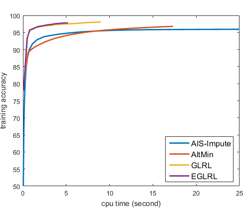
(a) Epinions (training).

(b) Epinions (testing).

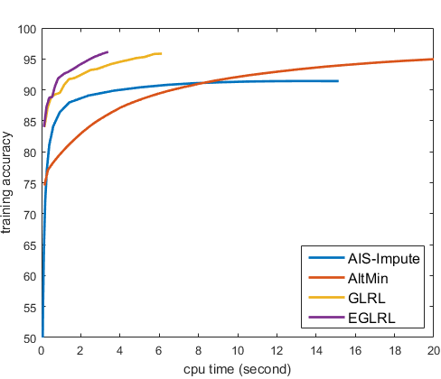
(c) Slashdot (training).

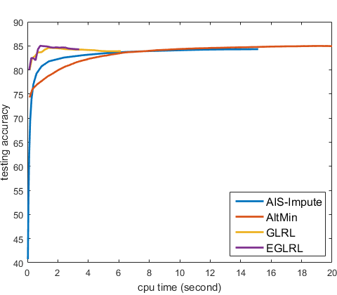
(d) Slashdot (testing).

Figure 1: Training and testing accuracies (%) vs CPU time (seconds) on the Epinions (left) and Slashdot (right) data sets.

4.3 Per-Iteration Time Complexity

To study the per-iteration time complexity, we take the robust matrix factorization problem in Section 5.2 as an example. The main computations are on steps 4 and 6. In step 4, since the subgradient $g_{t}$ is sparse (nonzero only at the observed entries), computing $g_{t}$ takes $O(||\Omega||_{1})$ time. At outer iteration $t$ and inner iteration $i$, $g_{t}$ in step 6 is sparse and $h_{t}$ has low rank (equal to $i-1$). Thus, $g_{t}-h_{t}$ admits the so-called “sparse plus low-rank” structure Mazumder et al. (2010); Yao et al. (2015). This allows matrix-vector multiplications and subsequently rank-one SVD to be performed much more efficiently. Specifically, for any $v\in\mathbb{R}^{n}$, the multiplication $(g_{t}-h_{t})v$ takes only $O(||\Omega||_{1}+(i-1)n)$ time (and similarly for the multiplication $u^{\top}(g_{t}-h_{t})$ with any $u\in\mathbb{R}^{m}$), and rank-one SVD using the power method takes $O(||\Omega||_{1}+(i-1)n)$ time. Assuming that $i_{t}$ inner iterations are run at (outer) iteration $t$, it takes a total of $O(i_{t}||\Omega||_{1}+(i_{t}-1)^{2}n)$ time. Typically, $i_{t}$ is small (empirically, usually 1 or 2).

In comparison, though the ADMM algorithm in Lin et al. (2010) has a faster $O(1/T)$ convergence rate, it needs SVD and takes $O(m^{2}n)$ time in each iteration. As for the Wiberg algorithm Eriksson and van den Hengel (2012), its convergence rate is unknown and a linear program with $mr+||\Omega||_{1}$ variables needs to be solved in each iteration. As will be seen in Section 5.2, this is much slower than GLRL.

5 Experiments

In this section, we compare the proposed algorithms with the state-of-the-art on link prediction and robust matrix factorization. Experiments are performed on a PC with Intel i7 CPU and 32GB RAM. All the codes are in Matlab.

5.1 Social Network Analysis

Given a graph with $m$ nodes and an incomplete adjacency matrix $O\in\{\pm 1\}^{m\times m}$, link prediction aims to recover a low-rank matrix $X\in\mathbb{R}^{m\times m}$ such that the signs of $X_{ij}$’s and $O_{ij}$’s agree on most of the observed entries. This can be formulated as the following optimization problem Chiang et al. (2014):

$$\min_{X}\sum_{(i,j)\in\Omega}\log(1+\exp(-X_{ij}O_{ij}))\;:\;\text{rank}(X)\leq r,$$ (11)

where $\Omega$ contains indices of the observed entries. Note that (11) uses the logistic loss, which is more appropriate as $O_{ij}$’s are binary.

The objective in (11) is convex and smooth. Hence, we compare the proposed GLRL (Algorithm 2 with coefficient update step (6)) and its economic variant EGLRL (using coefficient update step (7)) with the following:

1. AIS-Impute Yao and Kwok (2015): This is an accelerated proximal gradient algorithm with further speedup based on approximate SVD and the special “sparse plus low-rank” matrix structure in matrix completion;

2. Alternating minimization (“AltMin”) Chiang et al. (2014): This factorizes $X$ as a product of two low-rank matrices, and then uses alternating gradient descent for optimization.

As a further baseline, we also compare with the GLRL variant that does not perform coefficient update. We do not compare with greedy efficient component optimization (GECO) Shalev-shwartz et al. (2011a), matrix norm boosting Zhang et al. (2012) and active subspace selection Hsieh and Olsen (2014), as they have been shown to be slower than AIS-Impute and AltMin Yao and Kwok (2015); Wang et al. (2014).

Experiments are performed on the Epinions and Slashdot data sets Chiang et al. (2014) (Table 1). Each row/column of the matrix $O$ corresponds to a user (users with fewer than two observations are removed). For Epinions, $O_{ij}=1$ if user $i$ trusts user $j$, and $-1$ otherwise. Similarly for Slashdot, $O_{ij}=1$ if user $i$ tags user $j$ as friend, and $-1$ otherwise.

Table 1: Signed network data sets used.

	#rows	#columns	#observations
Epinions	42,470	40,700	$7.5\times 10^{5}$
Slashdot	30,670	39,196	$5.0\times 10^{5}$

As in Wang et al. (2014), we fix the number of power method iterations to $30$. Following Chiang et al. (2014), we use 10-fold cross-validation and fix the rank $r$ to 40. Note that AIS-Impute uses the nuclear norm regularizer and does not explicitly constrain the rank. We select its regularization parameter so that its output rank is 40. To obtain a rank-$r$ solution, GLRL is simply run for $r$ iterations. For AIS-Impute and AltMin, they are stopped when the relative change in the objective is smaller than $10^{-4}$. The output predictions are binarized by thresholding at zero. As in Chiang et al. (2014), the sign prediction accuracy is used as performance measure.

Table 2 shows the sign prediction accuracy on the test set. All methods, except the GLRL variant that does not perform coefficient update, have comparable prediction performance. However, as shown in Figure 1, AltMin and AIS-Impute are much slower (as discussed in Section 3.3). EGLRL has the lowest per-iteration cost, and is also faster than GLRL.

Table 2: Testing sign prediction accuracy (%) on link prediction. The best and comparable results (according to the pairwise t-test with 95% confidence) are highlighted.

	Epinions	Slashdot
AIS-Impute	93.3$\pm$0.1	84.2$\pm$0.1
AltMin	93.5$\pm$0.1	84.9$\pm$0.1
GLRL w/o coef upd	92.4$\pm$0.1	82.6$\pm$0.3
GLRL	93.6$\pm$0.1	84.1$\pm$0.4
EGLRL	93.6$\pm$0.1	84.4$\pm$0.3

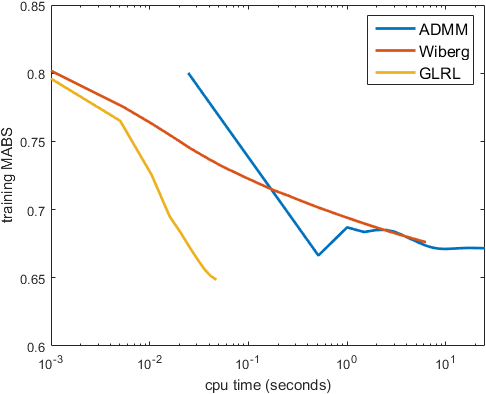
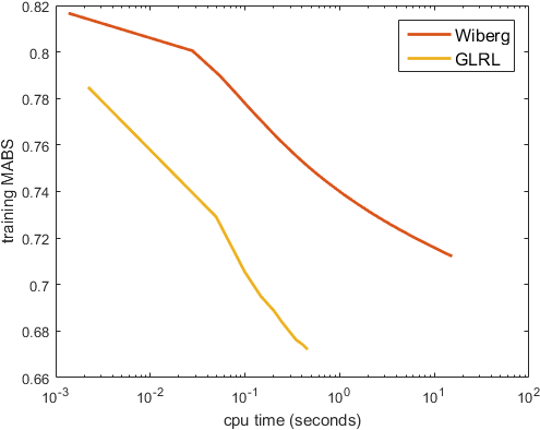
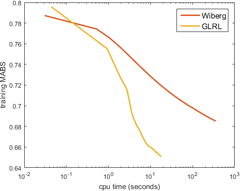
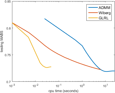
(a) 100K.

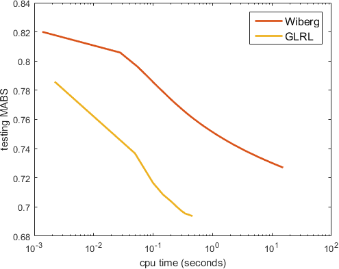
(b) 1M.

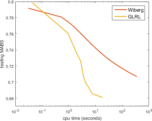
(c) 10M.

Figure 2: Training (top) and testing (bottom) MABS vs CPU time (seconds) on the MovieLens data sets.

5.2 Robust Matrix Factorization

Instead of using the square loss, robust matrix factorization uses the $\ell_{1}$ loss to reduce sensitivities to outliers Candès et al. (2011). This can be formulated as the optimization problem Lin et al. (2010):

$$\min_{X}\sum_{(i,j)\in\Omega}\left|X_{ij}-O_{ij}\right|\;\text{s.t.}\;\text{rank}(X)\leq r.$$

Note that the objective is only general convex, and its subgradient is bounded ($\leq\|\Omega\|_{F}$). Since there is no smooth component in the objective, AIS-Impute and AltMin cannot be used. Instead, we compare GLRL in Algorithm 3 (with $\nu=0.99$ and $c_{2}=0.05$) with the following:

1. Alternating direction method of multipliers (ADMM) Lin et al. (2010): The rank constraint is replaced by the nuclear norm regularizer, and ADMM Boyd et al. (2011) is then used to solve the equivalent problem: $\min_{X,Y}\sum_{(i,j)\in\Omega}|X_{ij}-O_{ij}|+\lambda\|Y\|_{*}\;\text{s.t.}\;Y=X$.

2. The Wiberg algorithm Eriksson and van den Hengel (2012): It factorizes $X$ into $UV^{\top}$ and optimizes them by linear programming. Here, we use the linear programming solver in Matlab.

Experiments are performed on the MovieLens data sets (Table 3), which have been commonly used for evaluating recommender systems Wang et al. (2014). They contain ratings $\{1,2,\dots,5\}$ assigned by various users on movies. The setup is the same as in Wang et al. (2014). $50\%$ of the ratings are randomly sampled for training while the rest for testing. The ranks used for the 100K, 1M, 10M data sets are 10, 10, and 20, respectively. For performance evaluation, we use the mean absolute error on the unobserved entries $\Omega^{\perp}$:

$$\text{MABS}=\frac{1}{||\Omega^{\perp}||_{1}}\sum_{(i,j)\in\Omega^{\perp}}|\hat{X}_{ij}-O_{ij}|,$$

where $\hat{X}$ is the predicted matrix Eriksson and van den Hengel (2012). Experiments are repeated five times with random training/testing splits.

Table 3: MovieLens data sets used in the experiments.

	#users	#movies	#ratings
100K	943	1,682	$10^{5}$
1M	6,040	3,449	$10^{6}$
10M	69,878	10,677	$10^{7}$

Results are shown in Table 4. As can be seen, ADMM performs slightly better on the 100K data set, and GLRL is more accurate than Wiberg. However, ADMM is computationally expensive as SVD is required in each iteration. Thus, it cannot be run on the larger 1M and 10M data sets. Figure 2 shows the convergence of MABS with CPU time. As can be seen, GLRL is the fastest, which is then followed by Wiberg, and ADMM is the slowest.

Table 4: Testing MABS on the MovieLens data sets. The best results (according to the pairwise t-test with 95% confidence) are highlighted. ADMM cannot converge in $1000$ seconds on the 1M and 10M data sets, and thus is not shown.

	100K	1M	10M
ADMM	0.717$\pm$0.004	—	—
Wiberg	0.726$\pm$0.001	0.728$\pm$0.006	0.715$\pm$0.005
GLRL	0.724$\pm$0.004	0.694$\pm$0.001	0.683$\pm$0.001

6 Conclusion

In this paper, we propose an efficient greedy algorithm for the learning of generalized low-rank models. Our algorithm is based on the state-of-art R1MP algorithm, but allows the optimization objective to be smooth or nonsmooth, general convex or strongly convex. Convergence analysis shows that the proposed algorithm has fast convergence rates, and is compatible with those obtained on other (convex) smooth/nonsmooth optimization problems. Specifically, on smooth problems, it converges with a rate of $O(1/T)$ on general convex problems and a linear rate on strongly convex problems. On nonsmooth problems, it converges with a rate of $O(1/\sqrt{T})$ on general convex problems and $O(\log(T)/T)$ rate on strongly convex problems. Experimental results on link prediction and robust matrix factorization show that the proposed algorithm achieves comparable or better prediction performance as the state-of-the-art, but is much faster.

Proposition 1

Proof.

At the $t$th iteration, we have $X_{t-1}=\sum_{i=1}^{t-1}\theta_{i}u_{i}v_{i}^{\top}$. Construct $\bar{\theta}=\left[\bar{\theta}_{i}\right]\in\mathbb{R}^{t}$ as

$$\bar{\theta}_{i}=\begin{cases}\theta_{i}&i<t\\ -s_{t}/L&i=t\end{cases},$$

and let $\bar{X}_{t}=\sum_{i=1}^{t}\bar{\theta}_{i}u_{i}v_{i}^{\top}$. Thus, $\bar{X}_{t}-X_{t-1}=-s_{t}u_{t}v_{t}^{\top}/L$. As $f$ is $L$-Lipschitz smooth,

$$f(\bar{X}_{t}) \leq f(X_{t-1})+\langle\bar{X}_{t}-X_{t-1},\nabla f(X_{t-1})\rangle$$ (12)

$$+\frac{L}{2}\|\bar{X}_{t}-X_{t-1}\|_{F}^{2}.$$

Note that $u_{t}^{\top}\nabla f(X_{t-1})v_{t}=s_{t}$. Together with (12), we have

$$f(\bar{X}_{t})\leq f(X_{t-1})-\frac{1}{2L}\langle\nabla f(X_{t-1}),u_{t}v_{t}^{\top}\rangle^{2}.$$ (13)

For the second term on the RHS of (13),

$$\left\langle\nabla f(X_{t-1}),u_{t}v_{t}^{\top}\right\rangle =\gamma_{t-1}\|\nabla f(X_{t-1})\|_{F}\|u_{t}v_{t}^{\top}\|_{F}$$

$$=\gamma_{t-1}\|\nabla f(X_{t-1})\|_{F},$$

where $\gamma_{t-1}=\frac{\left\langle\nabla f(X_{t-1}),u_{t}v_{t}^{\top}\right\rangle}{\|\nabla f(X_{t-1})\|_{F}}$. Note that $s_{t}$ is the largest singular value of $\nabla f(X_{t-1})$. Thus, $s_{t}\geq\|\nabla f(X_{t-1})\|_{F}/\sqrt{m}$, and

$$\gamma_{t-1}=\frac{s_{t}}{\|\nabla f(X_{t-1})\|_{F}}\in[1/\sqrt{m},1]$$

Then (13) becomes

$$f(\bar{X}_{t})\leq f(X_{t-1})-\frac{\gamma_{t-1}^{2}}{2L}\|\nabla f(X_{t-1})\|_{F}^{2}.$$

In Algorithm 2, $X_{t}$ is obtained by minimizing $\theta_{t}$ over (6) or (7). Once we warm start $\theta$ using $\bar{\theta}$, we can ensure that $f(X_{t})\leq f(\bar{X}_{t})$, and thus the Proposition holds. ∎

Theorem 2

Lemma 7.

If $f$ is $\mu$-strongly convex, $f(Y)\geq f(X)-\frac{1}{2\mu}\|\nabla f(X)\|_{F}^{2}$ for any $X,Y$.

Proof.

Since $f$ is $\mu$-strongly convex,

$$f(Y) \geq f(X)+\left\langle\nabla f(X),Y-X\right\rangle+\frac{\mu}{2}\|Y-X\|_{F}^{2}$$

$$\geq\min_{\bar{Y}}f(X)+\left\langle\nabla f(X),\bar{Y}-X\right\rangle+\frac{\mu}{2}\|\bar{Y}-X\|_{F}^{2}.$$

The minimum is achieved at $\bar{Y}=X-\frac{1}{\mu}\nabla f(X)$, and $f(\bar{Y})=f(X)-\frac{1}{2\mu}\|\nabla f(X)\|_{F}^{2}$. ∎

Proof.

On optimal $\nabla f(X_{*})=0$, using Lemma 7:

$$\|\nabla f(X_{t-1})-\nabla f(X_{*})\|_{F}^{2}\geq 2\mu\left[f(X_{t-1})-f(X_{*})\right].$$ (14)

Combine it with Proposition 1, then

$$f(X_{t})-f(X_{*})$$

$$\leq\left[f(X_{t-1})-f(X_{*})\right]-\frac{(\gamma_{t-1})^{2}}{2L}\|\nabla f(X_{t-1})\|_{F}^{2},$$

$$\leq(1-\frac{\mu(\gamma_{t-1})^{2}}{L})\left[f(X_{t-1})-f(X_{*})\right],$$

$$\leq(1-\frac{\mu d_{1}^{2}}{L})\left[f(X_{t-1})-f(X_{*})\right]$$

Induct from $t=1$ to $t=T$, we then have the Theorem. ∎

Theorem 3

First, we show that $\{\|X_{t}-X_{*}\|_{F}\}$ is upper-bounded.

Proposition 8.

For $\{X_{t}\}$ generated by Algorithm 2, $\max_{t=1}^{T}\|X_{t}-X_{*}\|_{F}\leq d_{2}$ for some $d_{2}$.

Proof.

Let $A_{t}=f(X_{t})-f(X_{*})$, from Proposition 1

$$A_{t-1}-A_{t}\geq\frac{d_{1}^{2}}{2L}\|\nabla f(X_{t-1})\|_{F}^{2}.$$ (15)

Summing (15) from $t=1$ to $T$, then

$$\sum_{t=1}^{T}\frac{d_{1}^{2}}{2L}\|\nabla f(X_{t-1})\|_{F}^{2} \leq\sum_{t=1}^{T}\left(A_{t-1}-A_{t}\right)$$

$$=A_{0}-A_{T}\leq A_{0}$$

Since $f(X)$ is lower bounded, thus on $T=+\infty$, we must have $\nabla f(X_{t-1})=0$, i.e. $X_{t}$ is a convergent sequence to $X_{*}$ and will not diverse. As a result, there must exist a constant $d_{2}$ such that $\|X_{t}-X_{*}\|_{F}\leq d_{2}$. ∎

Now, we start to prove Theorem 3.

Proof.

From convexity, and since $f(X_{*})$ is the minimum, therefore, we have

$$\left\langle X_{t-1}-X_{*},\nabla f(X_{t-1})\right\rangle\geq f(X_{t-1})-f(X_{*})\geq 0.$$

Next, since $\nabla f(X_{*})=0$ and use Cauchy inequality $\left\langle X,Y\right\rangle\leq\|X\|_{F}\|Y\|_{F}$, then

$$f(X_{t-1})-f(X_{*})$$

$$\quad\leq\left\langle X_{t-1}-X_{*},\nabla f(X_{t-1})-\nabla f(X_{*})\right\rangle$$

$$\quad\leq\|X_{t-1}-X_{*}\|_{F}\|\nabla f(X_{t-1})-\nabla f(X_{*})\|_{F}$$ (16)

Then, from Proposition 8, there exist a $d_{2}$ such that $\|X_{t-1}-X_{*}\|_{F}\leq d_{2}$, combining it with (16), we have:

$$\|\nabla f(X_{t-1})-\nabla f(X_{*})\|_{F}\geq\frac{1}{d_{2}}\left[f(X_{t-1})-f(X_{*})\right]$$

Combine above inequality with Proposition 1,

$$A_{t} \leq A_{t-1}-\frac{d_{1}^{2}}{2L}\|\nabla f(X_{t-1})-\nabla f(X_{*})\|_{F}^{2}$$

$$\leq A_{t-1}-\frac{d_{1}^{2}}{2Ld_{2}^{2}}A_{t-1}^{2}.$$

Therefore, by Lemma B.2 of Shalev-Shwartz et al. (2010), the above sequence converges to $0$ of rate

$$f(X_{T})-f(X_{*})\leq\frac{2Ld_{2}^{2}A_{0}}{d_{1}^{2}TA_{0}+2Ld_{2}^{2}}.$$

which proves the Theorem. ∎

Theorem 4

Proof.

When restrict to $\Omega$ in (2):

$$\ell(X)\leq\;\ell(Y)+\left\langle P_{\Omega}(X-Y),\nabla\ell(Y)\right\rangle+\frac{1}{2}\|P_{\Omega}(X-Y)\|_{F}^{2}.$$

On optimal $\nabla\ell(X_{*})=0$, using above inequality, then

$$\ell(X_{t-1})\leq\ell(X_{*})+\frac{1}{2}\|\nabla\ell(X_{t-1})-\nabla\ell(X_{*})\|_{F}^{2}$$

As a result, we get

$$\|\nabla\ell(X_{t-1})-\nabla\ell(X_{*})\|_{F}^{2}\geq 2\left[\ell(X_{t-1})-\ell(X_{*})\right]$$ (17)

Since $\ell$ is $1$-Lipschitz smooth and $\nabla\ell(X_{*})=0$, together with Proposition 1 and (17), then

$$\ell(X_{t})-\ell(X_{*}) \leq\left[\ell(X_{t-1})-\ell(X_{*})\right]-\frac{d_{1}^{2}}{2}\|\nabla\ell(X_{t-1})\|_{F}^{2},$$

$$\leq\left(1-d_{1}^{2}\right)\left[\ell(X_{t-1})-\ell(X_{*})\right].$$

Induct from $t=1$ to $t=T$, we then have

$$\ell(X_{T})-\ell(X_{*})\leq\left(1-d_{1}^{2}\right)^{T}\left[\ell(X_{0})-\ell(X_{*})\right].$$

Thus, we get the Theorem, and linear rate exists. ∎

Theorem 5

Proof follows Theorem 5 at Grubb and Bagnell (2011).

Proof.

$$\|X_{t}-X_{*}\|_{F}^{2}$$

$$= \|X_{t-1}-X_{*}-\eta_{t}h_{t}\|_{F}^{2}$$

$$= \|X_{t-1}-X_{*}\|_{F}^{2}+\eta_{t}^{2}\|h_{t}\|_{F}^{2}-2\eta_{t}\left\langle h_{t},X_{t-1}-X_{*}\right\rangle$$

$$= \|X_{t-1}-X_{*}\|_{F}^{2}-2\eta_{t}\left\langle g_{t},X_{t-1}-X_{*}\right\rangle$$

$$-2\eta_{t}\left\langle h_{t}-g_{t},X_{t-1}-X_{*}\right\rangle+\eta_{t}^{2}\|h_{t}\|_{F}^{2}.$$

Rearranging items, we have:

$$\left\langle g_{t},X_{t-1}-X_{*}\right\rangle$$ (18)

$$= \frac{1}{2\eta_{t}}\|X_{t-1}-X_{*}\|_{F}^{2}-\frac{1}{2\eta_{t}}\|X_{t}-X_{*}\|_{F}^{2}$$

$$+\frac{\eta_{t}}{2}\|h_{t}\|_{F}^{2}-\left\langle h_{t}-g_{t},X_{t-1}-X_{*}\right\rangle.$$

As $f$ is $\mu$-strongly convex,

$$f(X_{*}) \geq f(X_{t-1})+\left\langle g_{t},X_{*}-X_{t-1}\right\rangle$$ (19)

$$+\frac{\mu}{2}\|X_{t-1}-X_{*}\|_{F}^{2}.$$

Sum (19) from $t=1$ to $T$, and using (18)

$$\sum_{t=1}^{T}f(X_{*})$$ (20)

$$\geq \sum_{t=1}^{T}f(X_{t-1})+\left\langle g_{t},X_{*}-X_{t-1}\right\rangle+\frac{\mu}{2}\|X_{t-1}-X_{*}\|_{F}^{2}$$

$$\geq \sum_{t=1}^{T}\left\{f(X_{t-1})-\frac{\eta_{t}}{2}\|h_{t}\|_{F}^{2}-\left\langle X_{*}-X_{t-1},h_{t}-g_{t}\right\rangle\right\}$$

$$+\frac{1}{2}\sum_{t=1}^{T-1}(\frac{1}{\eta_{t}}-\frac{1}{\eta_{t+1}}+\mu)\|X_{t}-X_{*}\|_{F}^{2}$$

$$+\frac{1}{2}(\mu-\frac{1}{\eta_{1}})\|X_{0}-X_{*}\|_{F}^{2}+\frac{1}{2\eta_{T}}\|X_{T}-X_{*}\|_{F}$$

$$\geq \sum_{t=1}^{T}\left\{f(X_{t-1})-\frac{\eta_{t}}{2}\|h_{t}\|_{F}^{2}-\left\langle X_{*}-X_{t-1},h_{t}-g_{t}\right\rangle\right\}$$

$$+\frac{1}{2}\sum_{t=0}^{T-1}(\frac{1}{\eta_{t}}-\frac{1}{\eta_{t+1}}+\mu)\|X_{t}-X_{*}\|_{F}^{2}$$

$$-\frac{1}{2\eta_{0}}\|X_{0}-X_{*}\|_{F}^{2}$$

Recall, the step size is $\eta_{t}=c_{1}/t$, then (20) becomes

$$\sum_{t=1}^{T}f(X_{*})$$ (21)

$$\geq \sum_{t=1}^{T}f(X_{t-1})-\frac{c_{1}}{2}\sum_{t=1}^{T}\frac{1}{t}\|h_{t}\|_{F}^{2}$$

$$+\frac{1}{2}\left(\mu-\frac{1}{c_{1}}\right)\sum_{t=1}^{T}\|X_{t-1}-X_{*}\|_{F}^{2}-\frac{1}{2c_{1}}\|X_{0}-X_{*}\|_{F}^{2}$$

$$-\sum_{t=1}^{T}\left\langle X_{*}-X_{t-1},h_{t}-g_{t}\right\rangle$$

where $\eta_{0}$ is can be picked up as $c_{1}$. For the second term in (21), it is simply bounded as

$$\frac{c_{1}}{2}\sum_{t=1}^{T}\frac{\|h_{t}\|_{F}^{2}}{t} \leq\frac{c_{1}}{2}\sum_{t=1}^{T}\frac{b_{1}^{2}}{t}$$

$$\leq\frac{c_{1}b_{1}^{2}}{2}\left(1+\log(T)\right).$$ (22)

Let $\hat{c}=\frac{1}{2}\left(\mu-\frac{1}{c_{1}}\right)$, since $c_{1}\geq\frac{1}{\mu}$, thus $\hat{c}\geq 0$. For last term in (21), we use $\|A\|_{F}^{2}+2\left\langle A,B\right\rangle\geq-\|B\|_{F}^{2}$, let $A=X_{t}-X_{*}$ and $B=\frac{1}{2\hat{c}}(h_{t}-g_{t})$, then

$$\hat{c}\sum_{t=1}^{T}\left(\|X_{t}-X_{*}\|_{F}^{2}+\frac{1}{\hat{c}}\left\langle X_{t}-X_{*},h_{t}-g_{t}\right\rangle\right)$$

$$\geq-\hat{c}\sum_{t=1}^{T}\|\frac{1}{2\hat{c}}(h_{t}-g_{t})\|_{F}^{2}=-\frac{1}{4\hat{c}}\sum_{t=1}^{T}\|h_{t}-g_{t}\|_{F}^{2}$$ (23)

By definition of $h_{t}$ and assumption $\max_{t=1}^{T}\|g_{t}\|_{F}\leq b_{1}$, for the first iteration ($t=1$)

$$\|h_{1}-g_{1}\|_{F}^{2} =\|s_{1}(u_{1}v_{1}^{\top})+g_{1}\|_{F}^{2}$$

$$=(s_{1})^{2}+2s_{1}\left\langle u_{1}v_{1}^{\top},g_{1}\right\rangle+\|g_{1}\|_{F}^{2}$$

$$\leq 4\|g_{1}\|_{F}^{2}=4b_{1}^{2}.$$

In Algorithm 3, we ensure

$$\|h_{t}-g_{t}\|_{F}^{2}\leq\nu\|h_{t-1}-g_{t-1}\|_{F}^{2}$$

thus (23) becomes:

$$\sum_{t=1}^{T}\|h_{t}-g_{t}\|_{F}^{2} \leq 4\sum_{t=1}^{T}\nu^{t-1}b_{1}^{2}$$

$$\leq 4\sum_{t=1}^{+\infty}\nu^{t-1}b_{1}^{2}=\frac{4b_{1}^{2}}{1-\nu}.$$ (24)

Now, using (22) and (24), we can bound (21) as

$$\sum_{t=1}^{T}f(X_{*}) \geq\sum_{t=1}^{T}f(X_{t-1})-\frac{c_{1}b_{1}^{2}}{2}\left(1+\log(T)\right)$$

$$-\frac{1}{2c_{1}}\|X_{0}-X_{*}\|_{F}^{2}-\frac{b_{1}^{2}}{(1-\nu)\hat{c}}.$$

Thus, we can get convergence rate as

$$\min_{t=0,\cdots,T-1}\left[f(X_{t})-f(X_{*})\right]T$$

$$\leq\sum_{t=1}^{T}\left[f(X_{t-1})-f(X_{*})\right]$$

$$\leq\left(1+\log(T)\right)\frac{c_{1}b_{1}^{2}}{2}+\frac{1}{2c_{1}}\|X_{0}-X_{*}\|_{F}^{2}+\frac{b_{1}^{2}}{(1-\nu)\hat{c}}.$$

Finally, note that

$$\min_{t=0,\cdots,T}f(X_{t})-f(X_{*})\leq\min_{t=0,\cdots,T-1}f(X_{t})-f(X_{*})$$ (25)

Let $b_{2}=\frac{1}{2c_{1}}\|X_{0}-X_{*}\|_{F}^{2}+\frac{b_{1}^{2}}{(1-\nu)\hat{c}}$, we get the theorem. ∎

Theorem 6

Proof follows Theorem 6 at Grubb and Bagnell (2011). First, we introduce below Proposition

Proposition 9 (Beardon (1996)).

Given $k>0$, the approximation of sum over natural numbers is:

$$\sum_{t=1}^{T}t^{k}\leq\frac{(T+0.5)^{k+1}}{k+1}.$$

Now, we start to prove Theorem 6.

Proof.

For weak convex convexity (obtained from (20) with $\mu=0$), we have

$$\sum_{t=1}^{T}f(X_{*}) \geq\sum_{t=1}^{T}f(X_{t-1})-\frac{1}{2\eta_{0}}\|X_{0}-X_{*}\|_{F}^{2}$$ (26)

$$\quad+\frac{1}{2}\sum_{t=0}^{T-1}\left(\frac{1}{\eta_{t}}-\frac{1}{\eta_{t+1}}\right)\|X_{t}-X_{*}\|_{F}^{2}$$

$$\quad-\sum_{t=1}^{T}\frac{\eta_{t}}{2}\|h_{t}\|_{F}^{2}-\sum_{t=1}^{T}\left\langle X_{*}-X_{t-1},h_{t}-g_{t}\right\rangle$$

where $\eta_{0}$ is picked up at $c_{2}$. The step size is $\eta_{t}=c_{2}/\sqrt{t}$, use it back into (26), we get

$$\sum_{t=1}^{T}f(X_{*})$$

$$\geq \sum_{t=1}^{T}f(X_{t-1})-\frac{1}{2c_{2}}\|X_{0}-X_{*}\|_{F}^{2}$$

$$+\frac{c_{2}}{2}\sum_{t=1}^{T-1}\left(\frac{1}{\sqrt{t}}-\frac{1}{\sqrt{t+1}}\right)\|X_{t}-X_{*}\|_{F}^{2}$$

$$-\sum_{t=1}^{T}\frac{c_{2}}{2\sqrt{t}}\|h_{t}\|_{F}^{2}-\sum_{t=1}^{T}\left\langle X_{*}-X_{t-1},h_{t}-g_{t}\right\rangle$$

$$\geq \sum_{t=1}^{T}f(X_{t-1})-\frac{c_{2}}{2}\sum_{t=1}^{T}\frac{1}{\sqrt{t}}\|X_{t}-X_{*}\|_{F}^{2}$$

$$-\sum_{t=1}^{T}\frac{c_{2}}{2\sqrt{t}}\|h_{t}\|_{F}^{2}-\sum_{t=1}^{T}\left\langle X_{*}-X_{t-1},h_{t}-g_{t}\right\rangle$$

$$\geq \sum_{t=1}^{T}f(X_{t-1})-\frac{c_{2}}{2}\sum_{t=1}^{T}\frac{1}{\sqrt{t}}\|X_{t}-X_{*}\|_{F}^{2}$$

$$-\frac{c_{2}}{2}\sum_{t=1}^{T}\frac{1}{\sqrt{t}}\|h_{t}\|_{F}^{2}-\sum_{t=1}^{T}\|X_{*}-X_{t-1}\|_{F}\|h_{t}-g_{t}\|_{F}$$

where the second inequality comes from the fact $1/\sqrt{t}-1/\sqrt{t+1}\geq-1/\sqrt{t}$. For the last term in (Proof.), since $\|X_{*}-X_{t-1}\|_{F}\leq b_{3}$ and $\|h_{1}-g_{1}\|_{F}\leq 2b_{1}$, it can be bounded as

$$\sum_{t=1}^{T} \|X_{*}-X_{t-1}\|_{F}\|h_{t}-g_{t}\|_{F}$$

$$\leq b_{3}\sum_{t=1}^{T}\|h_{t}-g_{t}\|_{F}\leq b_{3}\sum_{t=1}^{T}(\sqrt{\nu})^{t-1}\|h_{1}-g_{1}\|_{F}$$

$$\leq 2b_{1}b_{3}\sum_{t=1}^{+\infty}(\sqrt{\nu})^{t-1}=\frac{2b_{1}b_{3}}{1-\sqrt{\nu}}$$ (28)

Then, note that $\|h_{t}\|_{F}\leq\|g_{t}\|_{F}\leq b_{1}$, use (Proof.) and (28)

$$\sum_{t=1}^{T}f(X_{*}) \geq\sum_{t=1}^{T}f(X_{t-1})-\frac{c_{2}(b_{3}^{2}+b_{1}^{2})}{2}\sum_{t=1}^{T}\frac{1}{\sqrt{t}}-\frac{2b_{1}b_{3}}{1-\sqrt{\nu}}$$

Rearrange items in above inequality, from Proposition 9:

$$\min_{t=0,\cdots,T-1} \left[f(X_{t})-f(X_{*})\right]$$

$$\leq\frac{1}{T}\sum_{t=1}^{T}\left[f(X_{t-1})-f(X_{*})\right]$$

$$\leq\frac{c_{2}(b_{1}^{2}+b_{3}^{2})}{2T}\sum_{t=1}^{T}\frac{1}{\sqrt{t}}-\frac{2b_{1}b_{3}}{(1-\sqrt{\nu})T}$$

$$\leq\frac{c_{2}(b_{1}^{2}+b_{3}^{2})}{2\sqrt{T}}-\frac{2b_{1}b_{3}}{(1-\sqrt{\nu})T}$$

Finally, using (25) we get the Theorem. ∎

References

- Argyriou et al. [2006] A. Argyriou, T. Evgeniou, and M. Pontil. Multi-task feature learning. In Advances in Neural Information Processing Systems, pages 41–48, 2006.
- Beardon [1996] A.F. Beardon. Sums of powers of integers. The American Mathematical Monthly, 103(3):201–213, 1996.
- Beck and Teboulle [2009] A. Beck and M. Teboulle. A fast iterative shrinkage-thresholding algorithm for linear inverse problems. SIAM Journal on Imaging Sciences, 2(1):183–202, 2009.
- Boyd et al. [2011] S. Boyd, N. Parikh, E. Chu, B. Peleato, and J. Eckstein. Distributed optimization and statistical learning via the alternating direction method of multipliers. Foundations and Trends in Machine Learning, 3(1):1–122, 2011.
- Candès and Recht [2009] E.J. Candès and B. Recht. Exact matrix completion via convex optimization. Foundations of Computational Mathematics, 9(6):717–772, 2009.
- Candès et al. [2011] E.J. Candès, X. Li, Y. Ma, and J. Wright. Robust principal component analysis? Journal of the ACM, 58(3):11:1–11:37, 2011.
- Chiang et al. [2014] K. Chiang, C. Hsieh, N. Natarajan, I.S. Dhillon, and A. Tewari. Prediction and clustering in signed networks: A local to global perspective. Journal of Machine Learning Research, 15(1):1177–1213, 2014.
- Eriksson and van den Hengel [2012] A. Eriksson and A. van den Hengel. Efficient computation of robust weighted low-rank matrix approximations using the norm. IEEE Transactions on Pattern Analysis and Machine Intelligence, 34(9):1681–1690, 2012.
- Grubb and Bagnell [2011] A. Grubb and D. Bagnell. Generalized boosting algorithms for convex optimization. In Proceedings of the 28th International Conference on Machine Learning (ICML-11), pages 1209–1216, 2011.
- Halko et al. [2011] N. Halko, P. Martinsson, and J.A. Tropp. Finding structure with randomness: Probabilistic algorithms for constructing approximate matrix decompositions. SIAM Review, 53(2):217–288, 2011.
- Hsieh and Olsen [2014] C. Hsieh and P. Olsen. Nuclear norm minimization via active subspace selection. In Proceedings of the 31st International Conference on Machine Learning, pages 575–583, 2014.
- Jaggi [2013] M. Jaggi. Revisiting Frank-Wolfe: Projection-free sparse convex optimization. In Proceedings of the 30th International Conference on Machine Learning, pages 427–435, 2013.
- Koenker [2005] R. Koenker. Quantile Regresssion. Cambridge University Press, 2005.
- Lin et al. [2010] Z. Lin, M. Chen, and Y. Ma. The augmented Lagrange multiplier method for exact recovery of corrupted low-rank matrices. Technical report arXiv:1009.5055, 2010.
- Mazumder et al. [2010] R. Mazumder, T. Hastie, and R. Tibshirani. Spectral regularization algorithms for learning large incomplete matrices. Journal of Machine Learning Research, 11:2287–2322, 2010.
- Nocedal and Wright [2006] J. Nocedal and S.J. Wright. Numerical Optimization. Springer, 2006.
- Pati et al. [1993] Y.C. Pati, R. Rezaiifar, and P.S. Krishnaprasad. Orthogonal matching pursuit: Recursive function approximation with applications to wavelet decomposition. In Proceedings of the 27th Asilomar Conference on Signals, Systems and Computers, pages 40–44, 1993.
- Recht et al. [2010] B. Recht, M. Fazel, and P. Parrilo. Guaranteed minimum-rank solutions of linear matrix equations via nuclear norm minimization. SIAM Review, 52(3):471–501, 2010.
- Shalev-Shwartz et al. [2010] S. Shalev-Shwartz, N. Srebro, and T. Zhang. Trading accuracy for sparsity in optimization problems with sparsity constraints. SIAM Journal on Optimization, 20(6):2807–2832, 2010.
- Shalev-shwartz et al. [2011a] S. Shalev-shwartz, A. Gonen, and O. Shamir. Large-scale convex minimization with a low-rank constraint. In Proceedings of the 28th International Conference on Machine Learning, pages 329–336, 2011.
- Shalev-Shwartz et al. [2011b] S. Shalev-Shwartz, Y. Singer, N. Srebro, and A. Cotter. Pegasos: Primal estimated sub-gradient solver for SVM. Mathematical Programming, 127(1):3–30, 2011.
- Srebro et al. [2004] N. Srebro, J. Rennie, and T.S. Jaakkola. Maximum-margin matrix factorization. In Advances in Neural Information Processing Systems, pages 1329–1336, 2004.
- Tai and Lin [2012] F. Tai and H. Lin. Multilabel classification with principal label space transformation. Neural Computation, 24(9):2508–2542, 2012.
- Udell et al. [2015] M. Udell, C. Horn, R. Zadeh, and S. Boyd. Generalized low rank models. Technical Report arXiv:1410.0342, 2015.
- Wang et al. [2014] Z. Wang, M. Lai, Z. Lu, W. Fan, H. Davulcu, and J. Ye. Rank-one matrix pursuit for matrix completion. In Proceedings of the 31st International Conference on Machine Learning, pages 91–99, 2014.
- Wen et al. [2012] Z. Wen, W. Yin, and Y. Zhang. Solving a low-rank factorization model for matrix completion by a nonlinear successive over-relaxation algorithm. Mathematical Programming Computation, 4(4):333–361, 2012.
- Yao and Kwok [2015] Q. Yao and J.T. Kwok. Accelerated inexact soft-impute for fast large-scale matrix completion. In Proceedings of the 24th International Joint Conference on Artificial Intelligence, pages 4002–4008, 2015.
- Yao et al. [2015] Q. Yao, J.T. Kwok, and W. Zhong. Fast low-rank matrix learning with nonconvex regularization. In Proceedings of the International Conference on Data Mining, pages 539–548, 2015.
- Yu et al. [2014] H. Yu, P. Jain, P. Kar, and I.S. Dhillon. Large-scale multi-label learning with missing labels. In Proceedings of the 31st International Conference on Machine Learning, pages 593–601, 2014.
- Zhang et al. [2012] X. Zhang, D. Schuurmans, and Y. Yu. Accelerated training for matrix-norm regularization: A boosting approach. In Advances in Neural Information Processing Systems, pages 2906–2914, 2012.