Factorization of the dijet cross section in hadron-hadron collisions

Abstract

The factorization theorem for the dijet cross section is presented in hadron-hadron collisions with a cone-type jet algorithm. We also apply the beam veto to the beam jets consisting of the initial radiation. The soft-collinear effective theory is employed to see the factorization structure transparently when there are four distinct lightcone directions involved. There are various types of divergences such as the ultraviolet and infrared divergences. And when the phase space is divided to probe the collinear and the soft parts, there appears an additional divergence called rapidity divergence. These divergences are sorted out and we will show that all the infrared and rapidity divergences cancel, and only the ultraviolet divergence remains. It is a vital step to justify the factorization. Among many partonic processes, we take $q\overline{q}\rightarrow gg$ as a specific example to consider the dijet cross section. The hard and the soft functions have nontrivial color structure, while the jet and the beam functions are diagonal in operator basis. The dependence of the soft anomalous dimension on the jet algorithm and the beam veto is diagonal in operator space, and is cancelled by that of the jet and beam functions. We also compute the anomalous dimensions of the factorized components, and resum the large logarithms to next-to-leading logarithmic accuracy by solving the renormalization group equation.

I Introduction

The study of jet physics in high energy scattering has reached a sophisticated level. Many of the factorization theorems for inclusive scattering processes have been established both in QCD and in soft-collinear effective theory (SCET) Bauer et al. (2000, 2001, 2002). More differential quantities such as the transverse momentum dependence of the final-state particles or jets Stewart et al. (2014), and the jet substructures Dasgupta et al. (2013) have been studied. When we probe more differential quantities, the factorization theorems should be first proved in order that each factorized part can be computed in perturbation theory offering predictive power.

In general, the factorization theorem states that the expression for physical observables is written as the product or the convolution of the hard, the collinear and the soft parts. In proving the factorization theorem, it is important to verify that each factorized part is infrared (IR) finite. Otherwise the dependence of the renormalization scale does not solely come from the ultraviolet (UV) divergence, which invalidates the scaling behavior of the factorized parts. If some components are not IR finite in the factorized form, the factorized parts should be refactorized such that the redefined or rearranged quantities are IR finite. If the IR divergence still remains even after the rearrangement, the quantity at hand is not physical.

A fully inclusive quantity is IR finite to all orders due to the Kinoshita-Lee-Nauenberg theorem Kinoshita (1962); Lee and Nauenberg (1964) since the IR divergence from the virtual contribution is cancelled by that of the real contribution. It should hold true also for exclusive physical quantities such as the dijet cross section, even though the phase space for the real gluon emission is constrained by the jet algorithm and the beam veto. However, large logarithms appear due to the slight mismatch of the phase spaces for the virtual and real contributions.

The verification that each factorized part is IR finite in the dijet cross section from $e^{+}e^{-}$ annihilation with various jet algorithms has been performed in Refs.Chay et al. (2015a, b). On the other hand, here we take the dijet cross section in hadron-hadron collision with a cone-type jet algorithm Salam (2010) to establish the factorization theorem by carefully dissecting the phase space and performing the corresponding computation. This process is more complicated due to the complex color structure and the existence of the beam jets, thus more illuminating to show how to disentangle the interwoven structure of the dependence of the cross section on the jet algorithms and the beam veto.

We employ SCET to present the factorization theorem for the dijet cross section because it is the appropriate effective theory to describe this process. The advantage of SCET is to establish the decoupling between the collinear and the soft modes at the operator level, thus the factorization procedure manifest. However, as far as the structure of the divergence is concerned, there is another type of divergence, called the rapidity divergence Chiu et al. (2012a, b) in SCET. It appears because we dissect the phase space into the collinear and the soft regions, and the soft region with small rapidity does not recognize the collinear region with large rapidity. In the full theory, there is no such divergence because there is no kinematic constraint. It is a good consistency check for the effective theory to see physical observables are free of the rapidity divergence. We show that the factorized parts do not have the rapidity divergence, though the individual contribution may possess one. If a physical observable is more differential, there may exist rapidity divergence in the collinear and soft parts separately, though they cancel in the total contribution. This rapidity divergence contributes to the additional renormalization group (RG) evolution. However, it is not our topic in this paper because there is no rapidity divergence in each factorized part in the inclusive jet cross section.

The dijet cross section in hadron-hadron collision is shown to be factorized into the hard, collinear and soft parts, which is schematically written as

$$\sigma_{J}\sim\mathrm{tr}(\mathbf{H}\otimes\mathbf{S})\otimes B_{i/N_{1}}\otimes B_{j/N_{2}}\otimes\mathcal{J}_{3}\otimes\mathcal{J}_{4}.$$ (1)

A more rigorous expression will be derived in Sec. II. Here $\mathbf{H}$ is the hard function depending only on the hard scales, and $\mathbf{S}$ is the soft function which describes the soft radiations interspersed between the energetic particles. The hard and soft functions are matrices in color space because they arise from different color channels. The incoming partons emit particles in the initial radiation, and the off-shell partons participate in the hard scattering. These processes are described by the beam functions $B_{i/N}$, for the parton $i$ entering into the hard interaction from the hadron $N$ Stewart et al. (2010). And $\mathcal{J}_{i}$ are the integrated jet functions describing the outgoing collinear particles in the final state, prescribed by a jet algorithm.

The RG evolution of the functions in Eq. (1) resums a large set of logarithms. In providing factorization, there is a hierarchy of scales. The hard scale is characterized by $Q$, the collinear scale is $Q\lambda$, and the soft scale is $Q\lambda^{2}$, where $\lambda$ is a small parameter, appearing in SCET. Then at fixed order, there appears large logarithms with the ratios of these disparate scales, which may invalidate the perturbative series. Therefore these large logarithms should be resummed to all orders. In the dissected phase spaces, there appears only a singlet scale, and the resummation can be achieved by solving the RG equation for each factorized part. However, we note that there are other types of logarithms such as the logarithms of the small jet radius $R$ Alioli and Walsh (2014); Kelley et al. (2012) and nonglobal logarithms Dasgupta and Salam (2001); Banfi et al. (2002); Appleby and Salam (2003), which are big challenges. Here we take the jet radius $R$ to be not too small ($R\sim 0.7$), and do not perform the small $R$-resummation. And we will not consider the nonglobal logarithms either because we are mainly interested in the factorization structure with four lightlike directions in the process. Last but not least, we assume that the Glauber gluons, which are responsible for the interactions between the active partons and the spectator partons, do not violate factorization.

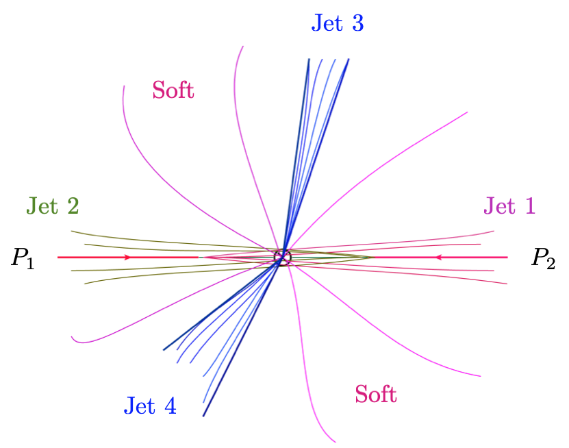
Figure 1: A schematic diagram for the dijet production in hadron-hadron scattering. From the hadrons with momenta $P_{1}$, and $P_{2}$, the partons, after emitting the initial-state radiation, with the momenta $p_{1}$ and $p_{2}$ undergo a hard scattering. Out of the hard scattering, the two jets with their momenta $p_{3}$ and $p_{4}$ are produced. The initial-state radiation produces beam jets. The soft momentum $p_{s}$ is either inside or outside the jets depending on the jet algorithm.

The configuration of the dijet production is sketched in Fig. 1. The incoming partons from the two hadrons with momenta $P_{1}$ and $P_{2}$ radiate the initial-state radiation, and finally have the momenta $p_{1}$ and $p_{2}$, and participate in the hard collision. The remnant produces the beam jets in the beam directions. The outgoing particles form collimated beams of collinear particles, called jets, and the jets are clustered depending on the jet algorithms being employed. Jet algorithms in $e^{+}e^{-}$ annihilation and in hadron-hadron scattering are different since the latter should preserve the boost invariance along the beam direction. However, the relations between the jet algorithms in the two cases are explained in Ref. Hornig et al. (2016), and we can employ the same cone-type jet algorithm with the rescaling of the jet radius accordingly. For central jets with the rapidity close to zero, the cone-type jet algorithms in both cases take the same form. On the other hand, the initial-state radiation also forms beam jets in the beam direction. The beam jets are constrained by the rapidity cutoff $y_{\mathrm{cut}}$ to be contained in the beam direction, which will be discussed in detail. It is called the beam veto.

In high-energy processes, there are hierarchies of scales involved at every stage of the scattering, and they should be entangled to sort out the effect of the strong interaction. This is the essence in the proof of the factorization, in which the hard, collinear and soft parts are factorized. Furthermore it is important to guarantee that each factorized part contains only the UV divergence without any IR divergence. Another aspect is the rapidity divergence. In SCET, the collinear and the soft regions are separated by the rapidities. The collinear modes have large rapidity, while the soft modes have small rapidity. In computing the soft radiative correction, it reaches the large rapidity region, which cannot be recognized by the soft mode, and this causes the rapidity divergence. If the collinear and the soft modes do not have the same offshellness, the rapidity divergence vanishes in each sector. However, when they have the same offshellness, the rapidity divergence may remain in each sector though their sum vanishes. This affects the RG evolution of the collinear and the soft parts.

Here we focus on the dijet cross section to illustrate how carefully the UV and IR divergences along with the rapidity divergence should be treated. We examine various radiative corrections to next-to-leading order (NLO) and show that each factorized part is indeed IR, and rapidity finite. This type of analysis should be applied to other various differential processes for the rigorous proof of the factorization theorems. Only after the remaining divergence is guaranteed to be of the UV origin, we can safely apply the RG equation to resum large logarithms. In this paper, we employ the pure dimensional regularization with the spacetime dimension $D=4-2\epsilon$ and the $\overline{\mathrm{MS}}$ scheme, in which we carefully distinguish the UV and the IR divergences in computing radiative corrections of the collinear and soft functions with a jet algorithm and a beam veto.

The dijet cross section is described by $2\to 2$ processes at the parton level. We can analyze all the processes for phenomenology, but we rather choose the specific process $q\overline{q}\to gg$ to show how to treat all the types of the divergences consistently. This process involves the computation of the gluon jet function with the jet algorithm Ellis et al. (2010), and the quark beam function with the beam veto. Note that the quark jet function with the jet algorithm was calculated in Ref. Chay et al. (2015a); Jouttenus (2010); Cheung et al. (2009). And the structure of the hard and soft functions is interesting and complicated enough to seek the consistency in the relations among the anomalous dimensions.

This paper is organized as follows: The factorization of the dijet cross section in hadron-hadron collision is presented in Sec. II. We take a specific example of the partonic process $q\overline{q}\rightarrow gg$ to express the individual factorized components explicitly. In Sec. III, we briefly discuss the source of the rapidity divergence and explain how to introduce the rapidity regulator to treat the rapidity divergence. In Sec. IV, the jet algorithm is described to constrain the final-state particles to form jets. We also introduce the beam veto, which is analogous to the jet algorithm. But the beam veto is expressed in terms of the rapidity cutoff instead of the jet radius. In Sec. V, the collinear functions are computed at NLO. In Sec. V.1, the gluon jet function and its anomalous dimensions are computed with the cone-type algorithm at NLO, and in Sec. V.2, the quark beam functions and its anomalous dimension are computed. The soft function is computed in Sec. VI, in which the effect of the jet algorithm and the beam veto are implemented. In Sec. VII, we solve the RG equations for the factorized functions and resum the large logarithms to next-to-leading logarithmic (NLL) order. And the independence of the renormalization scale in the dijet cross section is confirmed explicitly. In Sec. VIII, the conclusion and the perspective are presented.

II Factorization of the dijet cross section

We consider the dijet cross section in hadron-hadron collisions

$$N_{1}(P_{1})+N_{2}(P_{2})\rightarrow J_{3}(p_{3})+J_{4}(p_{4})+X,$$ (2)

where $N_{1}$ and $N_{2}$ are incoming hadrons (protons in the case of LHC), $J_{3}$ and $J_{4}$ denote two energetic collinear jets and $X$ represents all the other particles. The momenta of the incoming partons $p_{1}$ and $p_{2}$ can be written in terms of the hadronic momenta $P_{1}$ and $P_{2}$ as $p_{1}=z_{1}P_{1}$ and $p_{2}=z_{2}P_{2}$ respectively, where $z_{i}$ refer to the longitudinal momentum fractions. We choose the beam directions to be in the $n_{1}$ and $n_{2}$ lightlike directions with $n_{1}^{2}=n_{2}^{2}=0$, $n_{1}\cdot n_{2}=2$, and $\overline{n}_{1}=n_{2}$. For convenience, we choose the beam directions in the $z$ direction as $n_{1}^{\mu}=(1,0,0,1)$, $n_{2}^{\mu}=(1,0,0,-1)$. The jet directions are chosen to be in the lightlike directions $n_{3}$, and $n_{4}$. And we consider the dijets away from the beam direction, which can be stated as $n_{1}\cdot n_{3}\sim n_{1}\cdot n_{4}\sim\mathcal{O}(1)$.

The dijet cross section in SCET is written as

$$\sigma(N_{1}N_{2}\rightarrow J_{3}J_{4}X) = \frac{1}{2S}\prod_{X_{3},X_{4},X}(2\pi)^{4}\delta^{(4)}(P_{1}^{\mu}+P_{2}^{\mu}-p_{3}^{\mu}-p_{4}^{\mu}-p_{X}^{\mu})$$ (3)

$$\times \sum_{IJ}C_{I}C_{J}^{*}\langle N_{1}N_{2}|O_{J}^{\dagger}|X_{3},X_{4},X\rangle\langle X_{3},X_{4},X|O_{I}|N_{1}N_{2}\rangle.$$

Here $\prod_{X_{3},X_{4},X}$ denotes the phase space for the final-state particles, and $S$ is the hadronic center-of-mass energy squared. The set of operators $O_{I}$ are the SCET operators for $2\rightarrow 2$ processes and $C_{I}$ are the Wilson coefficients obtained by matching SCET and full QCD Ellis and Sexton (1986); Kelley and Schwartz (2011).

In SCET, the collinear momentum $p^{\mu}$ in the lightlike $n$ direction can be decomposed as

$$p^{\mu}=\overline{n}\cdot p\frac{n^{\mu}}{2}+p_{\perp}^{\mu}+n\cdot p\frac{\overline{n}^{\mu}}{2}=\mathcal{P}^{\mu}+n\cdot p\frac{\overline{n}^{\mu}}{2}$$ (4)

where it scales as $p^{\mu}=(\overline{n}\cdot p,p_{\perp},n\cdot p)=(p^{-},p_{\perp},p^{+})\sim Q(1,\lambda,\lambda^{2})$. Here $Q$ is the largest component of the momentum and $\lambda$ is the small parameter in SCET. The momentum components of order $Q$ and $Q\lambda$ are called the label momenta, and they are integrated out, and the remaining degrees of freedom are of order $Q\lambda^{2}$.

The operators can be categorized by the partons participating in the hard scattering processes. If the initial- and final-state particles consist of quarks or antiquarks, the set of the SCET collinear operators for $q\overline{q}\rightarrow q^{\prime}\overline{q^{\prime}}$ are given as

$$\mathcal{O}_{1}=\overline{\chi}_{2}T^{a}\gamma^{\mu}\chi_{1}\cdot\overline{\chi}_{4}T^{a}\gamma_{\mu}\chi_{3},\ \ \mathcal{O}_{2}=\overline{\chi}_{2}\gamma^{\mu}\chi_{1}\cdot\overline{\chi}_{4}\gamma_{\mu}\chi_{3},$$ (5)

where the collinear fields $\chi=W^{\dagger}\xi$ are the collinear gauge-invariant combination with the collinear Wilson line $W$

$$W=\sum_{\mathrm{perm}}\exp\Bigl{[}-g\frac{\overline{n}\cdot A_{n}}{\overline{n}\cdot\mathcal{P}}\Bigr{]},$$ (6)

for the collinear gauge field $A_{n}$ in the lightlike $n$ direction. The SU(3) generators $T^{a}$ for the strong interaction are in the fundamental representation. These operators are responsible for the scattering of $q\overline{q}\rightarrow q\overline{q}$, $qq\rightarrow qq$, $\overline{q}\overline{q}\rightarrow\overline{q}\overline{q}$ including different types of quarks, which are related by the appropriate crossing symmetry.

For the processes $q\overline{q}\rightarrow gg$, $gg\rightarrow q\overline{q}$, $gq\rightarrow gq$ and $g\overline{q}\rightarrow g\overline{q}$, the relevant SCET collinear operators are given by

$$\mathcal{O}_{1}=\overline{\chi}_{2}T_{a}T_{b}\chi_{1}B_{\perp 4}^{\mu a}B_{\perp\mu 3}^{b},\ \mathcal{O}_{2}=\overline{\chi}_{2}T_{b}T_{a}\chi_{1}B_{\perp 4}^{\mu a}B_{\perp\mu 3}^{b},\ \mathcal{O}_{3}=\overline{\chi}_{2}\chi_{1}B_{\perp 4}^{\mu a}B_{\perp\mu 3}^{a},$$ (7)

where $B_{\perp i}^{\mu}=[W_{i}^{\dagger}iD_{i}^{\perp\mu}W_{i}]/g$ is the collinear gauge-invariant gluon field in the $n_{i}$ direction in SCET. For the process $gg\rightarrow gg$, there are 9 independent collinear SCET operators, which are of the form $\mathcal{O}_{i}=T_{i}^{abcd}B_{\perp 2}^{\pm a}B_{\perp 1}^{\pm b}B_{\perp 4}^{\pm c}B_{\perp 3}^{\pm d}$ ($i=1,\cdots,9$), where $\pm$ indicates the helicity of the gluons. The explicit form of the operators can be found in Ref. Kelley and Schwartz (2011).

The factorization procedure can be performed for any partonic processes, but it is illustrative to pick up a single partonic process and treat the factorization in detail. As a specific example, we consider the partonic process $q\overline{q}\rightarrow gg$. The relevant operators with the redefinition of the collinear fields to decouple the soft interaction $\chi\rightarrow Y\chi$, $B_{\perp\mu}^{a}\rightarrow\mathcal{Y}^{ab}B_{\perp\mu}^{b}$ are given by

$$O_{I}=\Bigl{(}\overline{\chi}_{2}^{\alpha}\chi_{1}^{\beta}B_{4\perp\mu}^{a}B_{3\perp}^{b\mu}\Bigr{)}\Bigl{(}Y_{2}^{\dagger}\mathcal{Y}_{4}^{\dagger aa^{\prime}}T_{I}^{a^{\prime}b^{\prime}}\mathcal{Y}_{3}^{b^{\prime}b}Y_{1}\Bigr{)}_{\alpha\beta},$$ (8)

where $T_{1}^{ab}=T^{a}T^{b}$, $T_{2}^{ab}=T^{b}T^{a}$ and $T_{3}^{ab}=\delta^{ab}$. The indices $a$, $b$ ($\alpha$, $\beta$) refer to those of the adjoint (fundamental) representation. The soft Wilson line $Y_{i}$ associated with the $n_{i}$-collinear fermion is given in the fundamental representation, while the soft Wilson line $\mathcal{Y}_{i}$ from the $n_{i}$-collinear gluon is given in the adjoint representation:

$$Y_{i}=\sum_{\mathrm{perm}}\exp\Bigl{[}-g\frac{n_{i}\cdot A_{s}^{\alpha}T_{\alpha}}{n_{i}\cdot\mathcal{P}}\Bigr{]},\ \ \mathcal{Y}_{i}=\sum_{\mathrm{perm}}\exp\Bigl{[}-g\frac{n_{i}\cdot A_{s}^{a}T_{a}}{n_{i}\cdot\mathcal{P}}\Bigr{]},$$ (9)

where $T_{\alpha}$ ($T_{a}$) are the generators of the color SU(3) in the fundamental (adjoint) representations. After this redefinition, the collinear modes and the soft modes are decoupled.

The collinear matrix element for the operators in Eq. (8) is given by

$$\sum_{X_{3},X_{4}}\langle N_{1}N_{2}|\overline{\chi}_{1}^{\rho}\chi_{2}^{\sigma}B_{\perp 3}^{c\nu}B_{\perp 4\nu}^{d}|X_{3}X_{4}\rangle\langle X_{3}X_{4}|\overline{\chi}_{2}^{\alpha}\chi_{1}^{\beta}B_{\perp 4\mu}^{a}B_{\perp 3}^{b\mu}|N_{1}N_{2}\rangle,$$ (10)

and it can be expressed in terms of the gluon jet functions for the final-state particles and the beam functions for the initial-state particles. The gluon jet functions in the $n_{3}$ and $n_{4}$ directions are defined as

$$\sum_{X_{3}}\langle 0|B_{\perp 3}^{c\nu}|X_{3}\rangle\Theta_{J}\langle X_{3}|B_{\perp 3}^{b\mu}|0\rangle = -g_{\perp}^{\mu\nu}\delta^{bc}\int\frac{d^{4}p_{3}}{(2\pi)^{3}}J_{g}(p_{3}^{2}),$$

$$\sum_{X_{4}}\langle 0|B_{\perp 4}^{d\nu}|X_{4}\rangle\Theta_{J}\langle X_{4}|B_{\perp 4}^{a\mu}|0\rangle = -g_{\perp}^{\mu\nu}\delta^{ad}\int\frac{d^{4}p_{4}}{(2\pi)^{3}}J_{g}(p_{4}^{2}),$$ (11)

where $\Theta_{J}$ denotes the jet algorithm to be employed. The jet functions are normalized to $\delta(p_{i}^{2})$ at tree level.

The quark beam functions are defined as

$$B_{q/N}(t,z=\omega/p^{-},\mu)=\langle N(P)|\theta(\omega)\overline{\chi}_{n}\delta(t+\omega\mathcal{P}^{+})\frac{{\overline{n}}\!\!\!/}{2}\Theta_{B}[\delta(\omega-\mathcal{P})\chi_{n}]|N(P)\rangle.$$ (12)

The beam veto is denoted as $\Theta_{B}$, and will be described in detail. The beam function is normalized as $\delta(t)\delta(1-z)$ at tree level. The unmeasured beam function is given by

$$B_{q/N}(z,\omega\delta,\mu)=\int dtB_{q/N}(t,z,\mu).$$ (13)

In integrating over $t$, the dependence on the beam veto enters into the integrated beam function, and $\delta$ always appears in a combination $\omega\delta$ in the beam function.

Then the dijet cross section is factorized as

$$\sigma=\frac{1}{64\pi N_{c}^{2}} \sum_{IJ}\int\frac{dt}{s^{2}}H_{IJ}(\mu)S_{JI}(\mu)\int dz_{1}B_{q/N_{1}}(z_{1},\omega_{1}\delta_{1},\mu)\int dz_{2}B_{\bar{q}/N_{2}}(z_{2},\omega_{2}\delta_{2},\mu)$$

$$\times\mathcal{J}_{g3}(\omega_{3}\delta_{3},\mu)\mathcal{J}_{g4}(\omega_{4}\delta_{4},\mu)+(q\leftrightarrow\overline{q}),$$ (14)

where $N_{c}$ is the number of colors, and $s$ and $t$ are the partonic Mandelstam variables. The soft function $S_{JI}$ is defined as

$$S_{JI}=\sum_{X_{s}}\mathrm{tr}\langle 0|Y_{1}^{\dagger}(\mathcal{Y}_{3}^{\dagger}T_{J}^{\dagger}\mathcal{Y}_{4})^{ba}Y_{2}|X_{s}\rangle\Theta_{J}\Theta_{B}\langle X_{s}|Y_{2}^{\dagger}(\mathcal{Y}_{4}^{\dagger}T_{I}\mathcal{Y}_{3})^{ab}Y_{1}|0\rangle,$$ (15)

and the dependence on the cone sizes $\delta_{i}$ is suppressed. The integrated jet function $\mathcal{J}_{gi}$ is defined as

$$\mathcal{J}_{gi}(\omega_{i}\delta_{i},\mu)=\int dp_{i}^{2}J_{g}(p_{i}^{2},\omega_{i}\delta_{i},\mu),\ (i=3,4).$$ (16)

The dependence on the cone sizes $\delta_{i}$ come from the jet algorithm and the beam veto. In the final expression, we will use the same size of the jet radius $\delta_{3}=\delta_{4}=\delta$, and $\delta_{1}=\delta_{2}=e^{-y_{\mathrm{cut}}}$. The purpose of distinguishing the jet radii in the intermediate step is to see explicitly how the anomalous dimensions in each collinear part are combined to cancel the total anomalous dimensions when those of the hard and the soft parts are added.

If we are interested in the dijet invariant mass distribution $m_{j3}^{2}=(p_{3}+l)^{2}$, $m_{j4}^{2}=(p_{4}+l)^{2}$, the differential cross section with respect to the invariant jet masses is given by

$$\frac{d\sigma}{dm_{j3}^{2}dm_{j4}^{2}}=\frac{1}{64\pi N_{c}^{2}}\sum_{IJ}\int\frac{dt}{s^{2}}H_{IJ}\int dz_{1}B_{q/N_{1}}(z_{1},\omega_{1}\delta_{1},\mu)\int dz_{2}B_{\bar{q}/N_{2}}(z_{2},\omega_{2}\delta_{2},\mu)$$

$$\times\int dl_{+}dl_{-}\tilde{S}_{JI}(l_{+},l_{-})J_{g}(m_{j3}^{2}-\overline{n}\cdot p_{3}l_{-},\omega_{3}\delta_{3},\mu)J_{g}(m_{j4}^{2}-\overline{n}_{4}\cdot p_{4}l_{+},\omega_{4}\delta_{4},\mu),$$ (17)

with $l_{+}=n_{3}\cdot l$ and $l_{-}=n_{4}\cdot l$. The differential soft function $\tilde{S}_{JI}(l_{+},l_{-})$ is defined as

$$\tilde{S}_{JI}(l_{+},l_{-})=\mathrm{tr}\langle 0|Y_{1}^{\dagger}(\mathcal{Y}_{3}^{\dagger}T_{J}^{\dagger}\mathcal{Y}_{4})^{ba}Y_{2}\delta(l_{+}+n_{3}\cdot\mathcal{P}_{s})\Theta_{J}\Theta_{B}\delta(l_{-}+n_{4}\cdot\mathcal{P}_{s})Y_{2}^{\dagger}(\mathcal{Y}_{4}^{\dagger}T_{I}\mathcal{Y}_{3})^{ab}Y_{1}|0\rangle.$$ (18)

III Treatment of the rapidity divergence

The UV and IR divergences are handled by the dimensional regularization, in which they are expressed as poles in $\epsilon_{\mathrm{UV}}$ and $\epsilon_{\mathrm{IR}}$ respectively with the $\overline{\mathrm{MS}}$ scheme. However, a new type of divergence, called the rapidity divergence, shows up because the phase space is divided into the collinear and soft regions. If the collinear and the soft modes have the same magnitude of the invariant mass, they are characterized by their rapidities. The rapidity divergence arises because the soft modes with small rapidity cannot recognize the collinear region with large rapidity. If we write the $n$-collinear momentum as $k^{\mu}=(\overline{n}\cdot k,k_{\perp},n\cdot k)=(k^{-},k_{\perp},k^{+})$ with the lightcone vectors satisfying $n^{2}=\overline{n}^{2}=0$ and $n\cdot\overline{n}=2$, the rapidity divergence occurs in the phase space where $k^{-}$ approaches infinity, while $\mathbf{k}_{\perp}^{2}$ is fixed. In the same spirit of the dimensional regularization, we modify the region with large rapidity to extract the rapidity divergence.

In extracting the rapidity divergence, we have to be careful in distinguishing the spurious divergence coming from the region $k^{-}\rightarrow 0$ from the real rapidity divergence. In the real contribution, because $k^{-}$ is bounded from above, the rapidity divergence as $k^{-}\rightarrow\infty$ does not arise. However, there appears the divergence as $k^{-}$ approaches zero. This unwanted divergence is removed by the zero-bin subtraction Chiu et al. (2012a, b), which removes the soft limit in the collinear region to avoid double counting. Since the zero-bin contribution is the same as the soft contribution except its sign, the rapidity divergence is cancelled when the contributions of the collinear and the soft sectors are combined. One of the explicit examples is presented in Ref. Chay et al. (2021). It is consistent with QCD in which there is no rapidity divergence since there is no kinematic separation. When the collinear and the soft modes have different offshellness, there is no rapidity divergence in each sector. The dijet cross section we consider here belongs to this case, and we verify this explicitly in this paper.

In order to regulate the rapidity divergence, one of the authors has constructed consistent rapidity regulators for the collinear and the soft sectors Chay and Kim (2021). The basic idea is to modify the collinear Wilson line by attaching the regulator of the form $(\nu/\overline{n}\cdot k)^{\eta}$ for the $n$-collinear field, where the rapidity divergence arises for $\overline{n}\cdot k\rightarrow\infty$. This prescription was originally proposed in Refs. Chiu et al. (2012a, b) , and use the same regulator as far as the collinear rapidity regulator is concerned. However, we require that the rapidity regulator for the soft sector come from the same source as the collinear radiation because the small rapidity limit for the soft gluons should come from the collinear radiations. Therefore the soft rapidity regulator should take the same form $(\nu/\overline{n}\cdot k)^{\eta}$ as the collinear rapidity regulator. But as we can see from Eqs. (6) and (9), $\overline{n}\cdot\mathcal{P}$ and $n\cdot\mathcal{P}$ are employed, and we write the soft rapidity regulator conforming to the expression in the soft Wilson line.

Let us consider a collinear current $\chi_{n_{1}}W_{n_{1}}S_{n_{1}}^{\dagger}\Gamma S_{n_{2}}W_{n_{2}}^{\dagger}\chi_{n_{2}}$ as an example of constructing the rapidity regulators. By inserting the collinear and the soft Wilson lines $W_{n_{i}}$ and $S_{n_{i}}$, the current is collinear and soft gauge invariant. For the collinear Wilson line $W_{n_{1}}$ and the soft Wilson line $S_{n_{2}}$, the Wilson lines in Eqs. (6) and (9) are modified with the rapidity regulators as

$$W_{n_{1}} =\sum_{\mathrm{perm.}}\exp\Bigl{[}-\frac{g}{\overline{n}_{1}\cdot\mathcal{P}}\Bigl{(}\frac{\nu}{|\overline{n}_{1}\cdot\mathcal{P}|}\Bigr{)}^{\eta}\overline{n}_{1}\cdot A_{n_{1}}\Bigr{]},$$

$$S_{n_{2}} =\sum_{\mathrm{perm.}}\exp\Bigl{[}-\frac{g}{n_{2}\cdot\mathcal{P}}\Bigl{(}\frac{\nu}{|n_{2}\cdot\mathcal{P}|}\frac{n_{1}\cdot n_{2}}{2}\Bigr{)}^{\eta}n_{2}\cdot A_{s}\Bigr{]},$$ (19)

where $\mathcal{P}$ is the operator extracting the momentum. The collinear Wilson line is obtained by integrating out the offshell modes when the $n_{1}$-collinear gluons are emitted from the $n_{2}$-collinear particle. The soft Wilson line $S_{n_{2}}$ is obtained by exponentiating the emitted soft gluons from the $n_{2}$ collinear particle to all orders. In regulating the rapidity divergence, we take the limit $\overline{n}_{1}\cdot k\rightarrow\infty$ for these soft gluons and the momentum can be written as $k^{\mu}\approx(\overline{n}_{1}\cdot k)n_{1}^{\mu}/2$. Then we can write $n_{2}\cdot k\approx(\overline{n}_{1}\cdot k)n_{1}\cdot n_{2}/2$. Therefore the rapidity regulator can be written in the form

$$\Bigl{(}\frac{\nu}{\overline{n}_{1}\cdot k}\Bigr{)}^{\eta}\xrightarrow[\bar{n}_{1}\cdot k\to\infty]{}\Bigl{(}\frac{\nu}{n_{2}\cdot k}\frac{n_{1}\cdot n_{2}}{2}\Bigr{)}^{\eta}.$$ (20)

This is different from the soft regulator suggested in Refs. Chiu et al. (2012a, b), because they considered only back-to-back currents. We emphasize that the directional dependence $n_{1}\cdot n_{2}$ is important to compute the soft function along with its anomalous dimensions. The remaining Wilson lines can be obtained by switching $n_{1}$ and $n_{2}$. The point in selecting the rapidity regulator is to trace the same emitted gluons both in the collinear and the soft sectors, which are eikonalized to produce the Wilson lines.

IV Jet algorithm and beam veto

At the parton level, the dijet production from hadron-hadron scattering and the process $e^{+}e^{-}\rightarrow 4$ jets are similar since they are related by the crossing symmetry. But in hadron-hadron scattering, only the final-state partons are organized by the jet algorithm, while all the final-state partons in $e^{+}e^{-}\rightarrow 4$ jets are scrutinized by the jet algorithm. This affects the soft function and its anomalous dimension, which depend on the jet cone size. However, it turns out that the anomalous dimension of the soft function depending on the jet cone size is diagonal in color basis, which cancels the cone size dependence of the anomalous dimension in the jet function.

We consider the cone-type jet algorithm at NLO, in which there are at most two particles inside a jet. At this order, we choose the jet axis in the $n$ direction. The jet axis may be chosen as the thrust axis, or the weighted average of the rapidity and the azimuthal angle over the transverse energy. Then the particles inside a jet should satisfy the condition $\theta_{i}<R$. Here $\theta_{i}$ is the angle of the $i$-th particle with respect to the jet axis, and $R$ is the jet cone size.

The jet algorithm can be expressed in terms of the lightcone momenta as follows Chay et al. (2015a); Cheung et al. (2009); Ellis et al. (2010):

$$\frac{n_{3}\cdot l}{\overline{n}_{3}\cdot l}<\delta^{2},\ \ n_{3}\ \mathrm{jet},$$ (21)

$$\frac{n_{4}\cdot l}{\overline{n}_{4}\cdot l}<\delta^{2},\ \ n_{4}\ \mathrm{jet},$$ (22)

$$l_{0}<\Lambda,\ \ \mathrm{jet\ veto},$$ (23)

where $\delta=\tan(R/2)$. If particles in the $n_{3}$ ($n_{4}$) directions should belong to the $n_{3}$ jet ($n_{4}$-jet), their lightcone momenta should satisfy Eq. (21) [Eq. (22)]. The jet veto applies to soft particles. If the energy of the soft particle gets larger than some veto scale $\Lambda$, and if they are outside the jet cones specified by $n_{3}$ or $n_{4}$, they should be vetoed. Expressing the jet veto in an equivalent way, the energy of the soft particles should be smaller than $\Lambda$ everywhere.

This jet algorithm is employed in $e^{+}e^{-}$ collisions, but we can retain this form with the understanding that $R$ is actually replaced by $\mathcal{R}/\cosh y_{J}$, where $\mathcal{R}$ is the cone size in the pseudorapidity-azimuthal angle space, and $y_{J}$ is the pseudorapidity of the jet in hadron-hadron scattering Hornig et al. (2016). For the jet veto, the transverse momentum cutoff $p_{T}<p_{T}^{\mathrm{cut}}$ is replaced by $E<p_{T}^{\mathrm{cut}}\cosh y_{J}=\Lambda$, where $\Lambda$ is the energy outside the jets acting as a jet veto. The jet veto is needed to guarantee that the final states form a dijet event. Eqs. (21), (22) and (23) as a whole incorporate the jet algorithm. But when there is no confusion, we sometimes refer to the first two equations as the jet algorithm since they are the conditions for the particles to be inside the jet, and refer to the third equation as the jet veto.

The beam jets, described by the beam function in Eq. (12), should also be confined in the beam directions, which could be prescribed following the jet algorithm for the final-state particles. The beam veto $\Theta_{B}$ at NLO can be expressed as

$$\Theta_{B}=\Theta\Bigl{(}\frac{n_{i}\cdot l}{\overline{n}_{i}\cdot l}<\delta^{2}\Bigr{)}=\Theta\Bigl{(}\frac{n_{i}\cdot l}{\overline{n}_{i}\cdot l}<e^{-2y_{\mathrm{cut}}}\Bigr{)},\ \ (i=1,2).$$ (24)

Because there is only a single particle in the beam function at NLO, Eq. (24) is enough.

We apply the beam veto with the center-of-mass energy $E_{\mathrm{cm}}$ and a rapidity cut of $y_{\mathrm{cut}}$. Then the beam function can be written as

$$B_{i}(z_{i},\mu)=B_{i}(E_{\mathrm{cm}},y_{\mathrm{cut}},z_{i},\mu)=B_{i}(z_{i}E_{\mathrm{cm}}e^{-y_{\mathrm{cut}}},z_{i},\mu),$$ (25)

which means that the beam function depends on $E_{\mathrm{cm}}$ and $y_{\mathrm{cut}}$, always in the combination $E_{\mathrm{cm}}e^{-y_{\mathrm{cut}}}$. Here $z_{i}$ is the longitudinal momentum fraction of the parton. From now on, we apply the beam veto to the beam functions, and for the beam we use the relation Hornig et al. (2016)

$$\omega_{i}\delta_{i}=\omega_{i}\tan\frac{R_{i}}{2}\rightarrow z_{i}E_{\mathrm{cm}}e^{-y_{\mathrm{cut}}}.$$ (26)

The soft function is influenced both by the jet algorithm and the beam veto. The dependence is expressed in terms of the jet size $\delta=\tan R/2$, but it should be understood that the beam veto can be expressed as the rapidity cutoff by replacing $\delta=e^{-y_{\mathrm{cut}}}$.

For power counting in SCET, the $n$-collinear momentum scales as $p_{n}^{\mu}=(\overline{n}\cdot p,p_{\perp},n\cdot p)\sim Q(1,\lambda,\lambda^{2})$, where $\lambda$ is the small parameter. Then the ultrasoft (usoft) momentum scales as $p_{s}^{\mu}\sim Q(\lambda^{2},\lambda^{2},\lambda^{2})$. And we also take $\delta\sim\mathcal{O}(\lambda)$ and $\Lambda\sim\mathcal{O}(Q\lambda^{2})$ for definiteness. We may need other degrees of freedom if we are interested in the small $R$ resummation Chien et al. (2016). But this topic is beyond the scope of the paper.

V Collinear functions

V.1 Gluon jet function

The inclusive gluon jet function has been computed to one-loop order Becher and Schwartz (2010), and two-loop order Becher and Bell (2011) without any jet algorithms. Here we compute the gluon jet function with the cone jet algorithm at one loop. The cone jet algorithm at NLO involves at most two particles inside a jet. In computing the jet function, the Feynman diagrams for the matrix element squared is schematically shown in Fig. 2. The loop includes other particles. (See Fig. 4.) If we make a unitarity cut in any of the internal lines, the cut lines correspond to the final-state particles. For example, if a single leg is cut, it represents a single final-state particle with the virtual correction. If the loop is cut, it represents two final-state particles, to which the jet algorithm is applied.

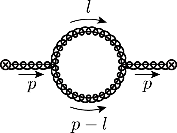
Figure 2: Assignment of the momenta for the final-state gluons.

The momentum of the jet is given by $p$, and the momenta of the two gluons are labeled as $l$ and $p-l$ respectively. Suppose that the jet is collinear in the $n$ lightcone direction. Then the momenta of the gluons can be written as

$$p_{1}=(l_{-},l_{\perp},l_{+}),\ p_{2}=(\omega-l_{-},-l_{\perp},p^{2}/\omega-l_{+}),$$ (27)

where $\omega=\overline{n}\cdot p=p_{-}$. The energies of the gluons and the invariant mass squared of the jet are given by

$$E_{1}=\frac{1}{2}(l_{-}+l_{+}),\ \ E_{2}=\frac{1}{2}(\omega-l_{-}+\frac{p^{2}}{\omega}-l_{+}),\ p^{2}=\frac{\omega l_{+}}{1-l_{-}/\omega}.$$ (28)

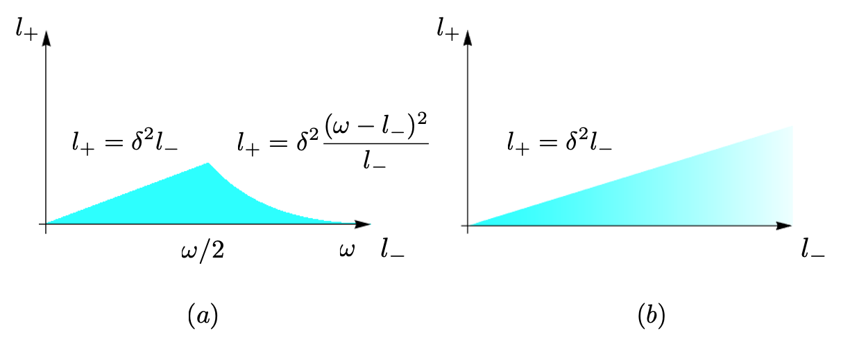
Figure 3: Phase space for the $n$-collinear jet function. (a) Naive collinear contribution, (b) Zero-bin contribution in the limit $l_{-}\rightarrow 0$. Another limit $l_{-}\rightarrow\omega$ gives the same result.

The cone jet algorithm for the $n$-collinear jet requires $\theta_{1}<R$ and $\theta_{2}<R$, where $R$ is the jet cone size, and $\theta_{i}$ is the angle of the gluon $i$ with respect to the jet axis, which is chosen to be in the $n$ direction. This jet algorithm for the collinear part can be written as Chay et al. (2015a); Cheung et al. (2009); Ellis et al. (2010)

$$\Theta_{J}=\Theta\Bigl{(}\delta^{2}>\frac{l_{+}}{l_{-}}\Bigr{)}\Theta\Bigl{(}l_{-}<\frac{\omega}{2}\Bigr{)}+\Theta\Bigl{(}\delta^{2}>\frac{l_{-}l_{+}}{(\omega-l_{-})^{2}}\Bigr{)}\Theta\Bigl{(}l_{-}>\frac{\omega}{2}\Bigr{)},$$ (29)

where $\delta=\tan R/2$. The two final-state particles should satisfy both $\theta_{1}<R$ and $\theta_{2}<R$. However, if $E_{1}<E_{2}$, that is, if $l_{-}<\omega/2$, when the constraint $\theta_{1}<R$ is satisfied, the condition $\theta_{2}<R$ is automatically satisfied, and vice versa. This fact is implemented in the jet algorithm, Eq. (29). The above jet algorithm includes the soft modes when $l_{-}\rightarrow 0$ for $p_{1}$ or $l_{-}\rightarrow\omega$ for $p_{2}$. The zero-bin subtraction should be employed to subtract the soft contribution from the jet function to avoid double counting Manohar and Stewart (2007). If we switch $p_{1}$ and $p_{2}$ in Eq. (29), the two terms are switched to give the same result. And the calculation involved in the jet function is also invariant under this switch since the final-state particles are identical. Therefore the zero-bin contribution is obtained by choosing the jet algorithm for the zero-bin contribution from the first term in Eq. (29) with $l_{-}\rightarrow 0$, and we multiply it by two to get the final answer. Therefore the jet algorithm for the zero-bin contribution is given by

$$\Theta_{J}^{0}=\Theta\Bigl{(}\delta^{2}>\frac{l_{+}}{l_{-}}\Bigr{)}.$$ (30)

The phase spaces for the naive collinear contribution and the zero-bin contribution are shown in Fig. 3 (a), (b) respectively. Here we consider the integrated gluon jet function $\mathcal{J}_{g}$.

The Feynman diagrams for the gluon jet function at one loop are shown in Fig. 4. Figs. 4 (a) and (b) are the virtual and real corrections from the Wilson lines. Figs. 4 (c)–(e) are the cut diagrams for a fermion, a gluon and a ghost loop respectively. The vertical dashed lines represent the unitarity cuts. We present the result by including the modified Wilson lines in Eq. (III) to extract the rapidity divergence.

The naive collinear and zero-bin contributions from Fig. 4 (a) are given as

$$\tilde{M}_{a} =\frac{ig^{2}C_{A}}{2}\Bigl{(}\frac{\mu^{2}e^{\gamma}}{4\pi}\Bigr{)}^{\epsilon}\int\frac{d^{D}l}{(2\pi)^{D}}\frac{1}{l^{2}(p-l)^{2}}\Bigl{[}\frac{\omega+l_{-}}{\omega-l_{-}}\Bigl{(}\frac{\nu}{\omega-l_{-}}\Bigr{)}^{\eta}+\frac{2\omega-l_{-}}{l_{-}}\Bigl{(}\frac{\nu}{l_{-}}\Bigr{)}^{\eta}\Bigr{]}$$

$$=-\frac{\alpha_{s}C_{A}}{4\pi}\Bigl{(}\frac{1}{\epsilon_{\mathrm{UV}}}-\frac{1}{\epsilon_{\mathrm{IR}}}\Bigr{)}\int_{0}^{\omega}dl_{-}\frac{2\omega-l_{-}}{l_{-}}\Bigl{(}\frac{\nu}{l_{-}}\Bigr{)}^{\eta},$$ (31)

$$M_{a}^{\varnothing} =-2ig^{2}C_{A}\Bigl{(}\frac{\mu^{2}e^{\gamma}}{4\pi}\Bigr{)}^{\epsilon}\int\frac{d^{D}l}{(2\pi)^{D}}\frac{1}{l^{2}l_{-}l_{+}}\Bigl{(}\frac{\nu}{l_{-}}\Bigr{)}^{\eta}=-\frac{\alpha_{s}C_{A}}{4\pi}\Bigl{(}\frac{1}{\epsilon_{\mathrm{UV}}}-\frac{1}{\epsilon_{\mathrm{IR}}}\Bigr{)}\int_{0}^{\infty}dl_{-}\frac{2\omega}{l_{-}}\Bigl{(}\frac{\nu}{l_{-}}\Bigr{)}^{\eta},$$

where $\omega=p^{-}$, and the contour integral in the complex $l_{+}$-plane is performed first. Here we use the relation

$$\mu^{2\epsilon}\int_{0}^{\infty}\frac{d\mathbf{l}_{\perp}^{2}}{(\mathbf{l}_{\perp}^{2})^{1+\epsilon}}=\frac{1}{\epsilon_{\mathrm{UV}}}-\frac{1}{\epsilon_{\mathrm{IR}}}.$$ (32)

The net contribution is given as

$$M_{a} =\tilde{M}_{a}-M_{a}^{\varnothing}=-\frac{\alpha_{s}C_{A}}{4\pi}\Bigl{(}\frac{1}{\epsilon_{\mathrm{UV}}}-\frac{1}{\epsilon_{\mathrm{IR}}}\Bigr{)}\Bigl{[}\int_{0}^{1}dx(-1)-\int_{1}^{\infty}dx2x^{-1-\eta}\Bigr{]}$$

$$=\frac{\alpha_{s}C_{A}}{4\pi}\Bigl{(}\frac{1}{\epsilon_{\mathrm{UV}}}-\frac{1}{\epsilon_{\mathrm{IR}}}\Bigr{)}\Bigl{(}\frac{2}{\eta}+2\ln\frac{\nu}{\omega}+1\Bigr{)},$$ (33)

where $x=l_{-}/\omega$. The zero-bin contribution is divided to extract the rapidity divergence, and it comes from the integration of $x$ in the interval $[1,\infty]$. The spurious divergence at $x=0$ is cancelled when we perform the zero-bin subtraction.

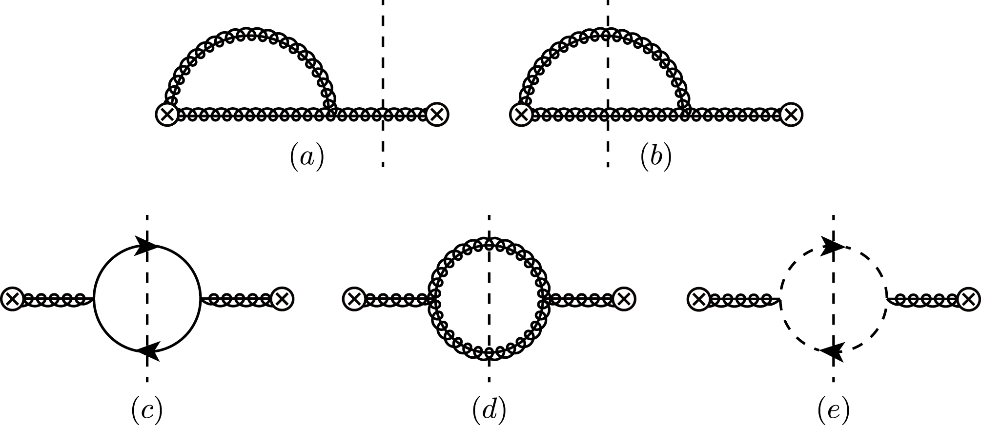
Figure 4: Feynman diagrams for the gluon jet function. Curly lines are gluons, solid lines with arrows are fermions, dashed lines with arrows are ghost particles. The vertical dashed lines represent the unitarity cut. (a) Virtual correction (b) real gluon emission, and the mirror images are omitted. The remainder represents the contributions from the cuts of (c) a fermion loop (d) a gluon loop and (e) a ghost loop. The diagrams for the wave function renormalization are not shown here.

The naive collinear contribution from Fig. 4 (b) is given by

$$\tilde{M}_{b} =\frac{\alpha_{s}C_{A}}{8\pi\omega}\frac{(\mu^{2}e^{\gamma_{\mathrm{E}}})^{\epsilon}}{\Gamma(1-\epsilon)}\int dl_{-}dl_{+}l_{+}^{-1-\epsilon}l_{-}^{-\epsilon}\Bigl{(}\frac{\nu}{l_{-}}\Bigr{)}^{\eta}\Bigl{(}\frac{\omega+l_{-}}{\omega-l_{-}}+\frac{2\omega-l_{-}}{l_{-}}\Bigr{)}\Theta_{J}$$

$$=\frac{\alpha_{s}C_{A}}{4\pi}\Bigl{[}\frac{1}{\epsilon_{\mathrm{IR}}^{2}}+\frac{1}{\epsilon_{\mathrm{IR}}}\Bigl{(}1+\ln\frac{\mu^{2}}{\omega^{2}\delta^{2}}\Bigr{)}+\ln\frac{\mu^{2}}{\omega^{2}\delta^{2}}+\frac{1}{2}\ln^{2}\frac{\mu^{2}}{\omega^{2}\delta^{2}}+2+2\ln 2-\frac{5}{12}\pi^{2}\Bigr{]}.$$ (34)

Note that there is no rapidity divergence in the naive contribution. The zero-bin contribution, using Eq. (30), is given as

$$M_{b}^{\varnothing} =\frac{\alpha_{s}C_{A}}{2\pi}\frac{(\mu^{2}e^{\gamma_{\mathrm{E}}})^{\epsilon}}{\Gamma(1-\epsilon)}\int_{0}^{\infty}dl_{-}l_{-}^{-1-\epsilon}\Bigl{(}\frac{\nu}{l_{-}}\Bigr{)}^{\eta}\int_{0}^{\delta^{2}l_{-}}dl_{+}l_{+}^{-1-\epsilon}$$

$$=\frac{\alpha_{s}C_{A}}{2\pi}\frac{e^{\gamma_{\mathrm{E}}\epsilon}}{\Gamma(1-\epsilon)}\Bigl{(}\frac{\mu^{2}}{\omega^{2}}\Bigr{)}^{\epsilon}\Bigl{(}\frac{\nu}{\omega}\Bigr{)}^{\eta}\int_{0}^{\infty}dxx^{-1-\epsilon-\eta}\int_{0}^{\delta^{2}x}dyy^{-1-\epsilon},$$ (35)

where we rescale the variables as $x=l_{-}/\omega$, $y=l_{+}/\omega$. If we integrate the above integral by brute force, the $y$-integral produces an IR pole $1/\epsilon_{\mathrm{IR}}$, and the $x$-integral reaches the infinity which cannot be handled by $\epsilon_{\mathrm{IR}}$. Therefore care must be taken to compute this integral. The $x$-integral is divided into two regions with an arbitrary number $\kappa$ as

$$I =\int_{0}^{\infty}dxx^{-1-\epsilon-\eta}\int_{0}^{\delta^{2}x}dyy^{-1-\epsilon}=\Bigl{[}\int_{0}^{\kappa}dxx^{-1-\epsilon-\eta}+\int_{\kappa}^{\infty}dxx^{-1-\epsilon-\eta}\Bigr{]}\int_{0}^{\delta^{2}x}dyy^{-1-\epsilon}$$

$$=\int_{0}^{\kappa}dxx^{-1-\epsilon-\eta}\int_{0}^{\delta^{2}x}dyy^{-1-\epsilon}+\int_{\kappa}^{\infty}dxx^{-1-\epsilon-\eta}\Bigl{[}\int_{0}^{\infty}dyy^{-1-\epsilon}-\int_{\delta^{2}x}^{\infty}dyy^{-1-\epsilon}\Bigr{]}$$ (36)

$$=\int_{0}^{\kappa}dxx^{-1-\epsilon}\int_{0}^{\delta^{2}x}dyy^{-1-\epsilon}-\int_{\kappa}^{\infty}dxx^{-1-\epsilon}\int_{\delta^{2}x}^{\infty}dyy^{-1-\epsilon}+\int_{\kappa}^{\infty}dxx^{-1-\epsilon-\eta}\int_{0}^{\infty}dyy^{-1-\epsilon}.$$

The first integral contains the IR divergence only, and it can be expressed in terms of the poles in $\epsilon_{\mathrm{IR}}$. Similarly, the second integral is of pure UV origin, and it can be expressed in terms of $\epsilon_{\mathrm{UV}}$. They do not contain any rapidity divergence. The last integral involves a rapidity divergence because the phase space contains the region $x\rightarrow\infty$ and $y\rightarrow 0$, and it can be evaluated by changing variables to $\alpha^{2}=xy$ and $\beta^{2}=y/x$. Then the third integral is given as

$$\int_{0}^{\infty}d\alpha^{2}(\alpha^{2})^{-1-\epsilon-\eta/2}\int_{0}^{\alpha/\kappa}d\beta\beta^{-1+\eta}=\frac{\kappa^{-\eta}}{\eta}\Bigl{(}\frac{1}{\epsilon_{\mathrm{UV}}}-\frac{1}{\epsilon_{\mathrm{IR}}}\Bigr{)}.$$ (37)

When all the terms are added in Eq. (V.1), the dependence on an arbitrary $\kappa$ cancels and the zero-bin contribution is given by

$$M_{b}^{\varnothing}=\frac{\alpha_{s}C_{A}}{4\pi}\Bigl{[}-\frac{1}{\epsilon_{\mathrm{UV}}^{2}}+\frac{1}{\epsilon_{\mathrm{IR}}^{2}}+\Bigl{(}\frac{1}{\epsilon_{\mathrm{UV}}}-\frac{1}{\epsilon_{\mathrm{IR}}}\Bigr{)}\Bigl{(}\frac{2}{\eta}+\ln\frac{\nu^{2}\delta^{2}}{\mu^{2}}\Bigr{)},\Bigr{]},$$ (38)

and the net contribution is given as

$$M_{b}=\tilde{M}_{b}-M_{b}^{\varnothing} =\frac{\alpha_{s}C_{A}}{4\pi}\Bigl{[}\frac{1}{\epsilon_{\mathrm{UV}}^{2}}-\frac{1}{\epsilon_{\mathrm{UV}}}\Bigl{(}\frac{2}{\eta}+\ln\frac{\nu^{2}\delta^{2}}{\mu^{2}}\Bigr{)}+\frac{1}{\epsilon_{\mathrm{IR}}}\Bigl{(}1+\frac{2}{\eta}+2\ln\frac{\nu}{\omega}\Bigr{)}$$

$$+\ln\frac{\mu^{2}}{\omega^{2}\delta^{2}}+\frac{1}{2}\ln^{2}\frac{\mu^{2}}{\omega^{2}\delta^{2}}+2+2\ln 2-\frac{5}{12}\pi^{2}\Bigr{]}.$$ (39)

If we add $M_{a}$ and $M_{b}$, we obtain the result

$$M_{a}+M_{b}=\frac{\alpha_{s}C_{A}}{4\pi}\Bigl{[}\frac{1}{\epsilon_{\mathrm{UV}}^{2}}+\frac{1}{\epsilon_{\mathrm{UV}}}\Bigl{(}1+\ln\frac{\mu^{2}}{\omega^{2}\delta^{2}}\Bigr{)}+\ln\frac{\mu^{2}}{\omega^{2}\delta^{2}}+\frac{1}{2}\ln^{2}\frac{\mu^{2}}{\omega^{2}\delta^{2}}+2+2\ln 2-\frac{5}{12}\pi^{2}\Bigr{]},$$ (40)

which is free of the IR and the rapidity divergences.

The loops in Figs. 4 (c)-(e) consist of fermions, gluons and ghost particles respectively. The zero-bin contributions are power suppressed compared to the naive collinear contributions, thus neglected. The naive collinear contributions from the fermions, the gluons and the ghost particles are given respectively by

$$\tilde{M}_{f} =\frac{\alpha_{s}T_{F}n_{f}}{2\pi\omega}\frac{(\mu^{2}e^{\gamma_{\mathrm{E}}})^{\epsilon}}{\Gamma(1-\epsilon)}\int dl_{-}dl_{+}l_{-}^{2-\epsilon}\Bigl{(}1-\frac{l_{-}}{\omega}\Bigr{)}^{2}l_{+}^{-1-\epsilon}\Bigl{[}\Bigl{(}\frac{1}{l_{-}}+\frac{1}{\omega-l_{-}}\Bigr{)}^{2}-\frac{2}{1-\epsilon}\frac{1}{l_{-}(\omega-l_{-})}\Bigr{]}\Theta_{J}$$

$$=\frac{\alpha_{s}T_{F}n_{f}}{4\pi}\Bigl{(}-\frac{4}{3\epsilon_{\mathrm{IR}}}-\frac{4}{3}\ln\frac{\mu^{2}}{\omega^{2}\delta^{2}}-\frac{23}{9}-\frac{8}{3}\ln 2\Bigr{)},$$

$$\tilde{M}_{g} =-\frac{\alpha_{s}C_{A}}{8\pi\omega}\frac{(\mu^{2}e^{\gamma_{\mathrm{E}}})^{\epsilon}}{\Gamma(1-\epsilon)}\int dl_{-}dl_{+}\Bigl{[}4l_{-}^{-\epsilon}l_{+}^{-1-\epsilon}-\frac{5-4\epsilon}{1-\epsilon}l_{-}^{1-\epsilon}\Bigl{(}1-\frac{l_{-}}{\omega}\Bigr{)}\frac{l_{+}^{-1-\epsilon}}{\omega}\Bigr{]}\Theta_{J}$$

$$=\frac{\alpha_{s}C_{A}}{8\pi}\Bigl{(}\frac{19}{6\epsilon_{\mathrm{IR}}}+\frac{19}{6}\ln\frac{\mu^{2}}{\omega^{2}\delta^{2}}+\frac{247}{36}+\frac{19}{3}\ln 2\Bigr{)},$$

$$\tilde{M}_{\mathrm{ghost}} =-\frac{\alpha_{s}C_{A}}{8\pi\omega^{2}}\frac{(\mu^{2}e^{\gamma_{\mathrm{E}}})^{\epsilon}}{\Gamma(1-\epsilon)}\int dl_{-}dl_{+}l_{-}^{1-\epsilon}\Bigl{(}1-\frac{l_{-}}{\omega}\Bigr{)}l_{+}^{-1-\epsilon}\Theta_{J}$$

$$=\frac{\alpha_{s}C_{A}}{8\pi}\Bigl{(}\frac{1}{6\epsilon_{\mathrm{IR}}}+\frac{1}{6}\ln\frac{\mu^{2}}{\omega^{2}\delta^{2}}+\frac{13}{36}+\frac{1}{3}\ln 2\Bigr{)},$$ (41)

where $n_{f}$ is the number of quark flavors. The total contribution is given by

$$\tilde{M}_{f}+\tilde{M}_{g}+\tilde{M}_{\mathrm{ghost}} =\frac{\alpha_{s}}{4\pi}\Bigl{[}\Bigl{(}\frac{5}{3}C_{A}-\frac{4}{3}T_{F}n_{f}\Bigr{)}\Bigl{(}\frac{1}{\epsilon_{\mathrm{IR}}}+\ln\frac{\mu^{2}}{\omega^{2}\delta^{2}}\Bigr{)}$$

$$+\frac{65}{18}C_{A}-\frac{23}{9}T_{F}n_{f}+2\Bigl{(}\frac{5}{3}C_{A}-\frac{4}{3}T_{F}n_{f}\Bigr{)}\ln 2\Bigr{]}.$$ (42)

Finally, the gluon field-strength renormalization at one loop is given by

$$Z_{g}^{(1)}=\frac{\alpha_{s}}{4\pi}\Bigl{(}\frac{1}{\epsilon_{\mathrm{UV}}}-\frac{1}{\epsilon_{\mathrm{IR}}}\Bigr{)}\Bigl{(}\frac{5}{3}C_{A}-\frac{4}{3}T_{F}n_{f}\Bigr{)}.$$ (43)

The overall contribution of the real and virtual corrections from the gluon self energy at order $\alpha_{s}$ is given by

$$M_{\mathrm{self}} =\frac{\alpha_{s}}{4\pi}\Bigl{[}\Bigl{(}\frac{5}{3}C_{A}-\frac{4}{3}T_{F}n_{f}\Bigr{)}\Bigl{(}\frac{1}{\epsilon_{\mathrm{UV}}}+\ln\frac{\mu^{2}}{\omega^{2}\delta^{2}}\Bigr{)}$$

$$+\frac{65}{18}C_{A}-\frac{23}{9}T_{F}n_{f}+2\Bigl{(}\frac{5}{3}C_{A}-\frac{4}{3}T_{F}n_{f}\Bigr{)}\ln 2\Bigr{]}.$$ (44)

The total collinear contributions are given by

$$M_{\mathrm{coll}} =2(M_{a}+M_{b})+M_{\mathrm{self}}$$

$$=\frac{\alpha_{s}}{2\pi}\Bigl{[}\frac{C_{A}}{\epsilon_{\mathrm{UV}}^{2}}+\frac{1}{\epsilon_{\mathrm{UV}}}\Bigl{(}\frac{\beta_{0}}{2}+C_{A}\ln\frac{\mu^{2}}{\omega^{2}\delta^{2}}\Bigr{)}+\frac{\beta_{0}}{2}\ln\frac{\mu^{2}}{\omega^{2}\delta^{2}}+\frac{1}{2}C_{A}\ln^{2}\frac{\mu^{2}}{\omega^{2}\delta^{2}}$$

$$+\frac{137}{36}C_{A}-\frac{23}{18}T_{F}n_{f}+\beta_{0}\ln 2-\frac{5}{12}C_{A}\pi^{2}\Bigr{]},$$ (45)

where $\beta_{0}=11C_{A}/3-4T_{F}n_{f}/3$ is the leading term of the QCD beta function. [See Eq. (102).] The collinear contribution is clearly IR finite, and the renormalized gluon jet function at one loop is obtained by adding the counterterms as

$$\mathcal{J}_{g}^{(1)}(\omega\delta,\mu)=\frac{\alpha_{s}}{4\pi}\Bigl{(}\beta_{0}\ln\frac{\mu^{2}}{\omega^{2}\delta^{2}}+C_{A}\ln^{2}\frac{\mu^{2}}{\omega^{2}\delta^{2}}+\frac{137}{18}C_{A}-\frac{23}{9}T_{F}n_{f}+2\beta_{0}\ln 2-\frac{5}{6}C_{A}\pi^{2}\Bigr{)}.$$ (46)

This coincides with the result on the unmeasured gluon jet function obtained in Ref. Ellis et al. (2010). And the anomalous dimension of the gluon jet function at NLO is given by

$$\gamma_{J}=\frac{d}{d\ln\mu}\mathcal{J}_{g}=\frac{\alpha_{s}}{\pi}\Bigl{(}C_{A}\ln\frac{\mu^{2}}{\omega^{2}\delta^{2}}+\frac{\beta_{0}}{2}\Bigr{)}.$$ (47)

V.2 Quark beam function

The beam jets are produced in the beam directions from the initial-state radiation, and the evolution of the initial-state particles from $Q\lambda$ to $\mu$ is described by the beam function. The quark beam function and the unmeasured quark beam function are defined in Eqs. (12) and (13), and we compute the unmeasured quark beam function here. The Feynman diagrams for the beam functions at one loop are shown in Fig. 5. Fig. 5 (a) is the virtual correction, Fig. 5 (b) and (c) are real gluon emissions.

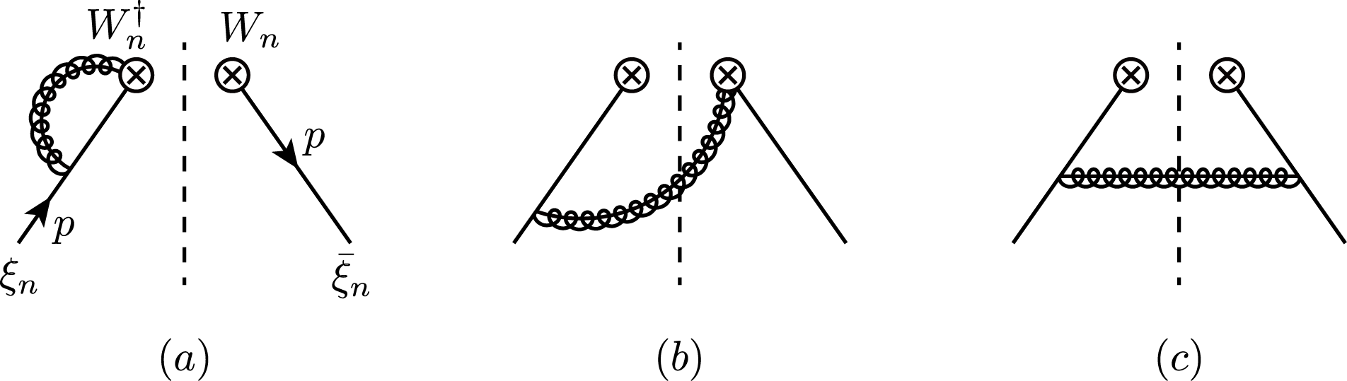
Figure 5: Feynman diagrams for the $n$-collinear beam function at one loop (a) virtual corrections, (b) and (c) real gluon emission. The mirror images of (a) and (b) are omitted. the dashed lines denote the final-state cuts.

The naive collinear contribution from Fig. 5 (a) is given as

$$\tilde{M}_{a} =2ig^{2}C_{F}\Bigl{(}\frac{\mu^{2}e^{\gamma}}{4\pi}\Bigr{)}^{\epsilon}\delta(1-z)\int\frac{d^{D}l}{(2\pi)^{D}}\frac{\omega-l_{-}}{l^{2}(l-p)^{2}l_{-}}\Bigl{(}\frac{\nu}{l_{-}}\Bigr{)}^{\eta}$$

$$=-\frac{\alpha_{s}C_{F}}{2\pi}\Bigl{(}\frac{\nu}{\omega}\Bigr{)}^{\eta}\delta(1-z)\Bigl{(}\frac{1}{\epsilon_{\mathrm{UV}}}-\frac{1}{\epsilon_{\mathrm{IR}}}\Bigr{)}\int_{0}^{1}dx\frac{1-x}{x^{1+\eta}},$$ (48)

where $x=l_{-}/\omega$. There is unwanted divergence as $x\rightarrow 0$, but it is cancelled by the zero-bin contribution which is given as

$$M_{a}^{\varnothing}=-\frac{\alpha_{s}C_{F}}{2\pi}\Bigl{(}\frac{\nu}{\omega}\Bigr{)}^{\eta}\delta(1-z)\Bigl{(}\frac{1}{\epsilon_{\mathrm{UV}}}-\frac{1}{\epsilon_{\mathrm{IR}}}\Bigr{)}\int_{0}^{\infty}dx\frac{1}{x^{1+\eta}}.$$ (49)

As in the calculation of the beam function, the net collinear contribution from Fig. 5 (a) is given by

$$M_{a}=\tilde{M}_{a}-M_{a}^{\varnothing}=\frac{\alpha_{s}C_{F}}{2\pi}\delta(1-z)\Bigl{(}\frac{1}{\epsilon_{\mathrm{UV}}}-\frac{1}{\epsilon_{\mathrm{IR}}}\Bigr{)}\Bigl{(}\frac{1}{\eta}+\ln\frac{\nu}{\omega}+1\Bigr{)}.$$ (50)

The naive contribution from Fig. 5 (b) is written as

$$\tilde{M}_{b} =-4\pi g^{2}C_{F}\Bigl{(}\frac{\mu^{2}e^{\gamma}}{4\pi}\Bigr{)}^{\epsilon}\int dt\int\frac{d^{D}l}{(2\pi)^{D}}\frac{\omega-l_{-}}{(l-p)^{2}l_{-}}\Bigl{(}\frac{\nu}{l_{-}}\Bigr{)}^{\eta}\delta(l^{2})\delta\Bigl{(}1-z-\frac{l_{-}}{\omega}\Bigr{)}\delta(t-\omega l_{+})\Theta_{B}$$

$$=\frac{\alpha_{s}C_{F}}{2\pi}\Bigl{(}\frac{\nu}{\omega}\Bigr{)}^{\eta}\frac{(\mu^{2}e^{\gamma_{\mathrm{E}}})^{\epsilon}}{\Gamma(1-\epsilon)}\int_{0}^{z(1-z)\delta^{2}\omega^{2}}dt\,t^{-1-\epsilon}z^{1+\epsilon}(1-z)^{-1-\epsilon-\eta}.$$ (51)

We treat $\eta$ much smaller than $\epsilon$, hence $\eta$ can be neglected. Then $\tilde{M}_{b}$ can be written as

$$\tilde{M}_{b}=-\frac{\alpha_{s}C_{F}}{2\pi}\frac{(\mu^{2}e^{\gamma_{\mathrm{E}}})^{\epsilon}}{\Gamma(1-\epsilon)}\frac{1}{\epsilon_{\mathrm{IR}}}(\delta^{2}\omega^{2})^{-\epsilon}z(1-z)^{-1-2\epsilon}.$$ (52)

Here we use the relation

$$(1-z)^{-1-2\epsilon}=-\frac{1}{2\epsilon_{\mathrm{IR}}}\delta(1-z)+\mathcal{L}_{0}(1-z)-2\epsilon_{\mathrm{IR}}\mathcal{L}_{1}(1-z)+\cdots,$$ (53)

where the functions $\mathcal{L}_{n}(z)$ are defined as

$$\mathcal{L}_{n}(z)\equiv\Bigl{[}\frac{\theta(z)\ln^{n}z}{z}\Bigr{]}_{+}=\lim_{\beta\rightarrow 0}\Bigl{[}\frac{\theta(z-\beta)\ln^{n}z}{z}+\delta(z-\beta)\frac{\ln^{n+1}\beta}{n+1}\Bigr{]}.$$ (54)

Then the naive contribution contains only the IR divergence and is given by

$$\tilde{M}_{b} =\frac{\alpha_{s}C_{F}}{2\pi}\Bigl{[}\Bigl{(}\frac{1}{2\epsilon_{\mathrm{IR}}^{2}}+\frac{1}{2\epsilon_{\mathrm{IR}}}\ln\frac{\mu^{2}}{\omega^{2}\delta^{2}}+\frac{1}{4}\ln^{2}\frac{\mu^{2}}{\omega^{2}\delta^{2}}-\frac{\pi^{2}}{24}\Bigr{)}\delta(1-z)$$

$$-\frac{1}{\epsilon_{\mathrm{IR}}}z\mathcal{L}_{0}(1-z)-z\mathcal{L}_{0}(1-z)\ln\frac{\mu^{2}}{\omega^{2}\delta^{2}}+2z\mathcal{L}_{1}(1-z)\Bigr{]}.$$ (55)

The zero-bin contribution $M_{b}^{\varnothing}$ is written as

$$M_{b}^{\varnothing} =\frac{\alpha_{s}C_{F}}{2\pi}\frac{(\mu^{2}e^{\gamma_{\mathrm{E}}})^{\epsilon}}{\Gamma(1-\epsilon)}\int dl_{+}dl_{-}\frac{1}{(l_{+}l_{-})^{1+\epsilon}}\Bigl{(}\frac{\nu}{l_{-}}\Bigr{)}^{\eta}\Theta_{B}$$

$$=\frac{\alpha_{s}C_{F}}{2\pi}\frac{e^{\gamma\epsilon}}{\Gamma(1-\epsilon)}\Bigl{(}\frac{\mu^{2}}{\omega^{2}}\Bigr{)}^{\epsilon}\Bigl{(}\frac{\nu}{\omega}\Bigr{)}^{\eta}\int_{0}^{\infty}dx\,x^{-1-\epsilon-\eta}\int_{0}^{\delta^{2}x}dy\,y^{-1-\epsilon}$$

$$=\frac{\alpha_{s}C_{F}}{2\pi}\delta(1-z)\Bigl{[}-\frac{1}{2}\Bigl{(}\frac{1}{\epsilon_{\mathrm{UV}}^{2}}-\frac{1}{\epsilon_{\mathrm{IR}}^{2}}\Bigr{)}+\frac{1}{2}\Bigl{(}\frac{1}{\epsilon_{\mathrm{UV}}}-\frac{1}{\epsilon_{\mathrm{IR}}}\Bigr{)}\Bigl{(}\frac{2}{\eta}+\ln\frac{\nu^{2}\delta^{2}}{\mu^{2}}\Bigr{)}\Bigr{]}.$$ (56)

The net contribution is given by

$$M_{b} =\tilde{M}_{b}-M_{b}^{\varnothing}$$

$$=\frac{\alpha_{s}C_{F}}{2\pi}\Bigl{\{}\delta(1-z)\Bigl{[}\frac{1}{2\epsilon_{\mathrm{UV}}^{2}}+\frac{1}{2\epsilon_{\mathrm{UV}}}\ln\frac{\mu^{2}}{\omega^{2}\delta^{2}}+\frac{1}{4}\ln^{2}\frac{\mu^{2}}{\omega^{2}\delta^{2}}-\Bigl{(}\frac{1}{\epsilon_{\mathrm{UV}}}-\frac{1}{\epsilon_{\mathrm{IR}}}\Bigr{)}\Bigl{(}\frac{1}{\eta}+\ln\frac{\nu}{\omega}-\frac{\pi^{2}}{24}\Bigr{)}\Bigr{]}$$

$$-\Bigl{(}\frac{1}{\epsilon_{\mathrm{IR}}}+\ln\frac{\mu^{2}}{\omega^{2}\delta^{2}}\Bigr{)}z\mathcal{L}_{0}(1-z)+2z\mathcal{L}_{1}(1-z)\Bigr{\}}.$$ (57)

The contribution of Fig. 5 (c) is given as

$$M_{c} =4\pi g^{2}C_{F}(1-\epsilon)\Bigl{(}\frac{\mu^{2}e^{\gamma_{\mathrm{E}}}}{4\pi}\Bigr{)}^{\epsilon}\int dt\int\frac{d^{D}{l}}{(2\pi)^{D}}\frac{\mathbf{l}_{\perp}^{2}}{[(l-p)^{2}]^{2}}\delta(l^{2})\delta(t-\omega l_{+})\omega\delta(\omega-p_{-}+l_{-})$$

$$=-\frac{\alpha_{s}C_{F}}{2\pi}(1-z)\Bigl{(}\frac{1}{\epsilon_{\mathrm{IR}}}-1+\ln\frac{\mu^{2}}{\omega^{2}\delta^{2}}-2\ln(1-z)\Bigr{)}.$$ (58)

The zero-bin contribution is suppressed and is neglected.

By including the wave function renormalization, the beam function at NLO is given by

$$B^{(1)}(z,\delta,\mu)=2(M_{a}+M_{b})+M_{c}-\frac{\alpha_{s}C_{F}}{4\pi}\delta(1-z)\Bigl{(}\frac{1}{\epsilon_{\mathrm{UV}}}-\frac{1}{\epsilon_{\mathrm{IR}}}\Bigr{)}$$ (59)

$$=\frac{\alpha_{s}C_{F}}{2\pi}\Bigl{\{}\delta(1-z)\Bigl{[}\frac{1}{\epsilon_{\mathrm{UV}}^{2}}+\frac{1}{\epsilon_{\mathrm{UV}}}\Bigl{(}\ln\frac{\mu^{2}}{\omega^{2}\delta^{2}}+\frac{3}{2}\Bigr{)}+\frac{1}{2}\ln^{2}\frac{\mu^{2}}{\omega^{2}\delta^{2}}+\frac{3}{2}\ln\frac{\mu^{2}}{\omega^{2}\delta^{2}}-\frac{\pi^{2}}{12}\Bigr{]}$$

$$-P_{qq}(z)\Bigl{(}\frac{1}{\epsilon_{\mathrm{IR}}}+\ln\frac{\mu^{2}}{\omega^{2}\delta^{2}}\Bigr{)}+4z\mathcal{L}_{1}(1-z)+(1-z)\Bigl{(}1+2\ln(1-z)\Bigr{)}\Bigr{\}},$$

where $P_{qq}(z)$ is the splitting function, which is defined as

$$P_{qq}(z)=\frac{3}{2}\delta(1-z)+2z\mathcal{L}_{0}(1-z)+(1-z).$$ (60)

Note that the beam function contains the IR divergence, which is the same as the PDF, and it is absorbed into the nonperturbative matrix element in the beam function in exactly the same way as we treat the PDF.

The renormalized beam function at NLO by removing the divergent terms is given by

$$B_{R}^{(1)}(z,\omega\delta,\mu)=\frac{\alpha_{s}C_{F}}{2\pi}\Bigl{(}\frac{1}{2}\ln^{2}\frac{\mu^{2}}{\omega^{2}\delta^{2}}+\frac{3}{2}\ln\frac{\mu^{2}}{\omega^{2}\delta^{2}}+8-\frac{3}{4}\pi^{2}\Bigr{)},$$ (61)

and the anomalous dimension of the beam function at NLO is given as

$$\gamma_{B}^{(1)}=\mu\frac{d}{d\mu}B^{(1)}=\frac{\alpha_{s}}{\pi}\ln\frac{\mu^{2}}{\omega^{2}\delta^{2}}+\frac{\alpha_{s}}{\pi}\frac{3}{2}C_{F}.$$ (62)

VI Soft function

The soft function, defined in Eq. (15), is given again by

$$S_{JI}=\sum_{X_{s}}\mathrm{tr}\langle 0|Y_{1}^{\dagger}(\mathcal{Y}_{3}^{\dagger}T_{J}^{\dagger}\mathcal{Y}_{4})^{ba}Y_{2}|X_{s}\rangle\Theta_{J}\Theta_{B}\langle X_{s}|Y_{2}^{\dagger}(\mathcal{Y}_{4}^{\dagger}T_{I}\mathcal{Y}_{3})^{ab}Y_{1}|0\rangle.$$ (63)

The Wilson lines $Y_{2}^{\dagger}$ and $Y_{1}$ correctly describe the soft gluon emission from the antiquark and the quark in the initial state. But, to be exact, the Wilson lines $\mathcal{Y}_{4}^{\dagger}$ and $\mathcal{Y}_{3}$ should be $\tilde{\mathcal{Y}}_{4}^{\dagger}$ and $\tilde{\mathcal{Y}}_{3}$, describing the soft gluon emission from the outgoing particles Chay et al. (2005). However, we keep the forms as they are for notational simplicity. The soft Wilson lines are given as

$$Y_{1}=\sum_{\mathrm{perm.}}\exp\Bigl{[}\frac{1}{n_{1}\cdot\mathcal{R}+i0}(-gn_{1}\cdot A_{s})\Bigr{]},\ Y_{2}^{\dagger}=\sum_{\mathrm{perm.}}\exp\Bigl{[}-gn_{2}\cdot A_{s}\frac{1}{n_{2}\cdot\mathcal{R}^{\dagger}-i0}\Bigr{]},$$

$$\mathcal{Y}_{3}=\sum_{\mathrm{perm.}}\exp\Bigl{[}\frac{1}{n_{3}\cdot\mathcal{R}-i0}(-gn_{3}\cdot A_{s})\Bigr{]},\ \mathcal{Y}_{4}^{\dagger}=\sum_{\mathrm{perm.}}\exp\Bigl{[}-gn_{4}\cdot A_{s}\frac{1}{n_{4}\cdot\mathcal{R}^{\dagger}+i0}\Bigr{]},$$ (64)

where $\mathcal{R}$ is the operator extracting the soft momentum. The rapidity regulator cannot be expressed in a general form, and it will be presented in the explicit calculation order by order.

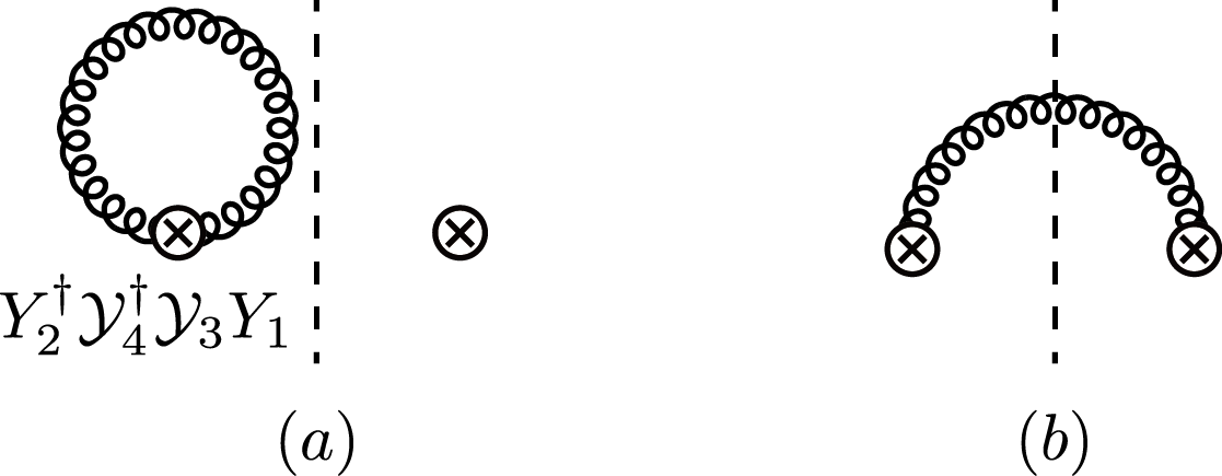
Figure 6: Feynman diagrams for the soft function at one loop. (a) Virtual correction (b) Real gluon emission. The hermitian conjugates are omitted. The dashed lines are the unitarity cuts.

The Feynman diagrams for the soft function at NLO is shown in Fig. 6. Figs. 6 (a) and (b) represent the virtual and the real corrections respectively. The vertical dashed lines are the unitarity cuts, and the hermitian conjugates are not shown. Fig. 6 (a) yields

$$M_{ij}^{V}=-2\pi g^{2}\Bigl{(}\frac{\mu^{2}e^{\gamma_{\mathrm{E}}}}{4\pi}\Bigr{)}^{\epsilon}\int\frac{d^{D}{l}}{(2\pi)^{D}}\frac{2n_{ij}}{l_{i}l_{j}}\delta(l^{2})R(l_{i},l_{j}),$$ (65)

apart from the group theory factors $-\mathbf{T}_{i}\cdot\mathbf{T}_{j}$ Chiu et al. (2009); Catani and Seymour (1996, 1997). Here $n_{ij}=n_{i}\cdot n_{j}/2$, $l_{i}=n_{i}\cdot l$ and $l_{j}=n_{j}\cdot l$. $R(l_{i},l_{j})$ is the rapidity regulator, which can be written at order $\alpha_{s}$ as

$$R(l_{i},l_{j})=\Bigl{(}\frac{\nu n_{ij}}{l_{i}}\Bigr{)}^{\eta}\theta(l_{i}-l_{j})+\Bigl{(}\frac{\nu n_{ij}}{l_{j}}\Bigr{)}^{\eta}\theta(l_{j}-l_{i}).$$ (66)

In the basis of $n_{i}$ and $n_{j}$, the momentum $l_{i}^{\mu}$ can be written as

$$l^{\mu}=l_{j}\frac{n_{i}^{\mu}}{2n_{ij}}+l_{i}\frac{n_{j}^{\mu}}{2n_{ij}}+l_{ij,\perp}^{\mu},$$ (67)

where $l_{ij,\perp}^{\mu}$ is the momentum perpendicular to $n_{i}$ and $n_{j}$, with $l^{2}=l_{i}l_{j}/n_{ij}+l_{ij,\perp}^{2}$.

Since Eq. (65) is symmetric under the exchange $i\leftrightarrow j$, we pick up the first part of the rapidity regulator in Eq. (66) and multiply two. Then the virtual contribution is given as

$$M_{ij}^{V} =-\frac{\alpha_{s}}{\pi}\frac{(\mu^{2}e^{\gamma_{\mathrm{E}}})^{\epsilon}}{\Gamma(1-\epsilon)}\int dl_{i}dl_{j}\Bigl{(}\frac{l_{i}l_{j}}{n_{ij}}\Bigr{)}^{-\epsilon}\frac{1}{l_{i}l_{j}}\Bigl{(}\frac{n_{ij}\nu}{l_{i}}\Bigr{)}^{\eta}\theta(l_{i}>l_{j})$$

$$=-\frac{\alpha_{s}}{\pi}\frac{(\mu^{2}e^{\gamma_{\mathrm{E}}})^{\epsilon}}{\Gamma(1-\epsilon)}n_{ij}^{\epsilon+\eta}\nu^{\eta}\int_{0}^{\infty}dl_{i}l_{i}^{-1-\epsilon-\eta}\int_{0}^{l_{i}}dl_{j}l_{j}^{-1-\epsilon}.$$ (68)

In order to extract the divergences correctly, we separate the integration regions by introducing an arbitrary intermediate scale $\Omega$ as

$$I =\int_{0}^{\infty}dl_{i}l_{i}^{-1-\epsilon-\eta}\int_{0}^{l_{i}}dl_{j}l_{j}^{-1-\epsilon}$$

$$=\int_{0}^{\Omega}dl_{i}l_{i}^{-1-\epsilon-\eta}\int_{0}^{l_{i}}dl_{j}l_{j}^{-1-\epsilon}+\int_{\Omega}^{\infty}dl_{i}l_{i}^{-1-\epsilon-\eta}\Big{[}\int_{0}^{\infty}dl_{j}l_{j}^{-1-\epsilon}-\int_{l_{i}}^{\infty}dl_{j}l_{j}^{-1-\epsilon}\Bigr{]}.$$ (69)

The first (third) term yields the IR (UV) divergence, and the second term is computed by changing variables $l_{i}l_{j}=\alpha^{2}$ and $l_{j}/l_{i}=\beta^{2}$ to extract the rapidity divergence. The overall result is independent of $\Omega$, and the result is given by

$$M_{ij}^{V}=\frac{\alpha_{s}}{2\pi}\Bigl{[}\frac{1}{\epsilon_{\mathrm{UV}}^{2}}-\frac{1}{\epsilon_{\mathrm{IR}}^{2}}+\Bigl{(}\frac{1}{\epsilon_{\mathrm{UV}}}-\frac{1}{\epsilon_{\mathrm{IR}}}\Bigr{)}\Bigl{(}-\frac{2}{\eta}+\ln\frac{\mu^{2}}{\nu^{2}n_{ij}}\Bigr{)}\Bigr{]}.$$ (70)

The jet algorithm and the veto should be applied to the real gluon emission. The main contribution comes from the configuration in which the gluon is emitted from the soft Wilson lines with the eikonal factor $1/n_{i}\cdot l$ or $1/n_{j}\cdot l$ and the jet algorithm or the beam veto is applied with respect to the $n_{i}$ or $n_{j}$ direction. We will denote these contributions as $M_{ij,i}^{R}$ and $M_{ij,j}^{R}$ respectively. The contribution $M_{ij,k}^{R}$, in which the $n_{k}$ direction is neither $n_{i}$ nor $n_{j}$, is not correlated to the $n_{k}$ direction, hence it is proportional to the area of the jet cone, $\delta^{2}$, and is neglected.

The real contribution from the jet algorithm is given as

$$M_{ij,i}^{R}=2\pi g^{2}\Bigl{(}\frac{\mu^{2}e^{\gamma_{\mathrm{E}}}}{4\pi}\Bigr{)}^{\epsilon}\int\frac{d^{D}{l}}{(2\pi)^{D}}\frac{2n_{ij}}{n_{i}\cdot ln_{j}\cdot l}\delta(l^{2})\Bigl{(}\frac{\nu}{\overline{n}_{i}\cdot l}\Bigr{)}^{\eta}\Theta(n_{i}\cdot l<\delta_{i}^{2}\overline{n}_{i}\cdot l)\Theta(l^{0}>\Lambda),$$ (71)

where the rapidity regulator is written as $(\nu/\overline{n}_{i}\cdot l)^{\eta}$ because the soft gluon is in the collinear region due to the jet algorithm. For the same reason, $n_{j}\cdot l$ can be expressed as

$$n_{j}\cdot l=n_{j}\cdot\Bigl{(}\overline{n}_{i}\cdot l\frac{n_{i}}{2}+l_{i\perp}+n_{i}\cdot l\frac{\overline{n}_{i}}{2}\Bigr{)}\approx n_{ij}\overline{n}_{i}\cdot l.$$ (72)

Here the size of the jet cone in the $n_{i}$ direction is denoted as $\delta_{i}$ to distinguish the jet radius ($i=3,4$) and the beam veto ($i=1,2$) with $\delta_{1,2}=e^{-y_{\mathrm{cut}}}$. Then, by writing $\overline{n}_{i}\cdot l=l_{-}$ and $n_{i}\cdot l=l_{+}$, $M_{ij,i}^{R}$ is written as

$$M_{ij,i}^{R} =\frac{\alpha_{s}}{2\pi}\frac{(\mu^{2}e^{\gamma_{\mathrm{E}}})^{\epsilon}}{\Gamma(1-\epsilon)}\nu^{\eta}\int dl_{-}dl_{+}l_{-}^{-1-\epsilon-\eta}l_{+}^{-1-\epsilon}\Theta(l_{+}<l_{-}\delta_{i}^{2})\Theta(l_{-}>2\Lambda)$$

$$=\frac{\alpha_{s}}{2\pi}\frac{(\mu^{2}e^{\gamma_{\mathrm{E}}})^{\epsilon}}{\Gamma(1-\epsilon)}\nu^{\eta}\int_{2\Lambda}^{\infty}dl_{-}l_{-}^{-1-\epsilon-\eta}\int_{0}^{\delta_{i}^{2}l_{-}}dl_{+}l_{+}^{-1-\epsilon}$$

$$=\frac{\alpha_{s}}{2\pi}\Bigl{[}\Bigl{(}\frac{1}{\epsilon_{\mathrm{UV}}}-\frac{1}{\epsilon_{\mathrm{IR}}}\Bigr{)}\Bigl{(}\frac{1}{\eta}+\ln\frac{\nu}{2\Lambda}\Bigr{)}-\frac{1}{2\epsilon_{\mathrm{UV}}^{2}}-\frac{1}{\epsilon_{\mathrm{UV}}}\ln\frac{\mu}{2\Lambda\delta_{i}}-\ln^{2}\frac{\mu}{2\Lambda\delta_{i}}\Bigr{]}.$$ (73)

The contribution of $M_{ij,k}^{R}$ can be written as

$$M_{ij,k}^{R}=2\pi g^{2}\Bigl{(}\frac{\mu^{2}e^{\gamma_{\mathrm{E}}}}{4\pi}\Bigr{)}^{\epsilon}\int\frac{d^{D}{l}}{(2\pi)^{D}}\frac{2n_{ij}}{n_{i}\cdot ln_{j}\cdot l}\delta(l^{2})\Theta(n_{k}\cdot l<\delta_{k}^{2}\overline{n}_{k}\cdot l)\Theta(\overline{n}_{k}\cdot l>2\Lambda).$$ (74)

Because there is no rapidity divergence in the integral, the rapidity regulator is absent. Since the gluon momentum is $n_{k}$-collinear, $n_{i}\cdot l$ and $n_{j}\cdot l$ can be written as

$$n_{i}\cdot l\approx n_{i}\cdot\frac{n_{k}}{2}\overline{n}_{k}\cdot l=n_{ik}l_{-},\ \ n_{j}\cdot l\approx n_{jk}l_{-},$$ (75)

where $l_{-}=\overline{n}_{k}\cdot l$. Then $M_{ij,k}^{R}$ is given as

$$M_{ij,k}^{R} =\frac{\alpha_{s}}{2\pi}\frac{n_{ij}}{n_{ik}n_{jk}}\frac{(\mu^{2}e^{\gamma_{\mathrm{E}}})^{\epsilon}}{\Gamma(1-\epsilon)}\int dl_{-}dl_{+}\frac{(l_{-}l_{+})^{-\epsilon}}{l_{-}^{2}}\Theta(l_{+}<\delta_{k}^{2}l_{-})\Theta(l_{-}>2\Lambda)$$

$$=\frac{\alpha_{s}}{2\pi}\frac{n_{ij}}{n_{ik}n_{jk}}\frac{(\mu^{2}e^{\gamma_{\mathrm{E}}})^{\epsilon}}{\Gamma(1-\epsilon)}\int_{2\Lambda}^{\infty}dl_{-}(l_{-})^{-2-\epsilon}\int_{0}^{\delta_{k}^{2}l_{-}}dl_{+}(l_{+})^{-\epsilon}$$

$$=\frac{\alpha_{s}}{4\pi}\frac{n_{ij}}{n_{ik}n_{jk}}\delta_{k}^{2}\Bigl{(}\frac{1}{\epsilon_{\mathrm{UV}}}+1+2\ln\frac{\mu}{2\Lambda}-\ln\delta_{k}^{2}\Bigr{)}.$$ (76)

As claimed before, it is proportional to $\delta_{k}^{2}$ and is neglected.

The soft part $M_{ij}^{\mathrm{veto}}$ is given by

$$M_{ij}^{\mathrm{veto}}=g^{2}\Bigl{(}\frac{\mu^{2}e^{\gamma}}{4\pi}\Bigr{)}^{\epsilon}\int\frac{d^{D}l}{(2\pi)^{D}}\frac{n_{i}\cdot n_{j}}{n_{i}\cdot ln_{j}\cdot l}2\pi\delta(l^{2})\Theta(l_{0}<\Lambda).$$ (77)

The integration can be performed by choosing the lightcone vectors as

$$n_{i}=(1,0,0,1),\ \ n_{j}=(1,\sin\theta,0,\cos\theta),$$ (78)

We can express the momentum $l^{\mu}$ in the $r_{i}$ basis as

$$l^{\mu}=l_{0}r_{0}^{\mu}+l_{1}r_{1}^{\mu}+l_{3}r_{3}^{\mu}+l_{\perp}^{\mu},$$ (79)

where $r_{0}^{\mu}=(1,0,\mathbf{0},0)$, $r_{1}^{\mu}=(0,1,\mathbf{0},0)$, $r_{3}^{\mu}=(0,0,\mathbf{0},1)$, and $l_{\perp}^{\mu}$ is perpendicular to $r_{i}$. The point of choosing these bases is that $n_{i}\cdot l$ and $n_{j}\cdot l$ have nonzero components in the 0, 1 and 3 directions. And all the other components reside in the $1-2\epsilon$ dimensions, which we call the perpendicular direction. The integration measure $d^{D}l$ can be written as

$$d^{D}l=dl_{0}dl_{1}dl_{3}d^{1-2\epsilon}\mathbf{l}_{\perp}=dl_{0}dl_{1}dl_{3}d\mathbf{l}^{2}_{\perp}(\mathbf{l}^{2}_{\perp})^{1/2-\epsilon}\frac{d\Omega_{1-2\epsilon}}{2}=\frac{\pi^{1/2-\epsilon}}{\Gamma(\frac{1}{2}-\epsilon)}dl_{0}dl_{1}dl_{3}d\mathbf{l}^{2}_{\perp}(\mathbf{l}^{2}_{\perp})^{1/2-\epsilon},$$ (80)

where the angular integral over $\Omega_{1-2\epsilon}$ is performed.

The soft part $M_{ij}^{\mathrm{veto}}$ is written as

$$M_{ij}^{\mathrm{veto}} =\frac{\alpha_{s}}{2\pi}\frac{(e^{\gamma_{\mathrm{E}}}\mu^{2})^{\epsilon}}{\sqrt{\pi}\Gamma(\frac{1}{2}-\epsilon)}\int dl_{0}dl_{1}dl_{3}d\mathbf{l}^{2}_{\perp}(\mathbf{l}^{2}_{\perp})^{1/2-\epsilon}\frac{1-\cos\theta}{(l_{0}-l_{3})(l_{0}-l_{3}\cos\theta-l_{1}\sin\theta)}$$

$$\times\delta(l_{0}^{2}-l_{1}^{2}-l_{3}^{2}-\mathbf{l}_{\perp}^{2})\theta(l_{0})\theta(\Lambda-l_{0})$$

$$=\frac{\alpha_{s}}{2\pi}\frac{(e^{\gamma_{\mathrm{E}}}\mu^{2})^{\epsilon}}{\sqrt{\pi}\Gamma(\frac{1}{2}-\epsilon)}\int dl_{0}dl_{1}dl_{3}\frac{(1-\cos\theta)(l_{0}^{2}-l_{1}^{2}-l_{3}^{2})^{-1/2-\epsilon}}{(l_{0}-l_{3})(l_{0}-l_{3}\cos\theta-l_{1}\sin\theta)}\theta(l_{0})\theta(\Lambda-l_{0})$$ (81)

Now we change the variables $l_{3}=l_{0}k\cos\phi$ and $l_{1}=l_{0}\sin\phi$ with $dl_{0}dl_{3}dl_{1}=dl_{0}dkd\phi kl_{0}^{2}$ to write $M_{ij}^{\mathrm{veto}}$ as

$$M_{ij}^{\mathrm{veto}} =\frac{\alpha_{s}}{2\pi}\frac{(e^{\gamma_{\mathrm{E}}}\mu^{2})^{\epsilon}}{\sqrt{\pi}\Gamma(\frac{1}{2}-\epsilon)}\int_{0}^{\Lambda}dl_{0}l_{0}^{-1-2\epsilon}\int_{0}^{1}dkk(1-k^{2})^{-1/2-\epsilon}\int_{0}^{2\pi}\frac{d\phi}{(1-k\cos\phi)(1-\cos(\phi-\theta))}$$

$$=\frac{\alpha_{s}(1-\cos\theta)}{\sqrt{\pi}}\frac{(e^{\gamma_{\mathrm{E}}}\mu^{2})^{\epsilon}}{\sqrt{\pi}\Gamma(\frac{1}{2}-\epsilon)}\int_{0}^{\Lambda}dl_{0}l_{0}^{-1-2\epsilon}\int_{0}^{1}dk\frac{k(1-k^{2})^{-1-\epsilon}}{1-k^{2}(1+\cos\theta)/2}$$

$$=\frac{\alpha_{s}}{2\pi}\Bigl{(}\frac{1}{\epsilon_{\mathrm{IR}}^{2}}+\frac{1}{\epsilon_{\mathrm{IR}}}\ln\frac{\mu^{2}}{4n_{ij}\Lambda^{2}}+\frac{1}{2}\ln^{2}\frac{\mu^{2}}{4n_{ij}\Lambda^{2}}+Li_{2}(1-n_{ij})-\frac{\pi^{2}}{4}\Bigr{)}.$$ (82)

The total soft contribution at next-to-leading order is given by

$$S_{ij} =M_{ij}^{V}+M_{ij,i}^{R}+M_{ij,j}^{R}+M_{ij}^{\mathrm{veto}}$$

$$=\frac{\alpha_{s}}{2\pi}\Bigl{(}\frac{1}{\epsilon_{\mathrm{UV}}}\ln\frac{\delta_{i}\delta_{j}}{n_{ij}}+2\ln\frac{\mu}{2\Lambda}\ln\frac{\delta_{i}\delta_{j}}{n_{ij}}-\ln^{2}\delta_{i}-\ln^{2}\delta_{j}+Li_{2}(1-n_{ij})-\frac{\pi^{2}}{4}\Bigr{)}.$$ (83)

The soft function is given by $-\sum_{i,j}\mathbf{T}_{i}\cdot\mathbf{T}_{j}S_{ij}$, and it can be written as a matrix in the operator basis.

VII Evolution of the scattering cross section

The dijet cross section is written as

$$\sigma =\frac{1}{64\pi N_{c}^{2}S^{2}}\sum_{IJ}\int dtH_{IJ}(\mu)S_{JI}(\mu)\int\frac{dz_{1}}{z_{1}}B_{q/N_{1}}(z_{1},E_{\mathrm{cm}}e^{-y_{cut}},\mu)$$

$$\times\int\frac{dz_{2}}{z_{2}}B_{\bar{q}/N_{2}}(z_{2},E_{\mathrm{cm}}e^{-y_{cut}},\mu)\mathcal{J}_{g_{3}}(\omega_{3}\delta_{3},\mu)\mathcal{J}_{g_{4}}(\omega_{4}\delta_{4},\mu).$$ (84)

The cross section is the product of the hard function $H_{IJ}$, the soft function $S_{JI}$, the jet functions and the beam functions. Each function starts from the characteristic scales $\mu_{i}$, at which the logarithms become small, and scales to the common factorization scale $\mu_{F}$. The characteristic scales are given as $\mu_{H}\sim\omega$ for the hard part, $\mu_{J}\sim\omega\delta$ and $\mu_{B}\sim\omega\delta$ for the collinear parts, and $\mu_{S}\sim\Lambda$ for the soft part. The overall cross section is independent of the factorization scale $\mu_{F}$. The evolution of each component in the jet cross section can be obtained by solving the RG equations.

VII.1 The hard function

The hard function is given by $H_{IJ}=C_{I}C_{J}^{*}$, where $C_{I}$ is the Wilson coefficient of $O_{I}$ obtained by the matching between the full QCD and SCET. The detailed form of the hard function at one loop for $2\rightarrow 2$ partonic processes can be found in Ref. Kelley and Schwartz (2011). The relation between the bare and the renormalized hard functions is given by

$$\mathbf{H}_{\mathrm{bare}}=\mathbf{Z}_{H}(\mu)\mathbf{H}(\mu)\mathbf{Z}_{H}^{\dagger}(\mu),$$ (85)

and the renormalization group equation for the hard function is given by

$$\frac{d}{d\ln\mu}\mathbf{H}=\mathbf{\Gamma}_{H}\mathbf{H}+\mathbf{H}\mathbf{\Gamma}_{H}^{\dagger},$$ (86)

where the anomalous dimension matrix $\mathbf{\Gamma}_{H}$ is defined as

$$\mathbf{\Gamma}_{H}=-\mathbf{Z}_{H}^{-1}\frac{d}{d\ln\mu}\mathbf{Z}_{H}.$$ (87)

The anomalous dimension matrix $\mathbf{\Gamma}_{H}$ can be written as Kelley and Schwartz (2011); Hornig et al. (2016)

$$\mathbf{\Gamma}_{H}=\sum_{i=1}^{4}\Bigl{[}\frac{C_{i}}{2}\Gamma_{c}(\alpha_{s})\ln\frac{-t}{\mu^{2}}+\gamma_{i}\Bigr{]}\mathbf{1}+\Gamma_{c}(\alpha_{s})\mathbf{M}_{H},$$ (88)

where $\Gamma_{c}(\alpha_{s})$ is the cusp anomalous dimension which can be expanded as Korchemsky and Radyushkin (1987)

$$\Gamma_{c}(\alpha_{s})=\frac{\alpha_{s}}{4\pi}\Gamma_{c}^{0}+\Bigl{(}\frac{\alpha_{s}}{4\pi}\Bigr{)}^{2}\Gamma_{c}^{1}+\cdots,$$ (89)

with

$$\Gamma_{c}^{0}=4,\ \Gamma_{c}^{1}=\Bigl{(}\frac{268}{9}-\frac{4}{3}\pi^{2}\Bigr{)}C_{A}-\frac{40n_{f}}{9}.$$ (90)

To NLL accuracy, the cusp anomalous dimension to two loops is needed. The Casimir invariants $C_{i}$ are given by $C_{q}=C_{F}$, $C_{g}=C_{A}$, and $\gamma_{i}$ are given by

$$\gamma_{q}=-\frac{\alpha_{s}}{2\pi}\frac{3}{2}C_{F},\ \gamma_{g}=-\frac{\alpha_{s}}{2\pi}\frac{\beta_{0}}{2}.$$ (91)

The matrix $\mathbf{M}_{H}$ can be written as

$$\mathbf{M}_{H}=-\sum_{i<j}\mathbf{T}_{i}\cdot\mathbf{T}_{j}\Bigl{[}L(s_{ij})-L(t)\Bigr{]},$$ (92)

where $s_{ij}$ are given as

$$s=s_{12}=(p_{1}+p_{2})^{2}=n_{12}\omega_{1}\omega_{2}=s_{34}=(p_{3}+p_{4})^{2}=n_{34}\omega_{3}\omega_{4},$$

$$t=s_{13}=(p_{1}-p_{3})^{2}=-n_{13}\omega_{1}\omega_{3}=s_{24}=(p_{2}-p_{4})^{2}=-n_{24}\omega_{2}\omega_{4},$$

$$u=s_{14}=(p_{1}-p_{4})^{2}=-n_{14}\omega_{1}\omega_{4}=s_{23}=(p_{2}-p_{3})^{2}=-n_{23}\omega_{2}\omega_{3}.$$ (93)

And

$$L(t)=\ln\frac{-t}{\mu^{2}},\ L(u)=\ln\frac{-u}{\mu^{2}},\ L(s)=\ln\frac{s}{\mu^{2}}-i\pi.$$ (94)

Specifically, for $q\overline{q}\rightarrow gg$, the first part of $\mathbf{\Gamma}_{H}$ proportional to the identity matrix in Eq. (88) is written as

$$\frac{\alpha_{s}}{2\pi}\Bigl{[}C_{H}\ln\frac{n_{13}\omega_{1}\omega_{3}}{\mu^{2}}-3C_{F}-\beta_{0}\Bigr{]}\mathbf{1}=\Bigl{[}\Gamma_{c}\frac{C_{H}}{2}\ln\frac{n_{13}\omega_{1}\omega_{3}}{\mu^{2}}-2\gamma_{g}-2\gamma_{q}\Bigr{]}\mathbf{1},$$ (95)

where $C_{H}=n_{q}C_{F}+n_{g}C_{A}=2C_{F}+2C_{A}$. And the nondiagonal part $\mathbf{M}_{H}$ is given as

$$\mathbf{M}_{H} =\begin{pmatrix}\displaystyle\frac{C_{F}}{2}\ln\frac{n_{12}n_{34}}{n_{13}n_{24}}&0&\displaystyle\ln\frac{n_{13}n_{24}}{n_{14}n_{23}}\\ 0&\displaystyle\frac{C_{F}}{2}\ln\frac{n_{12}n_{34}}{n_{13}n_{24}}+\frac{C_{A}}{2}\ln\frac{n_{14}n_{23}}{n_{13}n_{24}}&\displaystyle\ln\frac{n_{14}n_{23}}{n_{13}n_{24}}\\ \displaystyle\frac{1}{4}\ln\frac{n_{12}n_{34}}{n_{14}n_{23}}&\displaystyle\frac{1}{4}\ln\frac{n_{12}n_{34}}{n_{13}n_{24}}&\displaystyle\frac{C_{F}+C_{A}}{2}\ln\frac{n_{12}n_{34}}{n_{13}n_{24}}\end{pmatrix}-i\pi\mathbf{T},$$ (96)

where $\mathbf{T}$ is given by

$$\mathbf{T}=\begin{pmatrix}C_{F}&0&0\\ 0&C_{F}&0\\ 1/2&1/2&C_{F}+C_{A}\end{pmatrix}.$$ (97)

The imaginary part $-i\pi\mathbf{T}$ in $\mathbf{M}$ does not contribute to the evolution, and the solution to RG equation, Eq. (86), is written as

$$\mathbf{H}(\mu_{F})=\Pi_{H}(\mu_{F},\mu_{H})\bm{\Pi}_{H}(\mu_{F},\mu_{H})\mathbf{H}(\mu_{H})\bm{\Pi}^{\dagger}_{H}(\mu_{F},\mu_{H}),$$ (98)

where $\Pi_{H}$, and $\bm{\Pi}_{H}$ are given by

$$\Pi_{H}(\mu_{F},\mu_{H}) =\exp\Bigl{[}-2C_{H}S_{\Gamma}(\mu_{F},\mu_{H})-C_{H}a_{\Gamma}(\mu_{F},\mu_{H})\ln\frac{\mu_{H}^{2}}{-t}$$

$$+4a_{\gamma_{q}}(\mu_{F},\mu_{H})+4a_{\gamma_{g}}(\mu_{F},\mu_{H})\Bigr{]},$$

$$\bm{\Pi}_{H}(\mu_{F},\mu_{H}) =\exp\Bigl{[}a_{\Gamma}(\mu_{F},\mu_{H})\mathbf{M}_{H}\Bigr{]}.$$ (99)

Here $\Pi_{H}$ is the evolution kernal from the identity matrix in $\bm{\Gamma}_{H}$, and $\bm{\Pi}_{H}$ is the evolution from the matrix $\mathbf{M}_{H}$.

The quantities in Eq. (VII.1) are defined as

$$S_{\Gamma}(\mu,\mu_{i})=\int_{\alpha(\mu_{i})}^{\alpha(\mu)}d\alpha\frac{\Gamma_{\mathrm{cusp}}(\alpha)}{\beta(\alpha)}\int_{\alpha(\mu_{i})}^{\alpha}\frac{d\alpha^{\prime}}{\beta(\alpha^{\prime})},\ \ \ a_{f}(\mu,\mu_{i})=\int_{\alpha(\mu_{i})}^{\alpha(\mu)}\frac{d\alpha}{\beta(\alpha)}f(\alpha),$$ (100)

where $f(\alpha)$ is a function of $\alpha$. The beta function $\beta(\alpha_{s})$ is defined as

$$\beta(\alpha_{s})=\mu\frac{d\alpha_{s}}{d\mu}=-2\alpha_{s}\Bigl{[}\beta_{0}\Bigl{(}\frac{\alpha_{s}}{4\pi}\Bigr{)}+\beta_{1}\Bigl{(}\frac{\alpha_{s}}{4\pi}\Bigr{)}^{2}+\cdots\Bigr{]},$$ (101)

where

$$\beta_{0}=\frac{11}{3}C_{A}-\frac{4}{3}T_{F}n_{f},\ \ \beta_{1}=\frac{34}{3}C_{A}^{2}-\frac{20}{3}C_{A}T_{F}n_{f}-4C_{F}T_{F}n_{f}.$$ (102)

VII.2 The beam function

The RG equation for the beam function is written as

$$\frac{d}{d\ln\mu}B_{i}(z_{i},\delta_{i}\omega_{i},\mu)=\gamma_{B_{i}}(\mu)B_{i}(z_{i},\delta_{i}\omega_{i},\mu),$$ (103)

where the anomalous dimension for the beam function is given by

$$\gamma_{B_{i}}(\mu)=2C_{F}\Gamma_{c}\ln\frac{\mu}{\delta_{i}\omega_{i}}-2\gamma_{q}.$$ (104)

The solution of the RG equation is written as

$$B_{i}(z_{i},\delta_{i}\omega_{i},\mu_{F})=U_{B_{i}}(\mu_{F},\mu_{B})\mathcal{B}_{i}(z_{i},\delta_{i}\omega_{i},\mu_{B}),$$ (105)

where the evolution kernel $U_{B}$ is given by

$$U_{B_{i}}(\mu_{F},\mu_{B})=\exp\Bigl{[}2C_{F}S_{\Gamma}(\mu_{F},\mu_{B})+2C_{F}a_{\Gamma}(\mu_{F},\mu_{B})\ln\frac{\mu_{B}}{\delta_{i}\omega_{i}}-2a_{\gamma_{q}}(\mu_{F},\mu_{B})\Bigr{]}.$$ (106)

VII.3 The jet function

The RG equation for the jet function is written as

$$\frac{d}{d\ln\mu}\mathcal{J}_{g_{i}}(\omega_{i}\delta_{i},\mu)=\gamma_{J_{i}}\mathcal{J}_{g_{i}}(\omega_{i}\delta_{i},\mu),$$ (107)

where the anomalous dimension $\gamma_{J_{i}}$ is given by

$$\gamma_{J_{i}}=2C_{A}\Gamma_{c}\ln\frac{\mu}{\delta_{i}\omega_{i}}-2\gamma_{g}.$$ (108)

The evolution of the jet function is given by

$$\mathcal{J}_{g_{i}}(\omega_{i}\delta_{i},\mu_{F})=U_{J_{i}}(\mu_{F},\mu_{J})\mathcal{J}_{g_{i}}(\omega_{i}\delta_{i},\mu_{J}),$$ (109)

where the evolution kernel $U_{J_{i}}$ is given as

$$U_{J_{i}}(\mu_{F},\mu_{J})=\exp\Bigl{[}2C_{A}S_{\Gamma}(\mu_{F},\mu_{J})+2C_{A}a_{\Gamma}(\mu_{F},\mu_{J})\ln\frac{\mu_{J}}{\delta_{i}\omega_{i}}-2a_{\gamma_{g}}(\mu_{F},\mu_{J})\Bigr{]}.$$ (110)

VII.4 The soft function

The soft function is renormalized in a matrix form as

$$\mathbf{S}_{\mathrm{bare}}=\mathbf{Z}_{S}^{\dagger}(\mu)\mathbf{S}(\mu)\mathbf{Z}_{S}(\mu),$$ (111)

and the RG equation is given as

$$\frac{d}{d\ln\mu}\mathbf{S}=\mathbf{S}\mathbf{\Gamma}_{S}+\mathbf{\Gamma}_{S}^{\dagger}\mathbf{S},$$ (112)

where the anomalous dimension matrix $\mathbf{\Gamma}_{S}$ is defined as

$$\mathbf{\Gamma}_{S}=-\Bigl{(}\frac{d}{d\ln\mu}\mathbf{Z}_{S}\Bigr{)}\mathbf{Z}_{S}^{-1}.$$ (113)

The soft contribution $S_{ij}$ is given by Eq. (VI), from which the anomalous soft dimensions can be obtained. Let us define $U_{ij}$ by

$$\frac{\Gamma_{c}}{2}U_{ij}\equiv\frac{dS_{ij}}{d\ln\mu}=\Gamma_{c}\ln\frac{\delta_{i}\delta_{j}}{n_{ij}}.$$ (114)

Then the anomalous dimension matrix of the soft function is given as

$$\mathbf{\Gamma}_{S}=\Gamma_{c}\Bigl{(}-\frac{1}{2}\sum_{i<j}\mathbf{T}_{i}\cdot\mathbf{T}_{j}U^{S}_{ij}+i\pi\mathbf{T}\Bigr{)},$$ (115)

which can be written as

$$\bm{\Gamma}_{S}=\Bigl{(}C_{F}\Gamma_{c}\ln\frac{\delta_{1}\delta_{2}}{n_{12}}+C_{A}\Gamma_{c}\ln\frac{\delta_{3}\delta_{4}}{n_{34}}\Bigr{)}\mathbf{1}+\Gamma_{c}(\mathbf{M}_{S}+i\pi\mathbf{T}),$$ (116)

where $\mathbf{M}_{S}$ is given by

$$\mathbf{M}_{S}=\begin{pmatrix}\displaystyle\frac{C_{A}}{2}\ln\frac{n_{12}n_{34}}{n_{13}n_{24}}&0&\displaystyle\ln\frac{n_{14}n_{23}}{n_{13}n_{24}}\\ 0&\displaystyle\frac{C_{A}}{2}\ln\frac{n_{12}n_{34}}{n_{14}n_{23}}&\displaystyle\ln\frac{n_{13}n_{24}}{n_{14}n_{23}}\\ \displaystyle\frac{1}{4}\ln\frac{n_{14}n_{23}}{n_{12}n_{34}}&\displaystyle\frac{1}{4}\ln\frac{n_{13}n_{24}}{n_{12}n_{34}}&0\end{pmatrix},$$ (117)

and $\mathbf{T}$ is given by Eq. (97). We have inserted $\mathbf{T}$ to keep the consistency of the anomalous dimensions, and it does not affect Eq. (VII.5) below at one loop since $\mathbf{S}_{0}\mathbf{T}=\mathbf{T}^{\dagger}\mathbf{S}_{0}$, where $\mathbf{S}_{0}$ is the tree-level soft function.

The evolution of the soft function from the scale $\mu_{S}$ to the common factorization scale $\mu_{F}$ can be written as

$$\mathbf{S}(\mu_{F})=\Pi_{S}(\mu_{F},\mu_{S})\bm{\Pi}_{S}^{\dagger}(\mu_{F},\mu_{S})\mathbf{S}(\mu_{S})\bm{\Pi}_{S}(\mu_{F},\mu_{S}),$$ (118)

where the evolution kernels are given as

$$\Pi_{S}(\mu_{F},\mu_{S}) =\exp\Bigl{[}2C_{F}a_{\Gamma}(\mu_{F},\mu_{S})\ln\frac{\delta_{1}\delta_{2}}{n_{12}}+2C_{A}a_{\Gamma}(\mu_{F},\mu_{S})\ln\frac{\delta_{3}\delta_{4}}{n_{34}}\Bigr{]},$$

$$\bm{\Pi}_{S}(\mu_{F},\mu_{S}) =\exp\Bigl{[}a_{\Gamma}(\mu_{F},\mu_{S})\mathbf{M}_{S}\Bigr{]}.$$ (119)

The evolution kernel $\Pi_{S}$ is constructed from the diagonal part of the anomalous dimension matrix in Eq. (116), and $\bm{\Pi}_{S}$ from $\mathbf{M}_{S}$.

VII.5 Cancellation of the anomalous dimensions

The dijet cross section should be independent of the renormalization scale, which means that the sum of the anomalous dimensions of the factorized parts should be zero. Then the dijet cross section is independent of the factorization scale $\mu_{F}$. At NLO, the derivative of the dijet cross section in Eq. (VII) with respect to $\ln\mu$ yields

$$\frac{d\sigma}{d\ln\mu} =\Bigl{[}\mathrm{tr}\ \mathbf{H}_{0}\mathbf{S}_{0}\Bigl{(}\mathbf{\Gamma}_{H}+\mathbf{\Gamma}_{S}+\frac{1}{2}(\gamma_{B_{1}}+\gamma_{B_{2}}+\gamma_{J_{3}}+\gamma_{J_{4}})\mathbf{1}\Bigr{)}$$

$$+\mathrm{tr}\ \mathbf{S}_{0}\mathbf{H}_{0}\Bigl{(}\mathbf{\Gamma}_{H}^{\dagger}+\mathbf{\Gamma}_{S}^{\dagger}+\frac{1}{2}(\gamma_{B_{1}}+\gamma_{B_{2}}+\gamma_{J_{3}}+\gamma_{J_{4}})\mathbf{1}\Bigr{)}\Bigr{]}$$

$$\times\Bigl{(}B_{q/N_{1},0}B_{\bar{q}/N_{2},0}+(q\leftrightarrow\overline{q})\Bigr{)}\mathcal{J}_{g,0}\mathcal{J}_{g,0},$$ (120)

where the quantities with the subscript 0 are the tree-level quantities. The anomalous dimensions of the gluon jet function and the beam function are given by

$$\gamma_{B_{i}}=2C_{F}\Gamma_{c}\ln\frac{\mu}{\delta_{i}\omega_{i}}-2\gamma_{q},\ \ \gamma_{J_{i}}=2C_{A}\Gamma_{c}\ln\frac{\mu}{\delta_{i}\omega_{i}}-2\gamma_{g}.$$ (121)

From Eqs. (88), (115), the sum of the anomalous dimension matrices $\mathbf{\Gamma}_{H}+\mathbf{\Gamma}_{S}$ becomes diagonal and is given by

$$\mathbf{\Gamma}_{H}+\mathbf{\Gamma}_{S} =\Gamma_{c}\Bigl{[}\frac{C_{A}+C_{F}}{2}\ln\frac{n_{13}n_{24}\omega_{1}\omega_{2}\omega_{3}\omega_{4}}{\mu^{4}}+\frac{C_{A}+C_{F}}{2}\ln\frac{n_{12}n_{34}}{n_{13}n_{24}}$$

$$+C_{F}\ln\frac{\delta_{1}\delta_{2}}{n_{12}}+C_{A}\ln\frac{\delta_{3}\delta_{4}}{n_{34}}\Bigr{]}=-\frac{1}{2}\Bigl{(}\gamma_{B_{1}}+\gamma_{B_{2}}+\gamma_{J_{3}}+\gamma_{J_{4}}\Bigr{)}\mathbf{1},$$ (122)

where the second relation obtained using Eq. (VII.1). Therefore the total sum of the anomalous dimensions is given by

$$\mathbf{\Gamma}_{H}+\mathbf{\Gamma}_{S}+\frac{1}{2}\Bigl{(}\gamma_{B_{1}}+\gamma_{B_{2}}+\gamma_{J_{3}}+\gamma_{J_{4}}\Bigr{)}\mathbf{1}=0.$$ (123)

It is explicitly shown that the dijet cross section is independent of the renormalization scale $\mu$. Though the evolution kernels for each factorized part look complicated and depend on the factorization $\mu_{F}$ [See Eqs. (VII.1), (106), (110) and (VII.4).], the product of all the evolution kernels turn out to be independent of $\mu_{F}$.

VIII Conclusion

The factorization theorems for various physical observables ranging from the jet cross sections to more differential quantities such as the jet substructure are crucial in theoretical prediction. Once the factorization theorems are established, each factorized part depends on a single scale and its evolution can be computed using perturbation theory. When there are hierarchies of scales, as often happens in high-energy scattering, large logarithms of the ratio of disparate scales appear and they can be resummed using the RG equation. However, in order to resum the large logarithms, we have to ensure that the divergences are purely of the UV origin. Therefore the absence of the IR and rapidity divergences in each factorized part is vital in proving factorization theorems.

In this paper, we have considered the dijet cross section in hadron-hadron scattering by selecting a single partonic process $q\overline{q}\rightarrow gg$. We expect that the more differential the physical quantities we probe, the more complicated the proof of the factorization becomes. And this is just the starting point in that direction. Though the dijet cross section looks simple, it contains a lot of interesting physics as we delved deeper into the divergence structure in this paper.

We should emphasize that there are three issues which are not included here. Firstly, we have considered only the case in which the jet cone size is not small. By dissecting the phase space into the collinear and the soft regions, each factorized part is described by a single scale. For example, the characteristic scales are $\mu_{H}\sim\omega$, $\mu_{J}\sim\mu_{B}\sim\omega\delta$ and $\mu_{S}\sim\Lambda$ for the hard, collinear and soft scales respectively. The RG equation resums all the large logarithms when we scale from these scales to the factorization scale $\mu_{F}$. However, another large logarithm appears for small jet radius. The anomalous dimensions depend on the cone size, as can be seen in Eq. (47) for the jet function. In order to resum the large logarithms for the small radius, we decompose the phase space more appropriately including the so-called soft-collinear modes Dasgupta et al. (2015); Chien et al. (2016); Dasgupta et al. (2016). The large logarithm due to the small radius can be handled, but in this paper, we take a reasonable size of the jet radius $R\sim 0.7$ such that the small-radius resummation gives a very small effect.

Secondly, in proving the factorization theorem, the interaction of the Glauber gluons between the active partons and the spectator partons should be considered to ensure the factorization Bodwin (1985). We assume that the Glauber gluons do not violate the factorization, as in many other processes. And finally the issue of nonglobal logarithms should be raised, but if we choose appropriate observables such as the jettiness, the problem of the nonglobal logarithms can be avoided, though it should be considered at higher orders in the dijet cross section. In spite of these important issues, the factorization of the dijet cross section, the study of the divergence structure, and the resummation of large logarithms offer significant insights into the understanding of the hadron-hadron scattering.

We have also computed the anomalous dimensions of the hard, collinear and soft parts. The anomalous dimensions of the collinear quark beam functions and the gluon jet functions are diagonal, and those of the hard and soft functions are nontrivial matrices in the operator basis. The jet algorithm and the beam veto affect both the diagonal gluon jet functions, the beam functions, and the non-diagonal soft function. However, the dependence on the jet cone size in the soft function resides only in the diagonal part, and proportional to the identity matrix. This dependence of the jet cone radius in the soft function is cancelled by that in the beam and the jet functions. Also note that the nondiagonal part of the soft function in Eq. (117) has only directional dependences of $n_{ij}$. Interestingly enough, the nondiagonal part of the hard anomalous dimension matrix in Eq. (96) depends only on the directions, which cancel exactly that in the soft function. We have shown all these intertwined structure of the anomalous dimensions explicitly in the process $q\overline{q}\rightarrow gg$.

As already mentioned, the detailed analysis of extracting various divergences can be applied to other processes. It will be interesting to consider more differential observables probing jet substructure, such as angularity, $N$-jettiness, etc., and establish the factorization theorems and resum large logarithms. And as mentioned before, the issues of the small-$R$ resummation and the nonglobal logarithms will be pursued in the future.