Similarities and uniqueness of Ly$\boldsymbol{\alpha}$ emitters among star-forming galaxies at $\boldsymbol{z}$=2.5

Abstract

We conducted a deep narrow-band imaging survey with the Subaru Prime Focus Camera on the Subaru Telescope and constructed a sample of Ly$\alpha$ emitters (LAEs) at $z=2.53$ in the UDS-CANDELS field where a sample of H$\alpha$ emitters (HAEs) at the same redshift is already obtained from our previous narrow-band observation at NIR. The deep narrow-band and multi broadband data allow us to find LAEs of stellar masses and star-formation rates (SFRs) down to $\gtrsim$$10^{8}$ M_⊙ and $\gtrsim$0.2 M_⊙/yr, respectively. We show that the LAEs are located along the same mass-SFR sequence traced by normal star-forming galaxies such as HAEs, but towards a significantly lower mass regime. Likewise, LAEs seem to share the same mass–size relation with typical star-forming galaxies, except for the massive LAEs, which tend to show significantly compact sizes. We identify a vigorous mass growth in the central part of LAEs: the stellar mass density in the central region of LAEs increases as their total galaxy mass grows. On the other hand, we see no Ly$\alpha$ line in emission for most of the HAEs. Rather, we find that the Ly$\alpha$ feature is either absent or in absorption (Ly$\alpha$ absorbers; LAAs), and its absorption strength may increase with reddening of the UV continuum slope. We demonstrate that a deep Ly$\alpha$ narrow-band imaging like this study is able to search for not only LAEs but also LAAs in a certain redshift slice. This work suggests that LAEs trace normal star-forming galaxies in the low-mass regime, while they remain as a unique population because the majority of HAEs are not LAEs.

1 Introduction

The redshift interval of $z$=2.1–2.6 is the key epoch for us to understand the formation mechanisms of star-forming galaxies. In this era, the cosmic star-formation density is peaked (Hopkins & Beacom, 2006), galaxy morphology is still under construction (Papovich et al., 2005), and gaseous flows (feeding and feedback) are more prevalent compared to lower redshift counterparts (Yabe et al., 2015). Galaxies at this epoch allow us to study the physical origins of these processes based on their strong emission lines such as  H$\alpha$$\lambda 6563$,  [Oiii]$\lambda 5007$,  [Oii]$\lambda 3727$, and  Ly$\alpha$$\lambda 1216$ with the optical and near-infrared imagers and spectrographs. For example, we can directly investigate the physical properties of  Ly$\alpha$ emitters (LAEs) in this redshift range such as gaseous metallicities and ionization parameters (Nakajima et al., 2013). We can also compare the characteristics of LAEs with those of  H$\alpha$ emitters (HAEs) (Hayes et al., 2010; Oteo et al., 2015) up to $z\sim 2.5$ which are relatively unbiased sample of star-forming galaxies. At higher redshifts, a comparison can be made with Lyman break galaxies (LBGs; Verhamme et al. 2008; Malhotra et al. 2012). Such comparison analyses should unveil the physical characteristics of LAEs. In addition, the observations of nearby LAE analogues also help us resolve the physical mechanism of  Ly$\alpha$ radiative transfer in detail (Kunth et al., 1998; Atek et al., 2009b; Hayes et al., 2013; Hayes, 2015; Rivera-Thorsen et al., 2015).

The properties of LAEs provide information on the reionisation history in the early Universe (e.g. Dawson et al. 2007; Kashikawa et al. 2006; Stark et al. 2010), although the intrinsic properties of LAEs may also change with redshift (Nilsson et al., 2011). The past analyses find that LAEs tend to be younger, less massive, and less dusty star-forming galaxies (e.g. Gawiser et al. 2006; Nilsson et al. 2007; Ouchi et al. 2008; Guaita et al. 2011). The escape fraction of  Ly$\alpha$ photons and the ionization parameter are both high in these systems, compared to other star-forming galaxies (Nakajima et al., 2012; Nakajima et al., 2013; Oteo et al., 2015). Note that a minor fraction of LAEs can constitute massive and red galaxies (see also Oteo et al. 2012; Bridge et al. 2013; Sandberg et al. 2015; Finkelstein et al. 2015; Taniguchi et al. 2015). Furthermore, LAEs tend to lie above the tight star-formation rate (SFR) vs. stellar mass relation called the main sequence of star-forming galaxies (Vargas et al. 2014; Hagen et al. 2014, but see also Nilsson & Møller 2011; Song et al. 2014; Kusakabe et al. 2015; Finkelstein et al. 2015). LAEs tend to have more compact star-forming regions seen in the rest-frame UV light compared to LBGs, and their angular sizes of UV continuum are independent of redshift at $z<6$ (Malhotra et al., 2012). A more systematic study has been carried out by Hathi et al. (2016), who compare the physical properties among non-LAEs, LAEs with small equivalent width (EW$<20$ Å), and those with EW$>20$ Å. They have shown that the UV slope and the UV magnitude at 1500 Å, M₁₅₀₀, of star-forming galaxies with and without  Ly$\alpha$ emission lines are similar for a given i-band magnitude limit ($<25$ mag). In addition, Hagen et al. (2016) have found no statistical difference in physical and morphological parameters such as specific SFR, SFR surface density, half-light radius and  [Oiii] equivalent width between LAEs and non-LAEs at $z\sim 2$, based on the sample limited to the rest-frame optical line flux of $\gtrsim 10^{-17}$ erg/s/cm².

However, a careful consideration is needed to discuss representative characteristics of LAEs. The excess of SFRs in LAEs with respect to the main sequence can be interpreted in such a way that a large amount of ionizing photons from young and active starbursts may allow  Ly$\alpha$ photons to escape from the systems more easily. On the other hand, various previous studies suggest that the properties of LAEs are quite diverse, which may imply that the escape of  Ly$\alpha$ photons is a stochastic process rather than an ordered duty cycle (see also Nagamine et al. 2010). Moreover, the escape of  Ly$\alpha$ photons depends not only on the energy input from star-forming regions or active galactic nuclei but also on the amount of dust and circumgalactic medium (Verhamme et al., 2012; Yajima et al., 2012; Shibuya et al., 2014a, b). Larger gas covering fraction leads to higher line of sight extinctions. Reddy et al. (2016b) have found that those quantities correlates with UV continuum slope in the sense of redder UV continua tend to have higher covering fraction of  Hi and dust. In addition, the effect of stellar absorption is also a non-negligible factor (Peña-Guerrero & Leitherer, 2013). Another concern is that all the previous LAE studies have been limited by the  Ly$\alpha$ limiting flux that can be reached in the observations. The  Ly$\alpha$ luminosity depends on galaxy populations, and in fact most of the very bright LAEs ($\gtrsim 3\times 10^{43}$ erg/s) host active galactic nuclei (Ouchi et al., 2008; Konno et al., 2016; Sobral et al., 2016). For example, we may find LAEs on the main sequence of normal star-forming galaxies when we conduct deeper observations. If most of the LAEs have normal specific SFRs similar to those of typical star-forming galaxies, the escape of the  Ly$\alpha$ photons cannot be due simply to their high star-formation activity, and some other factors would be more dominant.

To understand the nature of LAEs, the dual emitter survey of HAEs and LAEs at the same redshift is very powerful. Hayes et al. (2010) first reported that only six out of 55  H$\alpha$-selected galaxies were detected by a narrowband filter for  Ly$\alpha$ line at $z=2.2$. They also found very low  Ly$\alpha$ photon escape fractions of $\sim 5\%$, which is consistent with another recent dual survey of HAEs and LAEs (Matthee et al., 2016; Sobral et al., 2016). Those studies noted that it is difficult to account for such a low  Ly$\alpha$ escape fraction only by dust attenuation (see also  Ly$\alpha$ line observations of nearby galaxies e.g. Atek et al. 2008). All these studies point towards the fact that most of the star-forming galaxies do not actually show  Ly$\alpha$ emission lines that are strong enough to be detected by a standard narrowband imaging observation. What if we go significantly deeper in  Ly$\alpha$ narrowband imaging observation? The fraction of dual emitters (HAEs and LAEs) should depend on the survey depths. Indeed, the most of the past  Ly$\alpha$ line imaging surveys with NB${}_{\mathrm{5\sigma}}\lesssim 25$ mag do not reach continua at  Ly$\alpha$ line wavelength for many  H$\alpha$-selected galaxies at $z>2$, in particular for dusty galaxies. Deeper  Ly$\alpha$ observation will give us more comprehensive insights into the  Ly$\alpha$ emissivities of high redshift galaxies.

Our project named MAHALO-Subaru (Mapping HAlpha Line of Oxygen with Subaru) has successfully mapped out  H$\alpha$,  [Oii], and  [Oiii] emitters at $z$=0.4–3.8 in 14 overdense regions (e.g. Kodama et al. 2004; Koyama et al. 2013; Hayashi et al. 2014) and some blank fields in COSMOS- and UDS- CANDELS fields (e.g. Tadaki et al. 2013; Suzuki et al. 2015). Some follow-up spectroscopic surveys have been conducted by Shimakawa et al. (2014, 2015a); Shimakawa et al. (2015b). We have now recently conducted a deep narrow-band survey of  Ly$\alpha$ emitters with Suprime-Cam in coordination with the existing companion survey of  H$\alpha$ emitters with MOIRCS (Tadaki et al., 2013). This enables us to probe star-forming galaxies over a wider mass range and across various environments at $2<z<2.6$, where both  H$\alpha$ and  Ly$\alpha$ lines can be accessed with the ground-based telescopes.

This Paper studies the LAEs at $z=2.53$ in the UDS-CANDELS field based on the deep NB imaging observations with Suprime-Cam, as the first such targets. We mainly focus on star-forming activities and stellar sizes of the LAEs, as compared to HAEs. The details of the observations and the analyses can be found in §2. §3 presents the star-forming activities and stellar sizes of LAEs, and compares them with those of HAEs, which are more representative, massive star-forming galaxies at the same redshift. Discussion is given in §4, and we conclude this work in §5. We assume the cosmological parameters of $\Omega_{M}$=0.3, $\Omega_{\Lambda}$=0.7 and $H_{0}$=70 km/s/Mpc and employ a Chabrier (2003) stellar initial mass function (IMF). The AB magnitude system (Oke & Gunn, 1983) is used throughout this paper.

2 Observations and data analyses

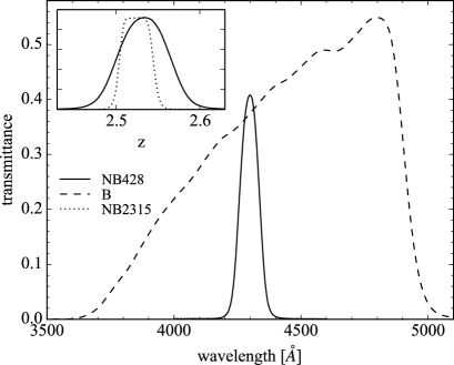
Figure 1: The black solid and the dashed curves indicate the filter response curves of NB428 and B-band on the Suprime-Cam, respectively. The upper left inset shows the filter response curves of NB428 on Suprime-Cam (solid curve) and NB2315 on MOIRCS (dotted curve) as a function of redshift for  Ly$\alpha$ and  H$\alpha$ lines, respectively.

The narrow-band (NB) filter, NB428, is installed on the Subaru Prime Focus Camera (Suprime-Cam; Miyazaki et al. 2002). It is a user filter belonging to R. Shimakawa (P.I. of this Paper) and is manufactured specifically for the purpose of searching for  Ly$\alpha$ emission and absorption lines at $z$=2.53$\pm$0.03. Its central wavelength and FWHM are 4297 Å and 84Å, respectively. It has a good spatial homogeneity of the central wavelength (less than $\pm 3$ Å) across the field of view. The NB428 filter makes a pair with our companion filter, NB2315, (belonging to Tadayuki Kodama; see Hayashi et al. 2012; Tadaki et al. 2013) which is installed on MOIRCS/Subaru. The NB2315 filter can sample  H$\alpha$ emitting star-forming galaxies at the same redshift of LAEs down to a  H$\alpha$ flux limit of 2.6$\times$10^-17 erg/s/cm². The filter response curves are shown in Figure 1.

LAEs at $z$=2.53 selected with the NB428 filter also have some great advantages. Those broad-band photometries of H_F160W and K_s do not include  H$\beta$$\lambda 4861$,  [Oiii]$\lambda\lambda 4959,5007$ or  H$\alpha$$\lambda 6563$ lines. This allows us to measure their accurate stellar masses and sizes from these broad-band data.  Ly$\alpha$$\lambda 1216$ line is also out of the response curve of the U-band of MegaCam on the Canada France Hawaii Telescope (CFHT). Moreover, all strong optical emission lines such as  H$\alpha$,  H$\beta$,  [Oiii], and  [Oii] lines including the  [Oiii]$\lambda 4363$ auroral line can be observed from the ground-based telescopes, which enable us to derive the robust measurements of gaseous metallicities based on the direct method (Izotov et al., 2006) by spectroscopic observations with future larger aperture telescopes.

2.1 Narrow-band imaging and data reduction

We performed a NB428 imaging observation with Suprime-Cam on UDS (Ultra Deep Survey; Lawrence et al. 2007; Foucaud et al. 2007) field on 2014 August 19, as a Subaru Service Program (S14B-198S; R. Shimakawa et al.). The wide field of view of Suprime-Cam (FoV=34’$\times$27’) covers the entire area of the UDS-CANDELS-WFC3/IR field (Grogin et al. 2011; Koekemoer et al. 2011; Fig. 2), where archive data are available including deep, high-resolution HST images. The NB observation was carried out in a standard manner with an individual exposure time of 1200 sec and two sets of five dithering points on a 1 arcmin radius circle. The total integration time amounted to 3.3 hrs, and the images were taken under a photometric sky condition with the seeing sizes of 0.62–0.86 arcsec, and the typical airmass of 1.2.

The obtained images were reduced by using a data reduction package for the Suprime-Cam, sdfred (ver.2; Yagi et al. 2002; Ouchi et al. 2004). This produces a well-reduced final image semi-automatically. The actual procedures consist of bias subtractions, flat fielding, distortion correction, PSF (point spread function) matching, sky subtraction, and image combining. More details of the pipeline are described in Ouchi et al. (2004). We also implement cosmic ray reduction using the algorithm of cosmic ray identification, L.A.Cosmic (van Dokkum, 2001). The final combined image has a seeing size of FWHM=0.85 arcsec, and the $5\sigma$ limiting magnitude of 26.63 in 1.5 arcsec diameter aperture. The zero point magnitude of 31.490 in 1200 sec is determined from a spectroscopic standard star, Feige 110, whose high-resolution spectrum was obtained by X-shooter on the Very Large Telescope (Moehler et al., 2014).

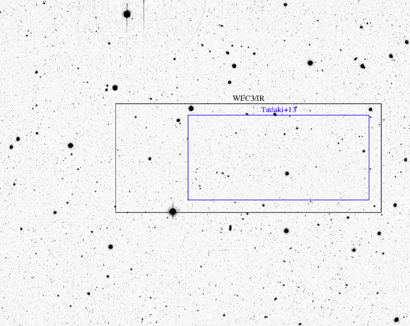
Figure 2: The reduced, full NB428 image (34’$\times$27’). This work concentrates on the overlapped area with the HST F160W image (WFC3/IR) which is marked with the black square (22’$\times$9’). We also incorporate the sample of  H$\alpha$ emitters at $z$=2.5 constructed within the narrower field shown by the blue square.

2.2 Colour magnitude diagram

We first identify narrow-band emitters by searching for objects that show flux excesses in the narrow-band (NB428) as compared to the broad-band (B). PSF size is matched to the NB428 image (FWHM=0.85 arcsec) and pixel scale is adjusted to mosaic image of B-band (0.268 arcsec/pixel) distributed by Cirasuolo et al. (2010). Hereafter we only use the data covering the UDS-CANDELS-WFC3/IR field (Fig. 2). The source identification is made using the astronomical software for source extraction called SExtractor (Bertin & Arnouts, 1996). Source detections are performed with the double-image mode of the SExtractor with detection parameters of detect_minarea=4, detect_thresh= 1.5, analysis_thresh= 2. We use a 1.5 arcsec diameter aperture both in NB428 and B-band to measure the object colours. Those 5$\sigma$ limiting magnitudes correspond to NB_5σ=26.55 and B_5σ=27.89 including the galactic extinction. The galactic extinctions of A_B=0.081 and A_NB428=0.082 mag are assumed based on the Fitzpatrick (1999) extinction law with R_V=3.1 and E(B$-$V) from Schlafly & Finkbeiner (2011), which is tailored to the specification in the 3D-HST catalogue (Skelton et al., 2014) that we use (§2.3). NB emitters are then selected by using a colour magnitude diagram of NB428 vs. B$-$NB (Fig. 3). We here apply a small correction to the NB magnitudes by $-0.1$ mag to remove an offset seen in the median B$-$NB colour of the bright galaxies (NB=24–25 mag). This offset would be mostly caused by a systematic zero-point offset due to the colour terms of individual galaxies. The amount of the colour terms are actually consistent with those predicted by the galaxies at the photometric redshift around 2.5 (see Appendix B). Because of this, this work does not consider a negligible colour term that originates from the small offset of the central wavelengths (170 Å) between NB428 and B-band. It actually has a strong benefit for searching LAEs having faint UV luminosities compared to similar studies for LAEs at slightly lower-$z$ which have used shallower U-band data (U_5σ=26.63 in the case of the UDS-CANDELS field). Then, we set the selection criteria: the observed equivalent width (EW_obs) is greater than 53 Å corresponding to 15 Å in the rest frame at $z=2.53$, B$-$NB$>$0.476 mag or $\sim 4\sigma$ scatter of NB$-$B for the luminous galaxies, the limiting magnitudes of $5\sigma$ ($2\sigma$) in NB (B) band, and the NB flux shows an excess of more than 3$\sigma$ compared to the B-band at 1.5 diameter aperture photometry, which is equivalent to a NB flux of 8.52$\times$10^-18 erg/s/cm² and a NB luminosity of 4.40$\times$10⁴¹ erg/s if they are located at $z=2.53$. We should note that B-band magnitude cut is not critical to our results and conclusions, since only two objects additionally selected as NB emitters without this threshold cannot pass all the selection criteria in this paper. In total, 123 galaxies satisfied these criteria, and they are represented by magenta circles in Fig. 3.

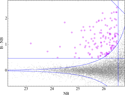
Figure 3: The colour-magnitude diagram of NB428 vs. B$-$NB428. The grey dots represent all the NB-detected galaxies in the UDS-WFC3 field. Stars with F160W$<$25 mag classified by Skelton et al. (2014) have been removed. The blue curves show the threshold of $\pm 3\sigma$ flux excess. The blue vertical and horizontal lines indicate the $5\sigma$ limiting magnitude and the criterion used for the observed equivalent width (EW_obs=53Å), respectively. The blue diagonal line indicates 2$\sigma$ limit of B-band. The purple open circles show the NB emitters that satisfy our selection criteria.

2.3 Catalogue matching

Since one motivation in this paper is to study physical properties of LAEs at $z=2.5$, multi-band photometry is required to derive their stellar masses, SFRs and so on. In particular, deep H_F160W-band photometry from the CANDELS (Grogin et al., 2011; Koekemoer et al., 2011) is critical to estimate robust stellar masses of low-mass LAEs at $z$=2.5. We perform a cross-matching of our NB-selected emitters to the sources in the 3D-HST catalogue (Skelton et al., 2014) which is constructed from the WFC3/HST images (F125W/F140W/F160W) taken by the CANDELS project (Grogin et al., 2011; Koekemoer et al., 2011) and the 3D-HST Treasury Survey (Brammer et al., 2012; Skelton et al., 2014). We employed a variety of photometric data in this catalogue covering a wide wavelength range from various imaging data; CFHT U-band (Almaini/Foucaud et al. in preparation), Subaru B,V,R,i,z-band (Furusawa et al., 2008), HST F606 and 814W (Koekemoer et al., 2011), UKIRT J,H,Ks (Lawrence et al. 2007; Almaini et al. in preparation), HST F140W (Brammer et al., 2012), F125 and 160W (Koekemoer et al., 2011). The catalogue includes the total fluxes correcting for the flux loss and also photometric zero-points in an empirical manner (see Skelton et al. 2014 for details). We first adjust the WCS information of the NB image to the combined image of WFC3/IR bands (F125W/F140W/F160W) made by 3D-HST based on the iraf task; ccmap and ccsetwcs. The coordinated WCS data of the NB image is well matched to those of WFC3 within less than 0.1 arcsec offset according to the positions of bright stars in each image. We then cross-matched the NB-selected sources to the 3D-HST catalogue, and select the galaxy closest to each NB emitter within a 0.4 arcsec radius. For 69 sources out of 123 NB emitters, we can find the counterparts. Most of the removed 54 objects should be very low-mass objects that are too faint even in the WFC3 image. Indeed, most of the catalogue-matched NB emitters are detected only at F125W and F160W bands in the NIR regime with more than a few sigma significance in 0.7 arcsec aperture diameter photometry. This work subsequently removes 11 very faint objects at F160W$>26.89$ that is 2$\sigma$ ($\sim 10\sigma$) limiting magnitude in 0.7 (0.35) arcsec aperture photometry (according to Skelton et al. 2014; Shibuya et al. 2014a). This value roughly corresponds to the stellar mass of $1\times 10^{8}$ solar mass at $z=2.53$.

Attentive considerations could be needed since spatial offsets of  Ly$\alpha$ peak (by a few arcsec at $z=2.2$) from the stellar continuum are often seen as shown by Shibuya et al. (2014a). Indeed, the peak locations of NB fluxes of some selected NB emitters seem to deviate from those of stellar continua seen in the WFC3 images. However, most of the NB emitters are as faint as $\sim$ 26 mag (less than 10$\sigma$ detections) in the NB magnitude. Thus it is hard to identify the spatial peaks in NB fluxes of those faint galaxies based only on the seeing-limited data. Furthermore, we also find that the separation angles between the peaks of NB fluxes and stellar continua of the NB emitters moderately correlate with their angular sizes, which means that flux peak locations of diffuse objects are not accurately measured. Because of this problem, we cannot resolve the spatial peaks of  Ly$\alpha$ emission robustly. This work employs the NB emitters, which were cross-matched to WFC3 source within 0.4 arcsec angular distance. This threshold is determined by the fact that 95% of the catalogue-matched galaxies are located within this criterion when we conduct the cross-matching by match criteria within 1.0 arcsec separation between NB sources and the 3D-HST sources.

Those processes were conducted using the Tool for OPerations on Catalogues And Tables (topcat; Taylor 2005, 2015).

2.4 Sample selection

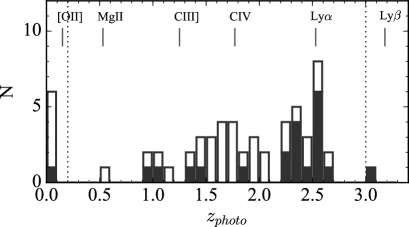
Figure 4: Photometric redshift distribution of the NB emitters by Momcheva et al. (2016). We employ the photometric redshift $z_{\mathrm{best}}$ in their catalogue. Filled and opened histograms present the NB emitters at F160W$\leq$25 and F160W$>$25 mag, respectively. This work simply remove the objects at photometric redshifts of $z_{\mathrm{best}}\leq 0.2$ or $3.0\leq z_{\mathrm{best}}$.

While the majority of them are likely to be LAEs at $z$=2.53$\pm$0.03, we need to remove some candidates, especially foreground  [Oii] line emitters at $z$=0.15 and background Lyman break galaxies and Ly$\beta$ emitters at $z>3$. We employed a photometric redshift catalogue by Momcheva et al. (2016), which is based on the combined technique of multi-band photometries and grism data by the 3D-HST Treasury Program. We simply excluded seven candidates of such contaminations showing photo-$z$ ($z_{\mathrm{best}}$) of $z_{\mathrm{best}}\leq 0.2$ or $3.0\leq z_{\mathrm{best}}$ in their catalogue. One should note that the redshift estimation by Momcheva et al. (2016) does not work well for our NB emitters because of their faintness at NIR bands, and thus photo-$z$ estimation should have larger uncertainties relative to their entire 3D-HST sample ($\sigma_{z}\sim 0.003\times(1+z)$ in $JH<24$). Actually photo-$z$ distribution of the NB emitters at F160W$>$25 mag systematically shifted toward $z<2$ as seen in the Figure 4. However, we believe that some of these would be LAEs at $z=2.5$ rather than foreground line emitters, because this trend has been reported by Shivaei et al. (2015) which show that estimation of photometric redshifts are systematically underestimated for faint at F160W and/or blue galaxies at $z$=2–2.6 like our LAE sample. On another front, it is highly likely that such  Mgii$\lambda 2800$,  Ciii]$\lambda 1909$, and  Civ$\lambda 1550$ emitters (at $z$=0.53, 1.25, and 1.77, respectively) are contained in LAE candidates especially for those at the bright end of the  Ly$\alpha$ luminosity function as noted by Sobral et al. (2016). Because of the lack of spec-$z$ confirmation of our LAE samples, we ignore these possible contaminations. However, we stress that our conclusions remain consistent even if we select the LAEs only within the photometric redshifts range of $z$=2.3–2.7. Moreover, this work mainly focuses on the physical properties of low-mass LAEs, and thus the contamination of bright foreground emitters may not be a big issue.

Finally, we carefully inspected multi band photometries of LAE candidates in order to check whether unrealistic objects still blend into our sample. We then find an object showing strange i-band excess ($\gtrsim 4\sigma$) relative to bluer and redder band photometries. It is highly likely that foreground  [Oii] emitters with $\gtrsim 50$ Å also have high EW of  H$\alpha$ line ($\lambda_{\mathrm{obs}}\sim 7560$ Å), which should cause i-band excess. Thus, this object considered a foreground  [Oii] emitter is also removed from the sample. Eventually, we obtained 50 LAE candidates at $z=2.5$. These selection processes are summarized in table 1.

Table 1: Selection proceeding of LAE candidates at $z=2.53$.

Selection criteria	removed	remained
NB emitters	—	123
Catalogue matching with 3D-HST ($<$0.4")	54	69
F160W/WFC3 magnitude cut ($\leq$26.89)	11	58
Photometric redshift cut ($0.2<z<3.0$)	7	51
i-band excess (contaminant  [Oii] emitters)	1	50

2.5 Final catalogue

The sample employed in this work consists of 50 LAEs at $z$=2.5. These are limited by the  Ly$\alpha$ luminosity ($>$4.40$\times$10⁴¹ erg/s), EW ($>$15 Å), and H_F160W band magnitude ($<$26.89 mag). Hereafter, we basically use their photometries from the 3D-HST catalogue (Skelton et al., 2014) except their  Ly$\alpha$ luminosities and equivalent widths (EWs), unless otherwise noted.

This work also collects HAE samples at the same redshift taken by the past narrow-band imaging survey of the UDS-CANDELS field with the MOIRCS on the Subaru telescope (Tadaki et al., 2013, 2014a). The data is limited to their observed  H$\alpha$ flux above $2.6\times 10^{-17}$ erg/s/cm², and more than EW_Hα of 40 Å in  H$\alpha$ emission at $z$=2.53. About half of them are spectroscopically confirmed by MOIRCS, KMOS, and ALMA. More details are described in Tadaki et al. (2013, 2014a); Tadaki et al. (2015), and forthcoming papers. We employ 37 out of 44 HAEs with B-band detections more than 2 sigma (28.88 mag) with 1.5 arcsec diameter photometry by the SExtractor. Two of those are also selected as LAEs by this observation. The B-band magnitude cut actually allows us to miss seven heavily obscured HAEs. However, this work neglects them in order to be consistent with the sample selection of LAEs, and also since we cannot constrain EWs of  Ly$\alpha$ of such dusty HAEs at all. After that, the HAE sample were cross-matched to the 3D-HST catalogue in the same manner as LAEs. Therefore, multi-band photometries of HAEs used in this work are a bit different from those reported by past studies.

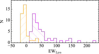
Figure 5: EW_Lyα distribution of LAEs (purple backslash) and HAEs (orange forward slash). Here, positive values show emissions and negative values mean absorptions.

Figure 5 represents EW_Lyα distributions of LAE and HAE samples. For HAEs without NB428 detections, we just insert 2 sigma upper limits. The stellar population model by Malhotra & Rhoads (2002) based on the Starburst99 (Leitherer et al., 1999) cannot explain extremely high EW${}_{\mathrm{Ly\alpha}}>240$ Å of  Ly$\alpha$ emission without the assumption of extreme IMF (much heavier IMF) (see also Charlot & Fall 1993; Schaerer 2002, 2003; Laursen et al. 2013). Fig. 5 indicates that our LAE selection does not contain such objects. On the other hand, we could not find strong  Ly$\alpha$ emission from the most of HAEs. Rather, we see a deficit in NB428 magnitude compared to B-band for a part of our HAE samples, which means that  Ly$\alpha$ line is in absorption rather than in emission for them. EW_Lyα distribution of HAEs seems consistent with that of Lyman-break galaxies at the similar redshift within the errors (Reddy et al., 2008). The details of such  Ly$\alpha$ absorbers and their possible origins are described in §3.3 and §4.3.

We then conducted SED-fitting based on the SED-fitting code fast distributed by Kriek et al. (2009). The SED fitting was carried out assuming a fixed redshift of $z$=2.53, the stellar population model of Bruzual & Charlot (2003), the Calzetti et al. (2000) attenuation curve, the Chabrier (2003) IMF and $Z$=0.008 metal abundance. Also, this allows truncated star formation history with constant star-formation in duration time of 10^6.5 to 10¹¹ yr, or delayed exponentially declining star-formation (SFR $\propto t\exp{(-t/\tau)}$) with log($\tau$/yr)=6.5–11. Then, star-formation history that gives better least chi square value is assigned. Here, log(age/yr) between 6 and 9 are given. Band photometries and errors of U,B,V,R,i,z,J,H,K,F606,814,125,140,160W from the 3D-HST catalogue are used, where  Ly$\alpha$ and  H$\alpha$ flux contaminations to B band and K band for LAEs and HAEs are corrected, respectively. $1\sigma$ errors of obtained values such as stellar mass are measured by 500 Monte Carlo simulations attached with the fast code. As a result, the median reduced chi-squares of the fitting results show 1.18 and 1.83 in HAE and LAE samples, respectively.

Figure 6: Examples of SED-fitting for LAEs (upper panel) and HAEs (lower panel). Purple and orange circles indicate observed broad-band flux densities, and large red circles are flux densities of NB428. Black lines represent the inferred spectra by SED-fitting.

Fig. 6 represents examples of the SED-fitting for LAEs and HAEs at $z=2.5$. We can see strong excess and deficit of NB flux density in LAE and HAE, respectively. As compared to the HAE sample, LAEs tend to be faint at all broad-bands, and especially in the NIR regime F160W photometry is quite essential to determine their stellar masses. It should be noted again that emission line contaminations to broad-band photometries are negligible for our sample because F160W band does not include any strong emission line, and the fitting results remain consistent even if we apply restricted broad-band datasets which do not contain strong emission lines ( [Oii], H$\beta$  [Oiii], H$\alpha$) to the SED-fitting. We also confirmed that measured stellar masses of all line emitters remain consistent regardless of assumption of star-formation history.

In addition to the measurements of physical properties by the SED-fitting, we also estimate dust attenuation from the UV slope $\beta$ ($f_{\lambda}\propto\lambda^{\beta}$) in accordance with the Meurer et al. (1999); Calzetti et al. (2000) relation. The UV slopes of all the emitters are calculated by error-weighted least chi square fitting based on V,R,i,F606W band photometries corresponding to $\lambda$=1500–2500 Å in the rest frame. We then estimate their 1 sigma errors by 1000 Monte Carlo iterations. Recent studies tend to prefer to estimate the stellar dust extinction from the UV slope since the dust reddening inferred from the whole SED-fitting would inevitably depend on the stellar mass estimates (Shivaei et al., 2015). While the measured values of the UV slope for most of the LAEs comfortably fall into the reasonable range inferred from the Meurer et al. (1999) relation within the margins of errors, there are several LAEs which has very blue UV slopes ($\beta<-2.3$) deviating from the relation (Table 2). Such an extremely blue UV slope would require a large contribution of stellar populations of instantaneous starburst of the age $\lesssim 10^{7}$ yr (Leitherer & Heckman, 1995; Calzetti, 2001) to the UV spectrum. In this paper, we simply apply "zero" extinction for them. On the other hand, SED-inferred extinction could be helpful since it may resolve varieties of stellar populations in such young LAEs. Therefore, we also check the results if we apply the SED-inferred extinctions, and those can be found in Appendix A.

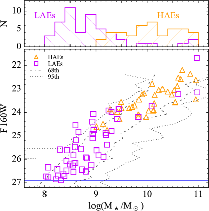
Figure 7: The upper histogram shows log stellar mass distributions of LAEs (purple backslash) and HAEs (orange forward slash), and the lower panel presents log stellar mass versus F160W magnitude. The squares and the triangles are LAEs and HAE, respectively. The horizontal line indicates 2$\sigma$ magnitude cut of F160W=26.89. Dash-dot and dotted lines indicate the region enclosing 68% and 95% of photo-$z$ selected galaxies at $z$=2.3–2.8 for a given F160W, based on the 3D-HST catalogue (Skelton et al., 2014). Our LAE sample is relatively complete above the stellar mass of $\sim$10^8.5 M_⊙, while even lower mass LAEs should be biased toward more active (bluer) star-forming galaxies.

Figure 7 shows measured stellar mass distributions of LAEs and HAEs. LAEs tend to have lower stellar masses relative to  H$\alpha$-flux limited sample. Although our sample size is not sufficient, our LAE sample in the target area would be relatively complete above the stellar mass of log(M_⋆/M_⊙)$\sim$8.5 if the number of LAEs increase in smaller stellar masses. In the meantime, the lower panel in Fig. 7 shows F160W magnitudes as a function of log stellar mass of our all emitter sample. The figure also shows those enclosing 68% and 95% of galaxies at the photometric redshift of 2.3–2.8 for a given F160W, which is taken from the Skelton et al. (2014) catalogue. This suggests that the magnitude limit of F160W$<$26.89 can cover down to the stellar mass of $\sim$10^8.5 M_⊙. On the other hand, it also denotes that our selection should be biased toward galaxies with high mass-to-light ratios (i.e. more actively star-forming and bluer galaxies) in even lower mass regime $\lesssim$10^8.5 M_⊙. Similarly, we would have only active star-forming systems for the HAE sample below the stellar mass $\sim$10¹⁰ M_⊙.

The position of NB flux peaks and cross-matched ID number in the 3D-HST catalogue (Skelton et al., 2014) and photometric redshifts by Momcheva et al. (2016) for all LAEs can be found in Table 2. This also describes the values and 1 sigma errors of those  Ly$\alpha$ luminosities,  Ly$\alpha$ equivalent widths in the rest frame, UV slopes, stellar masses, dust-corrected SFRs based on E(B$-$V) from UV slope and SED-fitting, and effective radii from van der Wel et al. (2012).

Table 2: Final LAE catalogue at $z=2.5$. The first column shows identification number of LAEs. The second and fifth columns indicate identification number in the 3D-HST UDS catalogue (Skelton et al., 2014) and photometric redshifts ($z_{\mathrm{best}}$) and those 68th percentiles from Momcheva et al. (2016), based on the 3D-HST Treasury Survey. The second and third show peak position of NB flux. The sixth to ninth represent values and 1 sigma errors of  Ly$\alpha$ luminosity (E41 erg/s), EW of  Ly$\alpha$ line emission in the rest frame (Å), UV slope $\beta$, log stellar mass. The 10th and the 11th are SFRs from UV luminosity (M_⊙/yr) where those dust extinctions are corrected, following UV slope and SED-fitting, respectively. The 12th are effective radii derived from galfit distributed by van der Wel et al. 2012 (flags indicate the fitting results defined by their paper; $s$=suspicious, $b$=bad). Full table is available as online material.

1ID	2IDHST	3R.A.NB	4Dec.NB	5$z_{\mathrm{best}}$	6LE41	7EW	8$\beta$	9logM⋆	10SFR${}_{\mathrm{UV_{\beta}}}$	11SFR${}_{\mathrm{UV_{sed}}}$	12Re
1	5917	34.54872	$-$5.25659	1.71	3.4$\pm$1.4	23$\pm$5	$-$2.71$\pm$0.39	8.73${}_{-1.02}^{+0.18}$	1.0${}_{-0.1}^{+4.9}$	1.0${}_{-0.1}^{+1.2}$	b0.38$\pm$0.42
7	10425	34.56473	$-$5.24084	2.58	12.7$\pm$2.4	21$\pm$4	$-$1.74$\pm$0.03	9.20${}_{-0.80}^{+0.17}$	5.3${}_{-3.3}^{+17.4}$	6.8${}_{-4.8}^{+6.3}$	1.12$\pm$0.36
9	14560	34.55527	$-$5.22678	2.04	13.6$\pm$2.2	39$\pm$5	$-$2.77$\pm$0.16	8.59${}_{-0.58}^{+0.50}$	2.4${}_{-0.2}^{+10.8}$	2.4${}_{-0.2}^{+4.6}$	1.52$\pm$0.85
12	18325	34.56935	$-$5.21441	1.42	20.8$\pm$1.5	140$\pm$24	$-$2.85$\pm$0.35	8.60${}_{-0.80}^{+0.26}$	0.8${}_{-0.2}^{+4.0}$	0.8${}_{-0.2}^{+1.5}$	0.75$\pm$0.54
15	18990	34.55072	$-$5.21225	1.11	9.6$\pm$1.7	21$\pm$4	$-$1.54$\pm$0.25	8.30${}_{-0.22}^{+0.68}$	7.9${}_{-5.9}^{+26.6}$	7.0${}_{-5.0}^{+5.7}$	2.35$\pm$1.60
22	37097	34.58892	$-$5.15123	2.23	46.0$\pm$1.9	15$\pm$0	$-$2.40$\pm$0.21	9.45${}_{-0.06}^{+0.22}$	8.3${}_{-0.1}^{+37.6}$	8.3${}_{-0.1}^{+5.9}$	1.69$\pm$0.12
27	34511	34.51098	$-$5.16014	1.56	5.6$\pm$1.4	41$\pm$9	$-$2.14$\pm$0.38	8.22${}_{-1.09}^{+0.34}$	0.6${}_{-0.2}^{+2.9}$	0.5${}_{-0.1}^{+0.6}$	b0.62$\pm$0.84
28	28289	34.56316	$-$5.18097	2.41	48.6$\pm$2.9	16$\pm$1	$-$2.28$\pm$0.23	8.60${}_{-0.05}^{+0.68}$	5.0${}_{-0.1}^{+22.8}$	15.7${}_{-10.9}^{+5.4}$	1.28$\pm$0.16
29	32164	34.50610	$-$5.16808	2.54	18.4$\pm$1.8	20$\pm$2	$-$1.91$\pm$0.20	8.66${}_{-0.00}^{+0.08}$	6.8${}_{-3.1}^{+26.6}$	18.8${}_{-2.6}^{+4.4}$	0.61$\pm$0.19
30	30895	34.50703	$-$5.17256	2.33	49.0$\pm$1.5	38$\pm$1	$-$2.14$\pm$0.22	9.42${}_{-0.16}^{+0.16}$	6.3${}_{-1.0}^{+27.6}$	10.7${}_{-5.4}^{+3.2}$	1.43$\pm$0.14
m31	30133	34.54215	$-$5.17551	1.84	136$\pm$1.4	48$\pm$0	$-$1.58$\pm$0.41	10.97${}_{-0.31}^{+0.19}$	52.0${}_{-36.5}^{+193}$	628${}_{-612}^{+825}$	1.11$\pm$0.05
35	3182	34.48001	$-$5.26605	2.51	11.7$\pm$1.3	68$\pm$13	$-$0.41$\pm$0.09	10.61${}_{-0.08}^{+0.07}$	26.2${}_{-24.9}^{+24.9}$	22.5${}_{-21.7}^{+24.5}$	1.23$\pm$0.06
36	4309	34.44040	$-$5.26320	2.51	7.7$\pm$1.5	77$\pm$24	$-$0.36$\pm$0.26	10.98${}_{-0.22}^{+0.10}$	30.9${}_{-30.0}^{+36.1}$	24.1${}_{-23.3}^{+43.5}$	2.97$\pm$0.13
41	10396	34.43763	$-$5.24091	1.90	10.9$\pm$1.6	173$\pm$33	$-$2.18$\pm$0.50	8.81${}_{-0.38}^{+0.17}$	0.4${}_{-0.1}^{+1.9}$	0.4${}_{-0.1}^{+0.6}$	1.10$\pm$0.73
47	20895	34.47444	$-$5.20549	2.43	5.5$\pm$1.6	30$\pm$7	$-$1.74$\pm$0.03	8.50${}_{-0.28}^{+0.42}$	1.6${}_{-1.0}^{+5.2}$	0.6${}_{-0.1}^{+1.7}$	b1.35$\pm$0.62
56	27668	34.47025	$-$5.18285	0.56	6.2$\pm$1.4	34$\pm$8	$-$2.78$\pm$0.31	8.07${}_{-0.60}^{+0.40}$	1.5${}_{-0.1}^{+7.3}$	1.9${}_{-0.5}^{+3.7}$	2.00$\pm$1.26
57	27420	34.42780	$-$5.18368	2.40	11.7$\pm$1.6	51$\pm$11	$-$2.00$\pm$0.40	9.15${}_{-0.93}^{+0.16}$	1.8${}_{-0.8}^{+8.1}$	3.0${}_{-1.9}^{+4.9}$	b1.88$\pm$1.12
58	26371	34.48166	$-$5.18751	2.54	23.6$\pm$2.4	19$\pm$3	$-$1.75$\pm$0.27	8.61${}_{-0.13}^{+0.54}$	5.2${}_{-3.1}^{+19.5}$	16.9${}_{-9.8}^{+13.6}$	b1.82$\pm$0.29
60	24704	34.46305	$-$5.19313	2.66	22.6$\pm$1.4	15$\pm$1	$-$1.77$\pm$0.31	8.95${}_{-0.00}^{+0.65}$	11.1${}_{-6.5}^{+42.9}$	47.2${}_{-42.6}^{+13.1}$	0.87$\pm$0.11
61	24397	34.47254	$-$5.19386	2.64	9.8$\pm$1.9	223$\pm$90	$-$2.39$\pm$0.33	8.39${}_{-0.26}^{+0.38}$	0.2${}_{-0.0}^{+1.0}$	0.2${}_{-0.0}^{+1.2}$	b0.98$\pm$0.63
63	5744	34.40507	$-$5.25718	2.23	24.4$\pm$2.5	22$\pm$2	$-$2.09$\pm$0.25	8.94${}_{-0.30}^{+0.16}$	3.6${}_{-0.9}^{+15.6}$	5.5${}_{-2.8}^{+3.2}$	0.78$\pm$0.23
64	11017	34.32240	$-$5.23897	2.20	21.2$\pm$1.7	50$\pm$4	$-$2.26$\pm$0.36	8.43${}_{-0.58}^{+0.36}$	1.3${}_{-0.1}^{+6.4}$	2.7${}_{-1.4}^{+2.0}$	b1.06$\pm$0.79
67	12523	34.33171	$-$5.23398	2.51	25.1$\pm$1.6	31$\pm$3	$-$2.26$\pm$0.22	8.44${}_{-0.18}^{+0.43}$	2.0${}_{-0.1}^{+9.1}$	15.8${}_{-13.9}^{+19.0}$	b0.87$\pm$0.28
73	18238	34.32620	$-$5.21464	1.89	2.8$\pm$1.3	41$\pm$12	$-$1.75$\pm$0.56	8.55${}_{-0.69}^{+0.41}$	3.9${}_{-2.5}^{+16.6}$	3.1${}_{-1.8}^{+6.5}$	b142$\pm$153
74	18921	34.34030	$-$5.21269	2.00	5.7$\pm$1.4	24$\pm$3	$-$2.36$\pm$0.31	9.22${}_{-0.35}^{+0.06}$	1.9${}_{-0.1}^{+8.8}$	1.9${}_{-0.1}^{+1.4}$	b2.59$\pm$0.66
76	39205	34.34621	$-$5.14343	2.00	41.4$\pm$1.4	97$\pm$7	$-$2.21$\pm$0.19	8.56${}_{-0.58}^{+0.20}$	1.5${}_{-0.1}^{+6.7}$	4.7${}_{-3.3}^{+5.1}$	0.67$\pm$0.19
78	37204	34.37653	$-$5.15058	2.37	15.9$\pm$1.7	51$\pm$7	$-$2.11$\pm$0.18	9.01${}_{-0.73}^{+0.24}$	1.3${}_{-0.3}^{+5.4}$	5.2${}_{-4.2}^{+5.8}$	1.16$\pm$0.39
79	22942	34.39716	$-$5.19887	2.56	17.8$\pm$1.3	38$\pm$3	$-$1.88$\pm$0.28	8.94${}_{-0.33}^{+0.32}$	4.9${}_{-2.4}^{+19.6}$	3.2${}_{-0.8}^{+6.4}$	1.08$\pm$0.24
84	29768	34.31855	$-$5.17587	1.41	14.3$\pm$1.6	112$\pm$20	$-$2.86$\pm$0.40	8.37${}_{-0.43}^{+0.19}$	0.6${}_{-0.1}^{+3.0}$	0.6${}_{-0.1}^{+0.4}$	b1.11$\pm$1.03
h87	27615	34.36791	$-$5.18348	2.39	83.7$\pm$2.3	27$\pm$0	$-$2.26$\pm$0.25	9.31${}_{-0.15}^{+0.14}$	7.2${}_{-0.1}^{+33.3}$	9.1${}_{-2.0}^{+6.3}$	s2.59$\pm$0.14
90	24644	34.34509	$-$5.19317	1.71	20.0$\pm$1.3	139$\pm$26	$-$3.17$\pm$0.23	8.32${}_{-0.54}^{+0.21}$	0.5${}_{-0.1}^{+2.3}$	0.5${}_{-0.1}^{+0.5}$	b1.51$\pm$1.46
91	24422	34.38580	$-$5.19380	1.68	27.7$\pm$2.0	56$\pm$5	$-$2.47$\pm$0.20	8.58${}_{-0.91}^{+0.26}$	1.6${}_{-0.1}^{+7.3}$	1.6${}_{-0.1}^{+1.5}$	b2.24$\pm$1.31
92	22925	34.34627	$-$5.19876	1.53	12.8$\pm$1.8	41$\pm$9	$-$1.95$\pm$0.53	8.25${}_{-0.61}^{+0.36}$	2.1${}_{-1.0}^{+9.6}$	1.2${}_{-0.2}^{+1.1}$	b0.48$\pm$0.42
93	2452	34.22792	$-$5.26813	1.72	5.4$\pm$0.9	48$\pm$15	$-$2.74$\pm$0.42	8.56${}_{-0.77}^{+0.38}$	0.7${}_{-0.1}^{+3.5}$	0.7${}_{-0.1}^{+1.7}$	0.51$\pm$0.42
94	2967	34.23742	$-$5.26633	1.91	7.8$\pm$1.0	36$\pm$10	$-$1.87$\pm$0.22	8.91${}_{-0.93}^{+0.15}$	1.1${}_{-0.7}^{+4.3}$	1.4${}_{-1.0}^{+2.0}$	0.60$\pm$0.40
95	3013	34.22358	$-$5.26614	1.00	6.8$\pm$1.7	21$\pm$4	$-$0.60$\pm$0.38	8.71${}_{-0.29}^{+0.34}$	24.1${}_{-23.0}^{+43.9}$	46.1${}_{-45.1}^{+28.1}$	1.21$\pm$0.30
100	8055	34.28063	$-$5.24924	2.39	15.7$\pm$2.2	24$\pm$2	$-$2.59$\pm$0.12	8.96${}_{-0.09}^{+0.27}$	2.9${}_{-0.1}^{+12.6}$	2.9${}_{-0.1}^{+1.7}$	4.85$\pm$1.48
101	8542	34.29174	$-$5.24732	1.74	17.5$\pm$2.1	43$\pm$8	$-$1.82$\pm$0.44	8.43${}_{-0.61}^{+0.17}$	2.1${}_{-1.2}^{+9.0}$	20.1${}_{-19.2}^{+9.9}$	0.36$\pm$0.19
102	9191	34.22307	$-$5.24571	1.40	4.3$\pm$1.6	17$\pm$3	$-$0.85$\pm$0.24	10.09${}_{-0.00}^{+0.27}$	22.9${}_{-21.3}^{+46.9}$	2.2${}_{-0.5}^{+8.0}$	6.24$\pm$0.54
108	12330	34.30823	$-$5.23463	1.67	28.2$\pm$2.3	71$\pm$6	$-$2.28$\pm$0.41	8.83${}_{-0.17}^{+0.09}$	1.3${}_{-0.1}^{+6.4}$	1.3${}_{-0.1}^{+0.3}$	0.51$\pm$0.24
110	18016	34.29846	$-$5.21541	1.39	12.1$\pm$1.9	24$\pm$4	$-$2.88$\pm$0.05	9.19${}_{-0.35}^{+0.15}$	1.2${}_{-0.1}^{+5.2}$	4.9${}_{-3.8}^{+17.5}$	0.71$\pm$0.13
111	18221	34.27096	$-$5.21479	1.39	7.3$\pm$1.1	87$\pm$23	$-$2.15$\pm$0.38	8.26${}_{-0.60}^{+0.34}$	0.5${}_{-0.2}^{+2.5}$	0.5${}_{-0.1}^{+1.4}$	b0.80$\pm$0.45
112	18947	34.22298	$-$5.21232	1.62	7.3$\pm$1.4	23$\pm$4	$-$2.54$\pm$0.33	8.81${}_{-0.37}^{+0.29}$	1.1${}_{-0.1}^{+5.3}$	2.2${}_{-1.2}^{+3.4}$	1.13$\pm$0.37
d114	29191	34.25741	$-$5.17772	1.04	11.0$\pm$1.4	148$\pm$53	$-$2.46$\pm$0.33	9.05${}_{-0.48}^{+0.23}$	0.2${}_{-0.2}^{+1.1}$	0.2${}_{-0.2}^{+1.3}$	b0.98$\pm$0.69
117	34684	34.24193	$-$5.15978	2.50	34.2$\pm$1.9	23$\pm$1	$-$1.70$\pm$0.18	9.25${}_{-0.00}^{+0.07}$	11.7${}_{-7.4}^{+40.8}$	69.1${}_{-2.0}^{+16.0}$	1.10$\pm$0.09
h118	33079	34.24434	$-$5.16520	2.40	29.0$\pm$1.4	36$\pm$2	$-$1.82$\pm$0.14	9.83${}_{-0.02}^{+0.07}$	5.9${}_{-3.2}^{+21.6}$	4.4${}_{-0.5}^{+3.6}$	0.42$\pm$0.06
119	32712	34.23558	$-$5.16694	1.04	16.3$\pm$2.9	36$\pm$5	$-$0.67$\pm$0.47	8.93${}_{-0.42}^{+0.47}$	41.6${}_{-39.5}^{+88.0}$	14.4${}_{-12.4}^{+28.3}$	5.82$\pm$1.34
121	28511	34.24313	$-$5.18004	1.70	13.0$\pm$1.8	54$\pm$10	$-$1.83$\pm$0.41	8.03${}_{-0.58}^{+0.48}$	1.9${}_{-1.1}^{+7.9}$	0.9${}_{-0.1}^{+2.2}$	b0.14$\pm$0.19
122	27412	34.26027	$-$5.18367	1.51	13.0$\pm$1.4	95$\pm$23	$-$1.50$\pm$0.24	8.07${}_{-0.50}^{+0.59}$	1.7${}_{-1.4}^{+5.6}$	1.8${}_{-1.4}^{+4.6}$	b1.85$\pm$1.95
123	24058	34.27530	$-$5.19516	2.23	14.5$\pm$1.9	21$\pm$3	$-$0.42$\pm$0.29	9.31${}_{-0.32}^{+0.11}$	54.7${}_{-52.9}^{+72.8}$	2.4${}_{-0.6}^{+2.4}$	b2.83$\pm$0.36
h  H$\alpha$ emitters at $z$=2.5 selected by Tadaki et al. (2013, 2014a).
m MIPS 24$\micron$m sources found by SpUDS (Dunlop et al., 2007) overlap those objects within 3 arcsec radius.
x All LAEs have no X-ray source detected by Subaru/XMM-Newton Deep Survey (Ueda et al., 2008) within 3 arcsec radius.
d affected by diffraction spikes in HST images.

3 Results

3.1 Main sequence

We now study star-forming activities of the LAEs as well as those of HAEs at $z=2.53$. We employ UV luminosities measured from V-band magnitudes, which correspond to the UV flux densities at $\sim$1600 Å in the rest frame. The deep  Ly$\alpha$ data and multi-band datasets allow us to reach and investigate the low-mass end of the main sequence at $z$=2.5. As mentioned in the previous section, LAEs below the stellar mass of log(M_⋆/M_⊙)$=$8.5 will be weighted toward more active star-forming systems.

Since  Ly$\alpha$ emission line is located at UV wavelength range unlike rest-frame optical emission lines like  H$\alpha$, the selection effect is critical when one studies star-forming activities in LAEs. This is especially true for narrow-band selected LAEs, which ought to be biased to LAEs with high EWs. In the case of  Ly$\alpha$ emission line, EW_Lyα is always lower than $\sim$240Å according to the stellar population model unless we take into account the contributions from Pop-III type objects, accreting binary stars, and/or rapidly rotating massive stars (Schaerer, 2003; Malhotra & Rhoads, 2002; Kashikawa et al., 2012; Trainor et al., 2016). Thus the shallow spectroscopic survey of LAEs is likely to be biased toward LAEs with luminous UV flux densities ($\gtrsim L_{\mathrm{Ly\alpha}}$/240 erg s^-1Å^-1) as well. Assuming the typical UV slope of $\beta=-2.2$ seen in our low-mass LAEs ($<$10¹⁰ M_⊙), the depths of our narrow-band and B-band data (NB_5σ=26.55 and B_5σ=27.89, respectively) can capture LAEs with EW${}_{\mathrm{Ly\alpha}}\geq 15$, 20, and 50 Å down to SFRs of 0.8, 0.5, and 0.3 M_⊙/yr, respectively. Therefore, our data are able to reach typical star-forming activities of galaxies with the stellar masses down to $\sim 10^{8}$ M_⊙ according to the extrapolated main sequence of massive star-forming galaxies at similar redshfits (Skelton et al., 2014; Shivaei et al., 2015; Tomczak et al., 2016). This is a great advancement compared to other similar studies such as Vargas et al. (2014); Hagen et al. (2014, 2016); Oteo et al. (2015) which are limited towards LAEs with higher SFRs due to larger line luminosity limits.

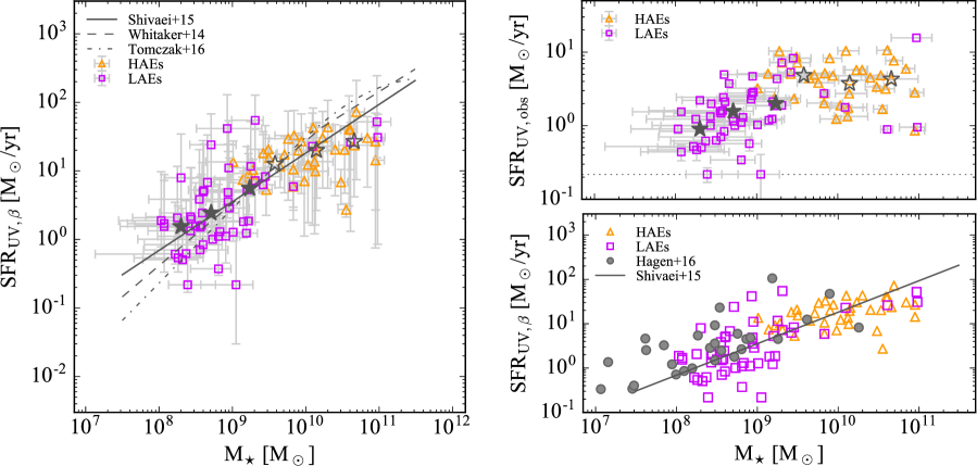
Figure 8: (a) The left panel shows the stellar mass versus dust-corrected SFR, SFR$\mathrm{UV,\beta}$. Extinction correction is based on UV slope. (b) The upper right panel presents dust-uncorrected SFR, SFR_UV,obs, and (c) the bottom right panel shows the same as (a), but the result by Hagen et al. (2016) are also plotted for comparison (grey filled circles). Orange triangles and purple squares represent HAEs and LAEs at $z=2.5$ (this work). The observed UV luminosities are measured from V-band, and the $2\sigma$ limiting magnitude in V-band (V=28.19) is shown by the dotted horizontal line in the panel (c). The black filled stars in panels (a) and (b) indicate the median SFRs of the LAEs in the stellar mass bins in logarithmic scale of $<$8.5, 8.5–9.0, and 9.0–10.0, while the open stars present the median SFRs of HAEs at the log stellar masses of $<$10.0, 10.0–10.5, and $>$10.5. In the panel (a), dashed, dot-dash, and solid lines respectively show the main sequences of the star-forming galaxies at $z$=2.0–2.5 reported by Whitaker et al. (2014), the one at $z$=2.5 obtained by the prescription in Tomczak et al. (2016), and the one at $z$=2.0–2.6 by Shivaei et al. (2015). The SFRs are all obtained based on UV+IR luminosities in Whitaker et al. (2014); Tomczak et al. (2016), and the same manner as our measurement in Shivaei et al. (2015), respectively. Since the main sequences for comparison are derived only for massive galaxies above $1\times 10^{9}$ or $1\times 10^{10}$ M_⊙ at $z\sim 2.5$, we just linearly extrapolate the relations to the lower mass regime. The measurements of SFRs (and dust correction) using other methods are also presented in the Appendix.

Figure 8b presents stellar masses versus dust-uncorrected SFRs of the LAEs and HAEs. We measure the SFRs based on the Kennicutt (1998) conversion assuming the Chabrier (2003) IMF. The $2\sigma$ limiting magnitude at V-band is 28.19 mag which corresponds to the SFR limit of 0.2 M_⊙/yr. The $2\sigma$ flux densities are assumed for two emitters that are fainter than this threshold. The median values are calculated in each mass bin corresponding to log stellar mass $<$8.5, 8.5–9.0, and 9.0–10.0 for LAEs, and log stellar mass $<$10.0, 10.0–10.5, and $>$10.5 for HAEs, respectively. Since more massive galaxies (HAEs) tend to be dustier and/or beginning to be quenched, the slope of the mass vs. UV luminosity relation turns over at the massive end roughly above $1\times 10^{10}$ M_⊙. On the other hand, most of the LAEs contain only a small amount of dust and tend to be less massive. Therefore, they show a positive correlation between stellar masses and observed UV luminosities even without a dust correction.

We then estimate the dust-corrected SFRs of our sample and make an improved mass–SFR relation (star-forming main sequence) (Daddi et al., 2007; Elbaz et al., 2007; Noeske et al., 2007), which is compared to earlier but recent measurements in the literature (Speagle et al., 2014; Whitaker et al., 2014; Shivaei et al., 2015; Tomczak et al., 2016). The extinction levels are obtained based on the UV slope (Fig. 8a) or the SED-fitting (Appendix A) as mentioned in §2.5. The SED-inferred SFRs are also shown in the Appendix. Before a comparison is made, several remarks should be noted. The main sequences reported by (Whitaker et al., 2014; Tomczak et al., 2016) are obtained by UV+IR luminosities from the stacked data of photo-$z$ selected galaxies. On the other hand, Shivaei et al. (2015) reported the main sequence of spectroscopically confirmed galaxies at $z=$2–2.6 selected by F160W-band magnitude limit ($<25$ mag), and they have studied the main sequence with different varieties of SFR measurements. In Fig. 8a,c, the main sequence from Shivaei et al. (2015) is based on SFR from UV with dust correction by UV slope, which is the same way as our estimation here. The choice of SFR calibration and this impact on measurements of the main sequence is beyond the scope of this paper. However, it is important to check and discuss this bias. Thus this paper also shows the same diagrams from different SFR measurements in the Appendix A.

Although our LAEs are widely spread in stellar mass, the median values follow neatly along the linearly extrapolated lines of the main sequences of Whitaker et al. (2014); Shivaei et al. (2015); Tomczak et al. (2016) as shown in Fig. 8a. The measured SFRs and stellar masses of individual LAEs are given in Table 2, and the median values plotted in the Fig 8 are also listed in Table 3. Two HAEs classified also as LAEs just overlap each other in the figures. It should be noted that this paper has not used seven heavily obscured HAEs missing B-band detections to be consistent with the LAE selection (see §2.5). This selection effect underestimates the median values of HAEs at the massive end ($>10^{10.5}$), which include five out of those in the Fig. 8.

In Fig. 8c, the distribution of our LAE sample on the mass–SFR diagram is clearly different from that of LAEs at $z$=1.9–2.3 explored by Hagen et al. (2016). Such inconsistency is likely to be caused by the shallower data in Hagen et al. (2016). However, we should notify that Hagen et al. (2016) have confirmed the same mass–SFR distribution between LAEs and their ‘control’ non-LAE sample in their paper. In that sense, our result is consistent with the report by Hagen et al. (2016), and indeed the mass–SFR distribution in their LAEs do not deviate from those of relatively active star-forming LAEs in our sample.

Our data now confirm that the low-mass LAEs are located along the expected, extrapolated line of the main sequence of normal massive star-forming galaxies towards lower stellar masses. However, it should be noted that we do not know whether the LAEs are the representative populations of the low-mass systems at this redshift because only $\sim 10\%$ of star-forming galaxies would be selected as LAEs (Hayes et al., 2010; Cassata et al., 2015; Matthee et al., 2016; Hathi et al., 2016; Sobral et al., 2016). Moreover, we do not have a comparison sample (i.e. non- Ly$\alpha$-emitting galaxies) at the mass regime below $1\times 10^{9}$ M_⊙.

On the other hand, such a similarity of star-forming activities between LAEs and normal star-forming galaxies may not apply to more massive LAEs. Four LAEs with the stellar mass of $>10^{9.5}$ solar mass tend to be located below the main sequence, which is notable in SFR_UV,sed and SFR_SED (see Appendix). Such less-active LAEs are also discovered by Taniguchi et al. (2015). We discuss these LAEs in §4.2.

3.2 Mass-size relation

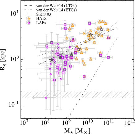
Figure 9: Stellar masses versus effective radii R_e of LAEs and HAEs at $z=2.5$. The symbols are the same as in Fig. 8, but the objects whose effective radii are not fitted well and marked as ‘bad fit’ in the catalogue of van der Wel et al. (2012), are shown by the cross marks. The hatched region corresponds to the size of bright stars ($\pm 1\sigma$). The Dashed and dotted lines indicate the mass-size relations of late-type and early-type galaxies at $z$=2.0–2.5 reported by van der Wel et al. (2014), respectively. Dotted curve shows the local mass–size relation of late-type galaxies (Shen et al., 2003).

Typical LAEs follow the extrapolated line of the main sequence of massive star-forming galaxies as presented in the previous section. How about their stellar angular sizes? In this section, we explore the positions of the LAEs on the mass–size diagram. We use the effective radii on the semi-major axis which are measured from the HST F160W image and listed in the catalogue of van der Wel et al. (2012, 2014). They use the software, galfit (Peng et al., 2010) combined with galapagos (Barden et al., 2012) in order to measure the precise background levels. Details of the fitting procedure and associated error estimation can be found in their paper. Since their catalogue uses the same identification numbers as those in the 3D-HST catalogue (Skelton et al., 2014), we were easily able to obtain the stellar sizes for all the LAEs, by cross-matching the catalogues.

The result is shown in Figure 9. Because of the faintness of the sources, no reliable fitting results can be obtained for 20 out of all the 50 LAEs in the F160W image, and they are marked as ‘bad fit’ or ‘suspicious fit’ in the van der Wel et al. (2012) catalogue. It is quite hard to measure the sizes of the low-mass LAEs below $1\times 10^{9}$ M_⊙, in particular for diffuse (lower surface brightness) LAEs. Even if the fits are reasonably good, LAEs tend to be faint in F160W images, and their morphologies are largely unresolved. In this section, we only employ the effective radii in their catalogue. However, the size measurements of faint objects at F160W/IR image are uncertain (see also Shibuya et al. 2015), and the results should be seen with this caution in mind.

Although the size measurements of the LAEs tend to have large error-bars compared to the HAEs at the same redshift, the LAEs seem to lie on the area where the mass–size relation of star-forming galaxies at $z$=2–2.5 by van der Wel et al. (2014) is extrapolated to the lower mass regime. We do not find any statistical difference in their angular sizes with respect to the HAEs along the mass-size relation. We also check and confirm that the distribution of our LAE sample on the mass–size diagram agrees well with that of LAEs at $z\sim 2$ by Hagen et al. (2016), which also reports a consistent mass–size distribution between non-LAEs and LAEs at the same stellar mass range. We also confirm that the size of our LAEs are consistent with those of LAEs at $z=2.1$ and 3.1 by Bond et al. (2012), based on the measurements with the SExtractor (Skelton et al., 2014).

Our result suggests that the stellar sizes of low-mass LAEs are not biased, and they are seen as just normal low-mass star-forming galaxies. However, we find four compact galaxies for their masses among five massive LAEs with log(M_⋆/M_⊙)$>9.5$. They are actually located near the mass–size relation of early-type galaxies at $z$=2–2.5 by van der Wel et al. (2014). Although four objects without spectroscopic redshifts are certainly insufficient to conclude the compact nature of massive  Ly$\alpha$ emitters, they are good candidates for compact star-forming galaxies at $z>2$ as progenitors of massive compact quiescent galaxies at later epochs (Barro et al., 2013; Tadaki et al., 2014a). We confer these objects in the discussion section §4.2.

The median values and the 1 $\sigma$ scatter values of R_e in different stellar mass bins for our LAE sample seen in the Fig. 9 are listed in the Table 3.

3.3 Narrow-band absorbers in HAEs at z=2.5

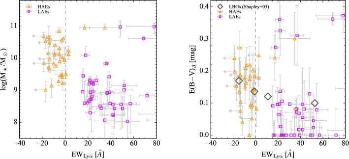
Figure 10: EW_Lyα vs. log stellar mass (a; left), E(B$-$V) derived from UV slope (b; right). The symbols are the same as shown in Fig. 8. The black diamonds in the right panel represent the results of composite spectra of Lyman break galaxies at $z\sim$3 reported by Shapley et al. (2003). Dashed vertical lines indicate EW${}_{\mathrm{Ly\alpha}}=0$ Å. To facilitate visualization, the figures only show the range of EW_Lyα between $-$40 and 80 Å.

Among 37 HAEs used in this paper, six objects show flux excesses in NB428 of which only two have significant  Ly$\alpha$ emission lines. The remaining 31 HAEs show no flux excesses in the NB428 image. Such a low fraction of LAEs well agrees with the past dual  Ly$\alpha$ and  H$\alpha$ emitter surveys (Hayes et al., 2010; Oteo et al., 2015; Matthee et al., 2016). Their  Ly$\alpha$ lines are either absent or in absorption (LAAs). In fact, such a high fraction of LAAs is expected from the past deep spectroscopic surveys (Shapley et al., 2003; Reddy et al., 2008; Hathi et al., 2016). Hathi et al. (2016) reported that about a half of UV luminous galaxies (i$<$25 mag) have EW_Lyα$<$0 Å and their median stellar mass is log(M_⋆/M_⊙)=9.65${}_{-0.02}^{+0.03}$. On the other hand, the median stellar mass of the HAEs is 10.12${}_{-0.59}^{+0.50}$, which suggests that the high fraction of LAAs in HAEs is probably due to older stellar populations in our HAE samples. In this section, we aim to interpret the origin of the  Ly$\alpha$ absorption. The uniqueness of this study is that our samples are selected so that they are limited by  H$\alpha$ line flux based on the narrow-band imaging at NIR, and hence independent of  Ly$\alpha$ line flux. They are widely spread in UV luminosities. Although the  Ly$\alpha$ narrow-band imaging cannot provide the spectrum of the  Ly$\alpha$ line directly, we can put constraints on EW_Lyα for individual galaxies even for UV faint objects (B$>25$ mag). Such measurements would be almost impossible with optical spectroscopy of a realistic observation time.

HAEs are expected to be located at $z$=2.50–2.55 whose  Ly$\alpha$ emission can be covered by the narrow-band filter NB428 (Fig. 1). One caution is that the NB2315 filter suffers from a small wavelength shift depending on the location of the detector as reported by Tanaka et al. (2011). The filter response curve shifts toward shorter wavelength up to $\sim$90 Å at the edge of the detectors, which may affect filter coverage of  Ly$\alpha$ line of HAEs at $z=2.5$. However, we think this effect is small, since Shimakawa et al. (2014) have identified that the HAEs discovered by the NB2315 filter in another field are confirmed to fall within the redshift interval of 2.50–2.54 by a follow-up spectroscopic survey. Therefore, the NB428 filter should neatly cover the wavelength range for  Ly$\alpha$ lines of our HAEs, and we do not take this effect into account in the following.

We investigate what physical properties such as SFRs, specific SFRs, and EW_Hα are related to EW_Lyα of HAEs. However, no clear relationship can be identified. In fact, the depth of the current narrow-band data is not enough to detect  Ly$\alpha$ absorption and put a constrain on EW_Lyα if it is smaller than $\sim-15$ Å. Unfortunately, this limitation does not allow us to study the physical meanings of the  Ly$\alpha$ absorption features in most of the HAEs, and we require much deeper narrow-band imaging for this purpose. However, we can compare our HAEs and LAEs in Fig. 10 where EW_Lyα is compared with (a) stellar masses on the left, and (b) dust reddening of UV continua on the right. Stellar masses and E(B$-$V) are derived from the SED-fitting and the UV slope as explained in §2.5. Moderate correlations can be seen in these plots.

We should note that narrow-band selected LAEs tend to be biased towards high EW_Lyα. However, these figures can easily tell us the differences between  H$\alpha$ and  Ly$\alpha$-flux limited samples; HAEs tend to be more massive and dustier than LAEs. Our HAEs seem to trace the EW_Lyα–E(B$-$V) relation found from the composite spectra of Lyman break galaxies at $z\sim$3 (Shapley et al. 2003, see also Cassata et al. 2015). This trend is also inferred from the anti-correlation between E(B$-$V) and the  Ly$\alpha$ photon escape fraction (Hayes et al., 2010; Matthee et al., 2016). We here note that a discrepancy between our LAE samples and LBGs (Shapley et al., 2003) at positive EW_Lyα should be due to a sample selection effect. The weak anti-correlation between E(B$-$V) and EW_Lyα can be interpreted as higher  Hi covering fraction for galaxies with higher dust extinction as suggested by Reddy et al. (2016b). However, this scenario cannot explain some outliers seen in the upper right corner of Fig. 10b. They show the reddest UV slopes, E(B$-$V) $>0.25$, and their locations are significantly deviated from the distributions of HAEs and LAEs on this diagram. Such a reverse trend has also been reported by Matthee et al. (2016), which find a bimodal relation in the UV slope versus the  Ly$\alpha$ photon escape fraction of HAEs at $z=2.2$. Those dusty LAEs would need another physical mechanism to emit strong  Ly$\alpha$ line emission such as galactic outflows powered by starbursts and/or AGNs (Mas-Hesse et al., 2003; Hashimoto et al., 2013; McLinden et al., 2014; Hayes, 2015; U et al., 2015). To confirm this hypothesis, follow-up spectroscopy is required.

4 Discussion

We have traced LAEs at $z=2.53$ down to the stellar mass of 10⁸ M_⊙ and SFR of 0.2 M_⊙/yr by deep narrow-band imaging as well as using publicly available various large surveys data (e.g. SXDS, CANDELS, 3D-HST). With this unique data-set, we investigate the yet-unexplored lower mass regime of the two major scaling relations at high redshifts; i.e., mass–SFR and mass–size relations. The results presented in the previous section suggest that the LAEs show no especially high or low star-forming activities for their stellar masses. Also their stellar sizes are neither particularly large nor particularly small for their masses when compared to the normal star-forming galaxies. These similarities are consistent at least in the low-mass regime, while massive LAEs seem to show distinctive physical properties at the same time. This section provides some further discussion on the results, including some concerns about the current analyses.

4.1 Similarities of physical properties in low-mass LAEs

This work has compared the physical properties of LAEs with those of HAEs at the same redshift, 2.5. Our results suggest that LAEs are less massive, less active, less dusty and younger galaxies than HAEs, and are smaller than more massive star-forming galaxies. However, for a given fixed stellar mass, they show no special characteristics in terms of SFR or size compared to other normal star-forming galaxies. This means that the LAE selection just picks out low-mass star-forming galaxies preferentially. Our selection is based on  Ly$\alpha$ luminosity,  Ly$\alpha$ equivalent width, and F160W-band magnitude. It can trace star-forming galaxies with stellar masses down to $\sim$10^8.5 M_⊙, if they are located on the linearly extrapolated main sequence of higher mass galaxies to the lower mass regime (Whitaker et al., 2014; Shivaei et al., 2015; Tomczak et al., 2016) (see §2.5 and §3.1).

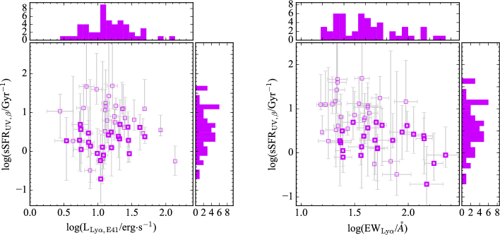
Figure 11: (a) The left panel shows  Ly$\alpha$ luminosity versus specific SFR derived from UV luminosity. (b) The right panel represents EW_Lyα versus specific SFR of LAEs at $z=2.5$. The SFRs are dust-corrected based on E(B$-$V) from the UV slope. The symbols are the same as in Fig. 8. Thick symbols indicate LAEs at M${}_{\star}\leq$10¹⁰ M_⊙ below the main sequence by Shivaei et al. (2015) shown in the Fig. 8b.

Figure 11 shows  Ly$\alpha$ luminosity and EW versus specific SFR (sSFR) of the LAEs. Thick symbols show less massive LAEs located below the main sequence of Shivaei et al. (2015). At the first sight, there are no strong trends in these diagrams, which suggests that enhanced star-forming activity is not required for the  Ly$\alpha$ photons to escape. Also, this indicates that our result is independent of the thresholds in  Ly$\alpha$ luminosity or EW. Therefore, star-forming activities may not be directly related to the escape mechanism of the  Ly$\alpha$ photons. There is actually a weak correlation between EW_Lyα and sSFR (Spearmans’s correlation coefficient of $-$0.39). This is probably due to the increased UV continua in high sSFR galaxies, and/or this would be partly caused by the observational limitation. As mentioned in §3.1, the narrow-band selection is insensitive to less active LAEs with low EW_Lyα, which depend on the depth of narrow-band and corresponding broad-band (B-band) images and the observed UV slopes of galaxies. Taking into account past studies (e.g. Yajima et al. 2012; Shibuya et al. 2014b; Reddy et al. 2016b), in principle the  Hi gas covering fraction and the dust obscuration are more likely to be controlling the  Ly$\alpha$ photon escape.

While the results suggest that the activity of star-formation does not play a critical role in the  Ly$\alpha$ escape, we still have a concern about interpreting the similarities in star-forming activities of LAEs on the mass–SFR diagram. The results of this work are based on the SFR calibration from UV luminosities and continuum slopes of LAEs, following the Kennicutt (1998); Meurer et al. (1999) prescriptions. This has a large uncertainty for young starburst populations, however, since the SFR estimations based on their calibrations are no longer valid as cautioned in their studies. The Kennicutt (1998) calibration assumes a continuous, constant star-formation rate over a timescale of 10⁸ yrs or longer. They also mention that this conversion tends to underestimate SFRs for very young star-forming galaxies. Wuyts et al. (2013) have reported a time dependence of the intrinsic  H$\alpha$/UV flux ratio for various star-formation histories (see Fig. 3 in their paper). For instance, they show that the intrinsic  H$\alpha$/UV ratio increases towards younger ages ($<$100 Myr) if a constant star-formation rate is assumed. (Cerviño et al., 2016) have reported in detail that the ratio of ionizing and non-ionizing photons strongly depends on the constituting stellar populations of different ages (Cerviño et al., 2016) determined by the star-formation histories. Therefore, even though galaxies have the same dust-corrected sSFR inferred from UV luminosities, they do not necessarily have the same amount of ionizing photons or  H$\alpha$ ( Ly$\alpha$) fluxes between the two cases. However, we cannot accurately derive  H$\alpha$ emission flux of LAEs with the NB2315 filter data alone, since the transmission curve of NB428 covers a wider redshift range than NB2315.

In short, this work suggests that  Ly$\alpha$ luminosities and equivalent widths do not necessarily correspond to star-forming activities at least in young low-mass galaxies ($<$10¹⁰ M_⊙), which is consistent with Hagen et al. (2016). Whereas, we should obtain more robust SFRs of LAEs independent of their star-formation histories, since those might have higher ionizing photons for a given sSFR inferred from UV luminosities. This factor is more important for SFR measurements of low-mass LAEs. There are actually low-mass star-forming galaxies at $z$$\sim$2 that have higher SFRs if  H$\alpha$ is used, than those measured from UV (Shivaei et al., 2015). Indeed, there is a possibility that  Ly$\alpha$ photons can more easily escape from less massive systems. In addition to that, this work does not use low-mass star-forming galaxies, which do not show  Ly$\alpha$ in emission for comparison. A direct comparison of the properties of LAEs and non-LAEs at the same low-mass regime would be required to understand the mechanism of  Ly$\alpha$ escape in detail. Therefore, the current results are at this stage too early to conclude that LAEs are in the phase of secular evolution as is typical for normal star-forming galaxies in this mass range. A deep  H$\alpha$ line imaging survey (e.g. Hayashi et al. 2016) enables us to trace low-mass star-forming systems that have been explored only by  Ly$\alpha$ emission so far, and to resolve such an issue. Last, our results are limited to EW${}_{\mathrm{Ly\alpha}}>15$ Å. The most serious bias in this work could be that the narrow-band imaging would miss the LAEs with low EW_Lyα. Thus, our sample may be missing UV luminous LAEs with low  Ly$\alpha$ luminosities like Lyman break galaxies. However, we stress that such a bias, if it presents, would rather strengthen our conclusion that high sSFR is not required for  Ly$\alpha$ photons to escape.

4.2 Surface mass densities at z=2.5

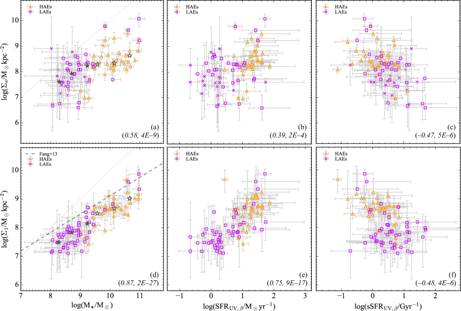
Figure 12: (a–c: from left to right in the upper part) Log stellar mass, dust-corrected SFR, and dust-corrected sSFR versus log effective mass surface density, (d–f: from left to right in the lower part) log stellar mass, dust-corrected SFR, and dust-corrected sSFR vs. log mass surface density within 1 kpc radius. The symbols are the same as shown in Fig. 9. Dotted lines on the left panels indicate log(M_⋆/M_⊙)= log($\Sigma_{\mathrm{e}}$/M_⊙kpc^-2) (a) and log($\Sigma_{\mathrm{1}}$/M_⊙kpc^-2) (d) for each diagram. The dashed line indicates the mass–$\Sigma_{\mathrm{1}}$ relation of green valley and red sequence galaxies at $z$$\sim$0, based on the GALEX-SDSS cross-matched sample (Fang et al., 2013). The Spearman’s rank correlation coefficients ($r$) and $p$ values are inset on lower left side in each diagram in the form of ($r$, $p$).

We investigate structure evolution of star-forming galaxies at $z$=2.5 based on the LAE and HAE samples. Figure 12a,c represent the surface density of stellar mass within effective radii ($\Sigma_{\mathrm{e}}$=M_⋆/2$\pi$R${}_{\mathrm{e}}^{2}$) and that within 1 kpc radii ($\Sigma_{\mathrm{1}}$) as a function of stellar mass. Because of the large errors on effective radii, $\Sigma_{\mathrm{e}}$ have large uncertainties in the low stellar mass range. $\Sigma_{\mathrm{1}}$ are derived from the SED fitting with fast (Kriek et al., 2009) based on the HST band photometries (F125,160W and F606,814,140W if available) within a fixed aperture radius of 1 kpc on a physical scale (0.3 arc sec diameter). Thus the $\Sigma_{\mathrm{1}}$ is computed from small aperture measurements, which stellar masses (M_⋆) are obtained for the whole galaxy. In the SED fitting, we set the same initial parameters as described in §2.5 assuming the delayed exponentially declining star-formation history.

If we limit our sample only to HAEs, we do not see any strong correlation between stellar mass and $\Sigma_{\mathrm{e}}$, while low-mass LAEs ($<10^{10}$ M_⊙) show a moderate positive relation between them (Spearman’s rank correlation coefficient is 0.37 corresponding to greater than 95% confidence level). On the other hand, we see an even tighter correlation between stellar mass and $\Sigma_{\mathrm{1}}$. The coefficient is 0.87 with more than 99.9 % confidence level for the combined sample of HAEs and LAEs. The distribution of galaxies of our sample on this diagram is consistent with other works such as Fang et al. (2013); Tacchella et al. (2015) for the local and $z$$\sim$2 star-forming galaxies, respectively. The positive correlations seen in these two diagrams offer the strong evidence for a vigorous mass growth in the early phase of galaxy formation. For massive galaxies above log(M_⋆/M_⊙)$\gtrsim$9.5, stellar mass – $\Sigma_{\mathrm{e}}$ relations are flattened and/or scattered. This suggests that the central part of galaxies is quickly built up and the inner mass density reaches to nearly a constant value as a function of mass (time). This indicates the inside-out growth of galaxy formation (Nelson et al., 2012, 2013, 2016b).

We confirm the existence of moderate or strong correlations of SFR and sSFR with mass surface densities ($\Sigma_{\mathrm{e}}$ and $\Sigma_{\mathrm{1}}$) (Fig. 12b,c,e,f) with the Spearman’s rank correlation coefficient of $r=0.39$ in $\Sigma_{\mathrm{e}}$–SFR, $r=-0.47$ in $\Sigma_{\mathrm{e}}$–sSFR, $r=0.75$ in $\Sigma_{\mathrm{1}}$–SFR, and $r=-0.48$ in $\Sigma_{\mathrm{1}}$–sSFR, respectively. The corresponding significance levels are more than 99.9%. However, such correlations disappear except for the $\Sigma_{\mathrm{1}}$–SFR relation, if we limit our sample to those with low surface densities $\lesssim$10⁸ M_⊙/kpc² (see also Franx et al. 2008; Whitaker et al. 2016). As the effective mass surface densities grow, star-forming activities characterised by the specific SFR tend to decline, while they tend to be more spread in SFRs (Fig. 12b,c). On the other hand, mass surface densities within 1 kpc strongly correlate with the total stellar masses and SFRs, and yet there is still a moderate anti-correlation between $\Sigma_{\mathrm{1}}$ and sSFR. Such a surface density effect is thought to be one of the major factors leading to a quenching of star formation activities (Franx et al. 2008; Fang et al. 2013; Omand et al. 2014; Woo et al. 2015; Whitaker et al. 2016, but see Lilly & Carollo 2016). This may be qualitatively consistent with the morphological/gravitational quenching (Martig et al., 2009; Davis et al., 2014; Genzel et al., 2014).

In section §3.1 and §3.2, we not only confirm the similarities of star-forming activities and size distributions of LAEs at the low-mass regime, but we now also find a possible uniqueness of massive LAEs which tend to be compact and less active for a given stellar mass. Fig. 12 exactly provides us with the combined information of these two results. Massive LAEs are located at the edge on the sSFR versus mass surface density diagrams in the meaning that they tend to be compact and less active. This trend becomes more prominent when we use SFR_UV,sed (with dust correction based on the SED-fitting) and SFR_SED (SED-inferred SFR). These less active massive LAEs would be post-starburst-like galaxies as discovered by Taniguchi et al. (2015), which might have experienced a nuclear starburst due to such major mergers and a subsequent quenching. Combined with a clear  Ly$\alpha$ escape seen in them, a favourable interpretation of such massive LAEs is that a nuclear starburst invokes a strong galactic outflow, which clears surrounding gas along the line of sight, and eventually allows  Ly$\alpha$ photons to escape. So far, we do not have a strong evidence for this hypothesis. Note that they do not have strong AGNs as they are not identified so by X-ray (Ueda et al., 2008) or MIPS 24$\mu$m (Dunlop et al., 2007) data.

In Table 3, we summarise the median values and 1 sigma scatters of dust-uncorrected SFRs (SFR_UV,obs), SFRs corrected for dust extinctions in several different ways (SFR_UV,β, SFR_UV,sed, and SFR_SED), effective radii (R_e), and mass surface densities within effective radii ($\Sigma_{\mathrm{e}}$) and those within 1 kpc radii ($\Sigma_{\mathrm{1}}$) for the LAEs in three different stellar mass bins ($<10^{8.5}$, $10^{8.5}$–$10^{9}$, and $10^{9}$–$10^{10}$ M_⊙).

Table 3: Median values and 1 sigma scatters of log SFR_UV,obs, SFR_UV,β, SFR_UV,sed, SFR_SED, R_e, $\Sigma_{\mathrm{e}}$, $\Sigma_{\mathrm{1}}$ of LAEs at $z=2.5$ in three different stellar mass bins ($<10^{8.5}$, $10^{8.5}$–$10^{9}$, and $10^{9}$–$10^{10}$ M_⊙).

log Stellar mass	8.30${}_{-0.16}^{+0.11}$	8.71${}_{-0.14}^{+0.18}$	9.24${}_{-0.16}^{+0.25}$
log SFRUV,obs	$-$0.05${}_{-0.33}^{+0.24}$	0.20${}_{-0.31}^{+0.30}$	0.30${}_{-0.39}^{+0.45}$
log SFRUV,β	0.19${}_{-0.49}^{+0.27}$	0.39${}_{-0.45}^{+0.54}$	0.75${}_{-0.75}^{+0.41}$
log SFRUV,sed	0.09${}_{-0.48}^{+0.69}$	0.46${}_{-0.51}^{+0.68}$	0.70${}_{-0.59}^{+0.53}$
log SFRSED	$-$0.27${}_{-1.31}^{+1.59}$	0.04${}_{-1.50}^{+1.39}$	0.56${}_{-0.70}^{+0.52}$
log Re	$-$0.01${}_{-0.37}^{+0.27}$	0.04${}_{-0.44}^{+0.64}$	0.11${}_{-0.22}^{+0.26}$
log $\Sigma_{\mathrm{e}}$	7.61${}_{-0.66}^{+0.64}$	7.93${}_{-1.38}^{+0.82}$	8.23${}_{-0.58}^{+0.57}$
log Stellar mass	8.28${}_{-0.15}^{+0.13}$	8.72${}_{-0.14}^{+0.18}$	9.24${}_{-0.16}^{+0.25}$
log $\Sigma_{\mathrm{1}}$	7.45${}_{-0.25}^{+0.19}$	7.84${}_{-0.41}^{+0.17}$	8.15${}_{-0.54}^{+0.41}$

4.3 Are the LAEs building blocks of local L* galaxies?

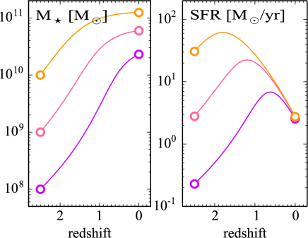
Figure 13: The predicted evolution in stellar mass (a; left) and SFR (b; right) of low-mass galaxies on the main sequence from $z$=2.5 to 0. Purple (top), pink (middle), and orange (bottom) curves indicate the evolutionary track from the initial masses of $1\times 10^{8}$, $10^{9}$, and $10^{10}$ M_⊙, respectively. Those growth histories are based on the assumption that the galaxies grow along the main sequence at each redshift. The main sequences as a function of redshift are derived from the prescription by Tomczak et al. (2016).

Another interesting question is whether the LAEs evolve into typical L* galaxies in the local Universe. Past clustering analyses suggest that LAEs at $z\sim 2$ can be the building blocks of local L* galaxies like the Milky Way (Gawiser et al., 2007; Guaita et al., 2010, 2011). We therefore perform an experiment to discuss how the mass of these low-mass LAEs grows in time (redshift) based on a simple assumption that they are forced to grow along the redshift-dependent main sequence. A similar test has been performed by Tomczak et al. (2016), but in this paper, we discuss much lower mass galaxies at high redshift than those in Tomczak et al. (2016).

Note that such an analytical simulation gives us only a rough estimate and the actual evolution would depend on galaxy mergers and/or quenching of star formation. In a merger case, the estimated masses would be lower limits, as mergers can grow their masses further. In a quenching case, some LAEs may well be quenched by now and would have been dropped from the main sequence. Furthermore, some galaxies would appear suddenly on the main sequence either from above or below the main sequence at their birth time. We do not take into account all these complicated processes, and thus the results presented here should be received with caution.

Nevertheless, under those assumptions, the stellar mass as a function of redshift can be presented by the following equation;

$$m_{t}(z)=m_{0}+\Sigma_{i=0}^{z}[(1-R(t_{z-z_{i}}))\times\psi(z_{i},m_{i})\times\delta t_{z-z_{i}}].$$ (1)

We set the initial redshift of $z_{0}$=2.5 and the time interval of $\Delta z=-0.1$. $m_{0}$ is the initial mass at $z=z_{0}=2.5$. $\delta t_{z-z_{i}}$ [yr] is the age interval from the redshift $z_{i}$ to $z$ when we have the total stellar mass of $m_{t}(z)$. $\psi(z_{i},m_{i})$ is SFR at the given stellar mass of $m_{i}$ and the redshift of $z_{i}$, assuming the redshift-dependent main sequence reported by ZFOURGE survey (Tomczak et al., 2016). We must caution that their prescription does not cover low-mass galaxies at $z>2$. However, we assume this model works well even for our lower mass LAEs since they follow the extrapolated main sequence line as shown in Fig. 8. The equation is the following (eq. 4 in their paper);

$$\log[\psi(z_{i},m_{i})] = s_{0}(z_{i})-\log[1+(m_{i}/M_{0}(z_{i}))^{-\gamma}]$$

$$s_{0}(z_{i}) = 0.448+1.220z_{i}-0.174z_{i}^{2}$$

$$\log[M_{0}(z_{i})] = 9.458+0.865z_{i}-0.132z_{i}^{2}$$

$$\gamma = 1.091.$$

$R(z_{i})$ indicates the mass return rate from stars to interstellar matter determined by the mass loss rate of massive stars (on a timescale less than $1\times 10^{8}$ yr), AGB stars, and type-Ia supernovae (the latter two are dominant in later phases). The mass return rate strongly depends on the assumed stellar initial mass function and it is also slightly dependent on the used model. For example, Moster et al. (2013) employs the mass return rate predicted by the stellar population synthesis model of Bruzual & Charlot (2003) with Chabrier (2003) IMF. This provides the mass return rate of 12% higher than that used in Segers et al. (2016) which is based on a different simple stellar population model of Wiersma et al. (2009). We use the former prescription, which gives the following equation (eq. 16 in Moster et al. 2013);

$$R(t_{z_{-}z_{i}})=0.05\ln[(t_{z-z_{i}}+3\times 10^{5})/3\times 10^{5}].$$

The result of this simple analytical simulation shows that LAEs found in this observation can grow to galaxies with several times $10^{10}$ M_⊙ (Fig. 12a). Figure 12b shows their SFR histories. This suggests that star-forming activities in low-mass galaxies at $m_{0}=1\times 10^{8}$ M_⊙ are modest and cannot exceed the SFR of 10 M_⊙/yr during their growth histories. The predicted main sequence has a nearly flat slope above $1\times 10^{10}$ M_⊙ at $z$=0, and SFRs are all similar irrespective of initial stellar masses.

As a result, this simulation shows that the Milky Way galaxy with a stellar mass of $6.4\pm 0.6\times 10^{10}$ M_⊙ (McMillan, 2011) can be a descendant of one of those LAEs with a stellar mass of $\sim 1\times 10^{8.5}$ M_⊙ at $z=2.5$. Some fraction of the low-mass LAEs at $z=2.5$ may evolve into local L* type galaxies like the Milky Way. On the other hand, HAEs with M${}_{\star}>10^{10}$ M_⊙ seem to have a potential to grow into very massive objects with M${}_{\star}>10^{11}$ M_⊙ if they retain substantial gas reservoirs until later times.

4.4 Ly$\alpha$ absorbers traced by narrow-band imaging

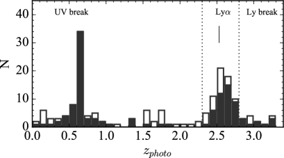
Figure 14: Photometric redshift distribution of the NB absorbers. We employ the best photometric redshifts ($z_{\mathrm{best}}$) in their catalogue. Filled and open histograms present the NB emitters with F160W$\leq$25 and F160W$>$25 mag, respectively. NB absorbers located at $z_{\mathrm{best}}$=2.3–2.8 are selected as  Ly$\alpha$ absorbers (LAAs).

Interestingly, a part of our HAE samples show  Ly$\alpha$ absorption rather than emission as shown in §3.3. The weak negative trend between E(B$-$V) and EW_Lyα is consistent with the past deep spectroscopic studies of Lyman Break galaxies at $z>2$ (Shapley et al., 2003; Cassata et al., 2013; Hathi et al., 2016) and agrees with the anti-correlation between E(B$-$V) and the  Ly$\alpha$ photon escape fraction reported by the past dual  H$\alpha$ and  Ly$\alpha$ emitter surveys (Hayes et al., 2010; Matthee et al., 2016) if we assume that the  Ly$\alpha$ EW is roughly comparable to the  Ly$\alpha$ photon escape fraction.

The fact that strong  Ly$\alpha$ absorption features in a part of HAEs indicates the potential use of narrow-band imaging to effectively search for  Ly$\alpha$-absorbed galaxies in narrow redshift slices by identifying the narrow-band flux deficits. In fact, this method is already demonstrated by Hayashino et al. (2004) in the familiar protocluster field, SSA22 at $z$=3.1 discovered by (Steidel et al., 1998). Here, we evaluate the availability of this technique again by incorporating the photometric redshift catalogue by 3D-HST (Momcheva et al., 2016) in the UDS-CANDELS field.

We first search for NB absorbers showing $3\sigma$ deficits in NB428 flux relative to B-band. We set the quite similar selection criteria as used for the identification of LAEs in this paper; (1) the colour cut of NB$-$B$>$0.476 mag corresponding EW${}_{\mathrm{Ly\alpha}}=-9$ Å in the rest frame at $z=2.53$, and the limiting magnitudes of $5\sigma$ in B band (27.89). For NB absorbers without narrow-band detections, 2$\sigma$ lower limit of NB magnitude are assumed (see also Appendix B).

Figure 14 presents photometric redshift distribution of obtained NB absorbers. The histogram suggests that this technique allows us to find  Ly$\alpha$ absorbers (LAAs) at $z$=2.5 quite effectively. The number of LAAs at photo-$z$ =2.3–2.8 is 65 is slightly larger than that of our LAE sample (50). The number ratio of LAAs to LAEs is roughly consistent with the result by recent deep spectroscopic survey (Hathi et al., 2016). Another spike seen at $z$$\sim$0.6 is due to UV break (B2640). A small difference of central wavelength between NB428 and B (170Å) allows us to detect this break feature (see Appendix B). The UV break around 2640 Å in the rest frame is known to be apparent in passive evolving galaxies (e.g. Cimatti et al. 2008). Indeed, we roughly check and confirm those red colours and spheroidal morphologies based on HST ACS/WFC3 images by visual inspection.

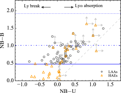
Figure 15: Colour-colour diagram between NB428$-$U and NB428$-$B. Black circles and orange triangles are  Ly$\alpha$ absorbers (LAAs) and HAEs, respectively (some of them overlap). Cross symbols show HAEs that cannot be seen in either NB428 and U bands, and thus those NB$-$U colours cannot be constrained at all. The blue solid horizontal line corresponds to the EW threshold of $\sim-$9 Å in the rest frame. The dash-dot and the dotted blue lines represent EW_Lyα=$-$15 and $-$20 Å, respectively. The grey dashed line indicates NB$-$U=NB$-$B.

We stress that the narrow-band deficits seen in LAAs should not be caused by Lyman Break feature at $\lambda$$<$1216 Å. Figure 15 show a colour-colour magnitude diagram of NB$-$U and NB$-$B. U-band filter covers the rest-frame wavelength of 955–1164 Å at $z$=2.53 which samples  Ly$\alpha$ forest continua. Thus U-band magnitude is basically fainter than B-band and narrow-band magnitudes due to absorption by intergalactic medium (IGM) in addition to dust reddening. For example, typical IGM transmission at $z$$\sim$2 is about 80% based on the calculation using BOSS  Ly$\alpha$ forest catalogue (Lee et al., 2013), which corresponds to absorption of $-$0.24 mag in U-band. Nevertheless, the figure shows that LAAs with larger  Ly$\alpha$ absorption EW (higher NB$-$B) tend to be redder even in NB$-$U colour, which indicates that the NB deficits in LAAs should be caused by  Ly$\alpha$ absorption. In particular, the HAE samples at $z$=2.5 selected independently by narrow-band observations at NIR also overlap with that of LAAs on this diagram. This strongly supports the fact that the NB deficits are caused by  Ly$\alpha$ absorptions rather than the Lyman break feature.

Such a strong  Ly$\alpha$ absorption is though to be due to high covering fraction (but not a unity) of  Hi clouds with high column densities N( Hi) $>10^{21}$ cm^-2. Reddy et al. (2016a, b) have shown the composite FUV spectrum of Lyman Break galaxies at $z\sim 3$, showing a blue-shifted  Ly$\alpha$ absorption feature due to the outflowing dense neutral hydrogen gas in the line of sight similar to what we see in some dwarf galaxies in the local Universe (Kunth et al., 1994; Atek et al., 2009a; Rivera-Thorsen et al., 2015). Another causal factor would be stellar  Ly$\alpha$ absorption, however, this may be cancelled out by  Ly$\alpha$ emission at least for star-forming galaxies according to the theoretical model by Peña-Guerrero & Leitherer (2013). Given the higher dust extinction of non-LAEs than that of LAEs (Hathi et al., 2016), the former case (higher  Hi covering fraction) seems to be the dominant factor, since the dust reddening is correlated to the  Hi covering fraction (Reddy et al., 2016b). We should note that our narrowband method could considerably underestimate  Ly$\alpha$ luminosity and EW_Lyα, depending on the locations of  Ly$\alpha$ emission or absorption with respect to the response curve of the narrowband filter. Complicated spectra at $\lambda\sim 1216$ Å including  Ly$\alpha$ emission and/or absorption prevent us from quantifying accurate  Ly$\alpha$ emissivities of galaxies only with the narrowband photometry. Therefore, we cannot rule out the possibility that these HAEs showing the narrowband deficits actually show  Ly$\alpha$ emission line as well.

A problem is that our narrow-band technique allows us to securely search for LAAs only with EW${}_{\mathrm{Ly\alpha}}<-9$ Å, and we are not able to detect the non-LAEs of course with the typical EW${}_{\mathrm{Ly\alpha}}\sim 0$ (Cassata et al., 2015; Hathi et al., 2016). Furthermore, ultra-deep narrow-band imaging is required to measure EW values of strong  Ly$\alpha$ absorbers by reaching the bottom of the line. Even if we conduct an observation with four times longer exposures (10 hrs), we would be able to constrain EW_Lyα only down to $-$20 Å in the rest frame. Considering these factors, the available EW_Lyα range with this method is actually quite limited. For example, our deep narrow-band observation can determine EW_Lyα in the range between $-9$ and $-15$ Å. This prevents us from studying the physical properties of LAAs over a range of  Ly$\alpha$ absorption strength comprehensively. This method, however, works well in searching for distant LAAs in a certain redshift slice, as demonstrated in this work.

4.5 Supplementary comments

Last, we complement the information about the LAE sample based on the narrow-band observations. However, note that it does not affect our main results or conclusions.

We also search for clumpy galaxies in the LAEs based on their WFC3/IR images. Our visual inspection finds only a few LAEs with multiple stellar components. This fraction is much smaller compared to the fraction of clumpy galaxies, $\sim$10–30% seen in UV bright galaxies at $z\sim 2$ (Shibuya et al., 2016), or $\sim$40% in Tadaki et al. (2014a). However, this difference may not be intrinsic, since we cannot resolve the internal structures of LAEs due to their intrinsically small sizes and their faintness.

To avoid a selection bias, this work does not exclude the mid-IR bright galaxy (LAE-31 in the Table 2) detected in the Spitzer UKIDSS Ultra Deep Survey (SpUDS; Dunlop et al. 2007). We also check the AGN population based on the catalogue by the Subaru/XMM-Newton Deep Survey (Ueda et al., 2008). However, we find no X-ray counterparts within 3 arcsec radius of each of the LAEs.

This work has presented that most of the HAEs do not show  Ly$\alpha$ line in emission. Rather, they sometimes show  Ly$\alpha$ line in absorption. On the flip side, Steidel et al. (2011) still find a diffuse  Ly$\alpha$ halo in the composite  Ly$\alpha$ narrow-band image of such  Ly$\alpha$-absorption systems. Matthee et al. (2016) also find diffuse  Ly$\alpha$ haloes in HAEs based on the dual  H$\alpha$ and  Ly$\alpha$ emitter surveys at $z=2.23$. In order to examine the presence of  Ly$\alpha$ halos in our HAE samples, we stack the  Ly$\alpha$ images of HAEs based on imcombine task of iraf by median, and then estimate  Ly$\alpha$ luminosity with different aperture diameter of 1.5, 2.0, 4.0, 6.0, and 8.0 arcsec with the SExtractor, which correspond to 9.9, 14.6, 31.5, 47.8, and 64.0 physical kpc, respectively. The composite  Ly$\alpha$ line image seems to be extended, since we find that  Ly$\alpha$ emission line luminosity roughly increases as L${}_{\mathrm{Ly\alpha}}=-3.72+0.49\times$(aperture diameter in arcsec) E41 erg/s. However, this luminosity growth is not significant if we take account of the errorbars. Therefore, we could not confirm a clear detection of  Ly$\alpha$ haloes with our data.

5 Conclusions

We have conducted an optical narrow-band imaging survey with the Suprime-Cam to search for LAEs at $z=2.5$ in the UDS-CANDELS field where we have already identified many HAEs in the same redshift slice by our previous narrow-band imaging survey at NIR. Together with existing WFC3/IR data from the HST and multi-band photometries from various large programs, we identify 50 LAE candidates at $z$=2.53 down to stellar mass of 10⁸ M_⊙and SFR of 0.2 M_⊙/yr. Our sample are limited by  Ly$\alpha$ luminosities ($>4.40\times 10^{41}$ erg/s in 1.5 arcsec aperture diameter),  Ly$\alpha$ equivalent widths ($>15$ Å), and H_F160W band magnitude ($<26.89$ mag). We combine 37 HAEs from our previous work (Tadaki et al., 2013), and investigate the physical properties of LAEs and HAEs such as their SFRs and sizes.

We compare star-forming activities and stellar angular sizes of LAEs with those of HAEs and other star-forming galaxies in the literature. The F160W/IR images for galaxies at $z=2.53$ are not affected by  H$\beta$ or  [Oiii] lines, which thus provide us with the accurate stellar masses and the sizes of the LAEs and HAEs. The depth of our narrow-band and B-band data allows us to explore star-forming galaxies with lower stellar masses down to $\gtrsim$10⁸ M_⊙. As a result, we find that LAEs follow the extrapolated line of the mass–SFR relation (star-forming main sequence) to the lower-mass end. The result is in good agreement with and complementary to Hagen et al. (2016) which have reported no difference between LAEs and controlled sample for comparison on the mass–SFR diagram at the similar redshift. The  Ly$\alpha$ luminosities and EWs do not strongly correlate with sSFR, indicating that star-forming activities do not contribute directly to the  Ly$\alpha$ photon escape mechanism. As suggested by recent studies (e.g. Yajima et al. 2012; Shibuya et al. 2014b; Reddy et al. 2016b), gas covering fraction and dust extinction would be the primary key factors. Indeed, we identify  Ly$\alpha$ absorption features in a part of the HAEs individually, which tend to be dustier and more massive systems.

Since NB428 filter can cover  Ly$\alpha$ emissions of the existing HAEs discovered by the past narrow-band (NB2315) imaging at NIR, the combination of these two narrow-band filter allow us to investigate  Ly$\alpha$ emissivities of HAEs. However, we detect significant flux excesses in only two HAEs. Six out of 37 HAEs have positive  Ly$\alpha$ EWs, of which 2 show significant  Ly$\alpha$ flux excesses at more than 3 sigma levels. Such a small fraction of LAEs among HAEs is consistent with the past similar studies (Hayes et al., 2010; Matthee et al., 2016), although it should be noted that the percentage should depend on the survey depths, photometric aperture size, physical properties of the parent HAE samples, and so on (Matthee et al., 2016). For example, photometric aperture size of 1.5 arcsec diameter used in this work is a half of that used in Matthee et al. (2016). We thus focus more on the  Ly$\alpha$ emissivity or its escape fraction along the line of sight.

Instead, we find flux deficits in the narrow-band for a larger fraction of our HAE sample. The flux-limited LAEs and HAEs are quite distinctively distributed on the EW_Lyα versus stellar mass or EW_Lyα versus E(B$-$V) diagrams. We conclude that LAEs have similar general properties as those of normal star-forming galaxies. However, they also remain as a unique population (low-mass young galaxies) because the majority of HAEs are not LAEs.

LAEs (low-mass star-forming galaxies) seem to share the same mass-size relation of massive star-forming galaxies within errors. On the other hand, four out of five massive LAEs at log(M_⋆/M_⊙)$>$9.5 have compact structures and are located close to the mass-size relation of early-type galaxies rather than that of late-type galaxies reported by van der Wel et al. (2014). Moreover, they have low sSFRs and high mass surface densities. Such massive LAEs have experienced nuclear starbursts in the past, which clear the surrounding gas by a galactic wind, allowing the  Ly$\alpha$ photon to escape from the systems as detected in our narrow-band  Ly$\alpha$ imaging.

Finally, we demonstrate the unique narrow-band technique to search for  Ly$\alpha$ absorbers (LAAs), which are observed as showing flux deficits in the narrow-band instead of flux excesses. Whilst this method can effectively trace LAAs in a certain redshift slice, we should note that the sample is limited to a narrow range of EW_Lyα in absorption due to observational limitations.

In order to generalise our results to normal star-forming galaxies, we will need to investigate other types of galaxy populations than LAEs at the same redshift and in the same stellar-mass range, and compare their physical properties with those of LAEs. We are now conducting systematic ultra-deep narrow-band imaging survey of low-mass, low-luminosity HAEs (Kodama et al.) for this purpose.

Appendix A Mass–SFR diagrams

The choice of SFR calibration among UV+IR, UV+E(B$-$V) and SED-fitting at UV–optical can affect the resultant slope of the main sequence. In particular, since the most dust obscured star-forming regions tend to be missing in the UV images and sometimes even in the optical images, the UV slopes of dusty objects are actually largely determined by outer regions, which are relatively more transparent due to small amounts of dust. This would then lead to an underestimation of E(B$-$V). In fact, recent spatially resolved analyses suggest a strong radial gradient in dust extinction in massive star-forming galaxies (Tadaki et al., 2014b; Nelson et al., 2016a; Tadaki et al., 2016) in the sense that galaxy centres have much heavier dust obscuration. Moreover, Tadaki et al. (2015) unveil the nuclear components hidden by dust in HAEs at $z>2$ by the spatially resolved dust continuum observations with Atacama Large Millimeter/submillimeter Array (ALMA). At the low-mass end, the surveys limited by ionizing photon flux (such as LAEs and HAEs) tend to miss post-starburst galaxies, which still show detectable UV luminosities. These factors would lead to the observed flatter main sequence based on  H$\alpha$.

The  H$\alpha$ luminosities with dust corrections by the Balmer decrement ( H$\alpha$ and  H$\beta$ ratio) provide the best, most accurate measurements of on-going SFR in the optical-to-NIR regime. This is largely independent of past star-formation histories, and relatively insulated from the influence of dust attenuation as compared to UV continuum. However, a part of the filter response curve of NB428 for  Ly$\alpha$ emission is not overlapped with that of NB2315 for  H$\alpha$ emission, unfortunately. This small mismatch prevents us from robustly estimating SFRs by  H$\alpha$ luminosities obtained from the narrow-band imaging data (Tadaki et al., 2013) for our LAEs.

Therefore, we carry out more comprehensive comparisons of the star-forming main sequence based on different recipes of dust corrections and SFR measurements other than  H$\alpha$-based one, such as SFRs derived from UV luminosities with dust correction by the UV slope (§2.5), the SED-fitting, or SFRs from full SED-fitting over a wide wavelength range. The latter method assumes the delayed exponentially declining star-formation histories and the other initial parameters are the same as §2.5. The results are shown in Fig. 16. Large error-bars associated to the SFR_SED of the LAEs are due to their faintness at all broad-band data as mentioned in §2.5. However, most of the measured SFRs are consistent with each other (Fig. 16c), and the median values agree with the main sequences presented for comparison which are obtained in the studies in the literature (Whitaker et al., 2014; Shivaei et al., 2015; Tomczak et al., 2016).

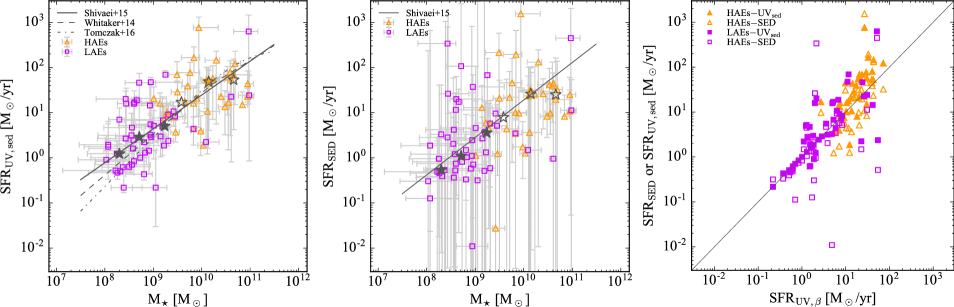
Figure 16: The stellar mass versus dust-corrected SFR, SFR_UV,sed where dust reddening is obtained from the SED-fitting (a: left) and the SED-based SFR, SFR_SED (b: middle). (c) The right panel compares SFR_UV,sed and SFR_SED with SFR_UV,β, which is used in the main body of this paper (Fig. 8). SFR_UV,β is derived from the UV luminosity with a dust correction based on the UV slope. The symbols are the same as in Fig. 8, but on the right panel, SFR_UV,β and SFR_SED are represented by filled and open symbols, respectively. Dashed, dot-dash, and solid lines represent the main sequences of the star-forming galaxies at $z$=2.0–2.5 reported by Whitaker et al. (2014), the one at $z$=2.5 from the prescription by Tomczak et al. (2016), and the one at $z$=2.0–2.6 by Shivaei et al. (2015), respectively. The SFR calibrations used in Whitaker et al. (2014) and Tomczak et al. (2016) is based on UV+IR luminosities. For the Shivaei et al. (2015) main sequence, we use their SFRs estimated in the same manner for each diagram for consistency. One should note that these works present the main sequence only for massive galaxies above $1\times 10^{9}$ or $1\times 10^{10}$ M_⊙ at $z\sim 2.5$. Here we just extrapolate their measured slopes to the lower mass galaxies.

Appendix B Selection of  Ly$\alpha$ Absorbers

This section provides supplementary information about the  Ly$\alpha$ absorption selection (§4.4). Figure 17 shows the colour–magnitude diagram for narrowband absorbers where stars with F160W$<$25 mag classified by the Skelton et al. (2014) catalogue have been removed. As described in the main text, we chose the absorbers showing more than $3\sigma$ deficits in their narrowband photometries with respect to those B-band magnitudes and have NB$-$B $>0.476$ mag and B $<27.89$ mag ($5\sigma$ limiting magnitude).

In order to select LAAs at $z=2.53\pm 0.03$, this work has employed photometric redshifts of the narrowband absorbers derived from the Momcheva et al. (2016) photo-$z$ catalogue based on the 3D-HST data. Also, we here investigate possible contaminations by using the single stellar population (SSP) model called GALAXEV (Bruzual & Charlot, 2003). The metallicities are fixed to the solar abundance, and no dust extinction is considered. The emission line components are not included.

The colour term distributions as a function of redshift are presented in Fig. 18. Our colour term correction ($+0.1$ mag) in §2.2 is reasonable considering the typical colour-term values of B$-$NB$\sim$$-$0.1 at $z<2.5$. Also, the simple models seem to be consistent with the observed colour terms of the photo-$z$ determined galaxies (Skelton et al., 2014; Momcheva et al., 2016) within the scatter. Slight downward offsets at $z>1.5$ would be due to strong dust attenuation in the FUV regime, since the central wavelength of the NB428 filter is slightly shorter by 170 Å than that of the B-band. At $z>2.5$, any absorption by the intergalactic medium (IGM) makes the B$-$NB colour bluer. Because of the difference in filter central wavelengths, a spectral break feature can also be captured by the narrowband selection. Especially, the UV break feature at around 2640 Å by old stellar populations with age $\geq 1$ Gyr is thought to be a main contamination as is actually seen in the photo-$z$ distribution of the narrow-band absorbers (Fig. 14). Although there are strong dips between the redshift 1 and 2 in the SSP model with the age of 2.5 and 0.9 Gyrs, these features would be negligible for our selection because those flux densities at the narrowband wavelength are much lower by two order of magnitude than those in the rest-frame optical.

We also see a dip in the colour-term distribution around $z=2.5$ due to the stellar  Ly$\alpha$ absorption. Galaxy spectra in the rest-frame FUV regime are mostly contributed from young massive stellar populations with the age younger than $\sim 100$ Myr (Bruzual & Charlot, 2003). The SSP models with the age of 25 and 100 Myrs show a significant narrow-band deficit due to a stellar  Ly$\alpha$ absorption at $z=2.5$, suggesting a possibility that our narrow-band selection may pick up this level of stellar absorption feature. In practice, however, such a young stellar population should also produce  Ly$\alpha$ line in emission, and this absorption feature may be filled up and disappear as simulated by Peña-Guerrero & Leitherer (2013) (see the main text in §4.4).

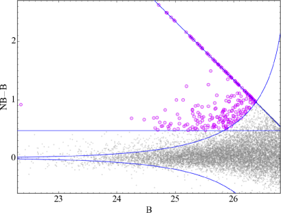
Figure 17: The colour-magnitude diagram of B vs. NB428$-$B. The grey dots show all the B-detected galaxies in the UDS-WFC3 field. The blue curves indicate the threshold of $\pm 3\sigma$ flux excess. The blue horizontal line indicates the criterion used for the equivalent width cut corresponding to EW${}_{\mathrm{rest}}=-9$ Å. The blue diagonal line indicates the 2$\sigma$ limit in B-band. The purple open circles show the NB selected absorbers that satisfy our selection criteria.

Figure 18: Colour term distributions of B$-$NB in the SSP models with various ages, 0.025, 0.1, 0.9, 2.5, and 11 Gyrs, plotted as a function of redshift. Those metallicities are fixed to the solar abundance. The downward arrow indicates the  Ly$\alpha$ redshift ($z=2.53$) for the narrow-band. The black open circles and the errorbars show the median values and the $1\sigma$ scatters of the photo-$z$ sources, respectively. Those photometric redshifts are taken from the Momcheva et al. (2016) catalogue ($z_{\mathrm{best}}$).

References

- Atek et al. (2008) Atek H., Kunth D., Hayes M., Östlin G., Mas-Hesse J. M., 2008, A&A, 488, 491
- Atek et al. (2009a) Atek H., Schaerer D., Kunth D., 2009a, A&A, 502, 791
- Atek et al. (2009b) Atek H., Kunth D., Schaerer D., Hayes M., Deharveng J. M., Östlin G., Mas-Hesse J. M., 2009b, A&A, 506, L1
- Barden et al. (2012) Barden M., Häußler B., Peng C. Y., McIntosh D. H., Guo Y., 2012, MNRAS, 422, 449
- Barro et al. (2013) Barro G., et al., 2013, ApJ, 765, 104
- Bertin & Arnouts (1996) Bertin E., Arnouts S., 1996, A&AS, 117, 393
- Bond et al. (2012) Bond N. A., Gawiser E., Guaita L., Padilla N., Gronwall C., Ciardullo R., Lai K., 2012, ApJ, 753, 95
- Brammer et al. (2012) Brammer G. B., et al., 2012, ApJS, 200, 13
- Bridge et al. (2013) Bridge C. R., et al., 2013, ApJ, 769, 91
- Bruzual & Charlot (2003) Bruzual G., Charlot S., 2003, MNRAS, 344, 1000
- Calzetti (2001) Calzetti D., 2001, PASP, 113, 1449
- Calzetti et al. (2000) Calzetti D., Armus L., Bohlin R. C., Kinney A. L., Koornneef J., Storchi-Bergmann T., 2000, ApJ, 533, 682
- Cassata et al. (2013) Cassata P., et al., 2013, A&A, 556, A68
- Cassata et al. (2015) Cassata P., et al., 2015, A&A, 573, A24
- Cerviño et al. (2016) Cerviño M., Bongiovanni A., Hidalgo S., 2016, A&A, 589, A108
- Chabrier (2003) Chabrier G., 2003, PASP, 115, 763
- Charlot & Fall (1993) Charlot S., Fall S. M., 1993, ApJ, 415, 580
- Cimatti et al. (2008) Cimatti A., et al., 2008, A&A, 482, 21
- Cirasuolo et al. (2010) Cirasuolo M., McLure R. J., Dunlop J. S., Almaini O., Foucaud S., Simpson C., 2010, MNRAS, 401, 1166
- Daddi et al. (2007) Daddi E., et al., 2007, ApJ, 670, 156
- Davis et al. (2014) Davis T. A., et al., 2014, MNRAS, 444, 3427
- Dawson et al. (2007) Dawson S., Rhoads J. E., Malhotra S., Stern D., Wang J., Dey A., Spinrad H., Jannuzi B. T., 2007, ApJ, 671, 1227
- Dunlop et al. (2007) Dunlop J., et al., 2007, A Spitzer Public Legacy survey of the UKIDSS Ultra Deep Survey, Spitzer Proposal
- Elbaz et al. (2007) Elbaz D., et al., 2007, A&A, 468, 33
- Fang et al. (2013) Fang J. J., Faber S. M., Koo D. C., Dekel A., 2013, ApJ, 776, 63
- Finkelstein et al. (2015) Finkelstein K. D., et al., 2015, ApJ, 813, 78
- Fitzpatrick (1999) Fitzpatrick E. L., 1999, PASP, 111, 63
- Foucaud et al. (2007) Foucaud S., et al., 2007, MNRAS, 376, L20
- Franx et al. (2008) Franx M., van Dokkum P. G., Förster Schreiber N. M., Wuyts S., Labbé I., Toft S., 2008, ApJ, 688, 770
- Furusawa et al. (2008) Furusawa H., et al., 2008, ApJS, 176, 1
- Gawiser et al. (2006) Gawiser E., et al., 2006, ApJ, 642, L13
- Gawiser et al. (2007) Gawiser E., et al., 2007, ApJ, 671, 278
- Genzel et al. (2014) Genzel R., et al., 2014, ApJ, 785, 75
- Grogin et al. (2011) Grogin N. A., et al., 2011, ApJS, 197, 35
- Guaita et al. (2010) Guaita L., et al., 2010, ApJ, 714, 255
- Guaita et al. (2011) Guaita L., et al., 2011, ApJ, 733, 114
- Hagen et al. (2014) Hagen A., et al., 2014, ApJ, 786, 59
- Hagen et al. (2016) Hagen A., et al., 2016, ApJ, 817, 79
- Hashimoto et al. (2013) Hashimoto T., Ouchi M., Shimasaku K., Ono Y., Nakajima K., Rauch M., Lee J., Okamura S., 2013, ApJ, 765, 70
- Hathi et al. (2016) Hathi N. P., et al., 2016, A&A, 588, A26
- Hayashi et al. (2012) Hayashi M., Kodama T., Tadaki K.-i., Koyama Y., Tanaka I., 2012, ApJ, 757, 15
- Hayashi et al. (2014) Hayashi M., et al., 2014, MNRAS, 439, 2571
- Hayashi et al. (2016) Hayashi M., Kodama T., Tanaka I., Shimakawa R., Koyama Y., Tadaki K.-i., Suzuki T. L., Yamamoto M., 2016, ApJ, 826, L28
- Hayashino et al. (2004) Hayashino T., et al., 2004, AJ, 128, 2073
- Hayes (2015) Hayes M., 2015, Publ. Astron. Soc. Australia, 32, e027
- Hayes et al. (2010) Hayes M., et al., 2010, Nature, 464, 562
- Hayes et al. (2013) Hayes M., et al., 2013, ApJ, 765, L27
- Hopkins & Beacom (2006) Hopkins A. M., Beacom J. F., 2006, ApJ, 651, 142
- Izotov et al. (2006) Izotov Y. I., Stasińska G., Meynet G., Guseva N. G., Thuan T. X., 2006, A&A, 448, 955
- Kashikawa et al. (2006) Kashikawa N., et al., 2006, ApJ, 648, 7
- Kashikawa et al. (2012) Kashikawa N., et al., 2012, ApJ, 761, 85
- Kennicutt (1998) Kennicutt Jr. R. C., 1998, ARA&A, 36, 189
- Kodama et al. (2004) Kodama T., Balogh M. L., Smail I., Bower R. G., Nakata F., 2004, MNRAS, 354, 1103
- Koekemoer et al. (2011) Koekemoer A. M., et al., 2011, ApJS, 197, 36
- Konno et al. (2016) Konno A., Ouchi M., Nakajima K., Duval F., Kusakabe H., Ono Y., Shimasaku K., 2016, ApJ, 823, 20
- Koyama et al. (2013) Koyama Y., Kodama T., Tadaki K.-i., Hayashi M., Tanaka M., Smail I., Tanaka I., Kurk J., 2013, MNRAS, 428, 1551
- Kriek et al. (2009) Kriek M., van Dokkum P. G., Labbé I., Franx M., Illingworth G. D., Marchesini D., Quadri R. F., 2009, ApJ, 700, 221
- Kunth et al. (1994) Kunth D., Lequeux J., Sargent W. L. W., Viallefond F., 1994, A&A, 282, 709
- Kunth et al. (1998) Kunth D., Mas-Hesse J. M., Terlevich E., Terlevich R., Lequeux J., Fall S. M., 1998, A&A, 334, 11
- Kusakabe et al. (2015) Kusakabe H., Shimasaku K., Nakajima K., Ouchi M., 2015, ApJ, 800, L29
- Laursen et al. (2013) Laursen P., Duval F., Östlin G., 2013, ApJ, 766, 124
- Lawrence et al. (2007) Lawrence A., et al., 2007, MNRAS, 379, 1599
- Lee et al. (2013) Lee K.-G., et al., 2013, AJ, 145, 69
- Leitherer & Heckman (1995) Leitherer C., Heckman T. M., 1995, ApJS, 96, 9
- Leitherer et al. (1999) Leitherer C., et al., 1999, ApJS, 123, 3
- Lilly & Carollo (2016) Lilly S. J., Carollo C. M., 2016, preprint, (arXiv:1604.06459)
- Malhotra & Rhoads (2002) Malhotra S., Rhoads J. E., 2002, ApJ, 565, L71
- Malhotra et al. (2012) Malhotra S., Rhoads J. E., Finkelstein S. L., Hathi N., Nilsson K., McLinden E., Pirzkal N., 2012, ApJ, 750, L36
- Martig et al. (2009) Martig M., Bournaud F., Teyssier R., Dekel A., 2009, ApJ, 707, 250
- Mas-Hesse et al. (2003) Mas-Hesse J. M., Kunth D., Tenorio-Tagle G., Leitherer C., Terlevich R. J., Terlevich E., 2003, ApJ, 598, 858
- Matthee et al. (2016) Matthee J., Sobral D., Oteo I., Best P., Smail I., Röttgering H., Paulino-Afonso A., 2016, MNRAS, 458, 449
- McLinden et al. (2014) McLinden E. M., Rhoads J. E., Malhotra S., Finkelstein S. L., Richardson M. L. A., Smith B., Tilvi V. S., 2014, MNRAS, 439, 446
- McMillan (2011) McMillan P. J., 2011, MNRAS, 414, 2446
- Meurer et al. (1999) Meurer G. R., Heckman T. M., Calzetti D., 1999, ApJ, 521, 64
- Miyazaki et al. (2002) Miyazaki S., et al., 2002, PASJ, 54, 833
- Moehler et al. (2014) Moehler S., et al., 2014, A&A, 568, A9
- Momcheva et al. (2016) Momcheva I. G., et al., 2016, ApJS, 225, 27
- Moster et al. (2013) Moster B. P., Naab T., White S. D. M., 2013, MNRAS, 428, 3121
- Nagamine et al. (2010) Nagamine K., Ouchi M., Springel V., Hernquist L., 2010, PASJ, 62, 1455
- Nakajima et al. (2012) Nakajima K., et al., 2012, ApJ, 745, 12
- Nakajima et al. (2013) Nakajima K., Ouchi M., Shimasaku K., Hashimoto T., Ono Y., Lee J. C., 2013, ApJ, 769, 3
- Nelson et al. (2012) Nelson E. J., et al., 2012, ApJ, 747, L28
- Nelson et al. (2013) Nelson E. J., et al., 2013, ApJ, 763, L16
- Nelson et al. (2016a) Nelson E. J., et al., 2016a, ApJ, 817, L9
- Nelson et al. (2016b) Nelson E. J., et al., 2016b, ApJ, 828, 27
- Nilsson & Møller (2011) Nilsson K. K., Møller P., 2011, A&A, 527, L7
- Nilsson et al. (2007) Nilsson K. K., et al., 2007, A&A, 471, 71
- Nilsson et al. (2011) Nilsson K. K., Östlin G., Møller P., Möller-Nilsson O., Tapken C., Freudling W., Fynbo J. P. U., 2011, A&A, 529, A9
- Noeske et al. (2007) Noeske K. G., et al., 2007, ApJ, 660, L43
- Oke & Gunn (1983) Oke J. B., Gunn J. E., 1983, ApJ, 266, 713
- Omand et al. (2014) Omand C. M. B., Balogh M. L., Poggianti B. M., 2014, MNRAS, 440, 843
- Oteo et al. (2012) Oteo I., et al., 2012, A&A, 541, A65
- Oteo et al. (2015) Oteo I., Sobral D., Ivison R. J., Smail I., Best P. N., Cepa J., Pérez-García A. M., 2015, MNRAS, 452, 2018
- Ouchi et al. (2004) Ouchi M., et al., 2004, ApJ, 611, 660
- Ouchi et al. (2008) Ouchi M., et al., 2008, ApJS, 176, 301
- Papovich et al. (2005) Papovich C., Dickinson M., Giavalisco M., Conselice C. J., Ferguson H. C., 2005, ApJ, 631, 101
- Peña-Guerrero & Leitherer (2013) Peña-Guerrero M. A., Leitherer C., 2013, AJ, 146, 158
- Peng et al. (2010) Peng C. Y., Ho L. C., Impey C. D., Rix H.-W., 2010, AJ, 139, 2097
- Reddy et al. (2008) Reddy N. A., Steidel C. C., Pettini M., Adelberger K. L., Shapley A. E., Erb D. K., Dickinson M., 2008, ApJS, 175, 48
- Reddy et al. (2016a) Reddy N. A., Steidel C. C., Pettini M., Bogosavljević M., 2016a, ApJ, 828, 107
- Reddy et al. (2016b) Reddy N. A., Steidel C. C., Pettini M., Bogosavljević M., Shapley A. E., 2016b, ApJ, 828, 108
- Rivera-Thorsen et al. (2015) Rivera-Thorsen T. E., et al., 2015, ApJ, 805, 14
- Sandberg et al. (2015) Sandberg A., Guaita L., Östlin G., Hayes M., Kiaeerad F., 2015, A&A, 580, A91
- Schaerer (2002) Schaerer D., 2002, A&A, 382, 28
- Schaerer (2003) Schaerer D., 2003, A&A, 397, 527
- Schlafly & Finkbeiner (2011) Schlafly E. F., Finkbeiner D. P., 2011, ApJ, 737, 103
- Segers et al. (2016) Segers M. C., Crain R. A., Schaye J., Bower R. G., Furlong M., Schaller M., Theuns T., 2016, MNRAS, 456, 1235
- Shapley et al. (2003) Shapley A. E., Steidel C. C., Pettini M., Adelberger K. L., 2003, ApJ, 588, 65
- Shen et al. (2003) Shen S., Mo H. J., White S. D. M., Blanton M. R., Kauffmann G., Voges W., Brinkmann J., Csabai I., 2003, MNRAS, 343, 978
- Shibuya et al. (2014a) Shibuya T., Ouchi M., Nakajima K., Yuma S., Hashimoto T., Shimasaku K., Mori M., Umemura M., 2014a, ApJ, 785, 64
- Shibuya et al. (2014b) Shibuya T., et al., 2014b, ApJ, 788, 74
- Shibuya et al. (2015) Shibuya T., Ouchi M., Harikane Y., 2015, ApJS, 219, 15
- Shibuya et al. (2016) Shibuya T., Ouchi M., Kubo M., Harikane Y., 2016, ApJ, 821, 72
- Shimakawa et al. (2014) Shimakawa R., Kodama T., Tadaki K.-i., Tanaka I., Hayashi M., Koyama Y., 2014, MNRAS, 441, L1
- Shimakawa et al. (2015a) Shimakawa R., Kodama T., Tadaki K.-i., Hayashi M., Koyama Y., Tanaka I., 2015a, MNRAS, 448, 666
- Shimakawa et al. (2015b) Shimakawa R., et al., 2015b, MNRAS, 451, 1284
- Shivaei et al. (2015) Shivaei I., et al., 2015, ApJ, 815, 98
- Skelton et al. (2014) Skelton R. E., et al., 2014, ApJS, 214, 24
- Sobral et al. (2016) Sobral D., et al., 2016, preprint, (arXiv:1609.05897)
- Song et al. (2014) Song M., et al., 2014, ApJ, 791, 3
- Speagle et al. (2014) Speagle J. S., Steinhardt C. L., Capak P. L., Silverman J. D., 2014, ApJS, 214, 15
- Stark et al. (2010) Stark D. P., Ellis R. S., Chiu K., Ouchi M., Bunker A., 2010, MNRAS, 408, 1628
- Steidel et al. (1998) Steidel C. C., Adelberger K. L., Dickinson M., Giavalisco M., Pettini M., Kellogg M., 1998, ApJ, 492, 428
- Steidel et al. (2011) Steidel C. C., Bogosavljević M., Shapley A. E., Kollmeier J. A., Reddy N. A., Erb D. K., Pettini M., 2011, ApJ, 736, 160
- Suzuki et al. (2015) Suzuki T. L., et al., 2015, ApJ, 806, 208
- Tacchella et al. (2015) Tacchella S., et al., 2015, Science, 348, 314
- Tadaki et al. (2013) Tadaki K.-i., Kodama T., Tanaka I., Hayashi M., Koyama Y., Shimakawa R., 2013, ApJ, 778, 114
- Tadaki et al. (2014a) Tadaki K.-i., Kodama T., Tanaka I., Hayashi M., Koyama Y., Shimakawa R., 2014a, ApJ, 780, 77
- Tadaki et al. (2014b) Tadaki K.-i., et al., 2014b, ApJ, 788, L23
- Tadaki et al. (2015) Tadaki K.-i., et al., 2015, ApJ, 811, L3
- Tadaki et al. (2016) Tadaki K.-i., et al., 2016, preprint, (arXiv:1608.05412)
- Tanaka et al. (2011) Tanaka I., et al., 2011, PASJ, 63, 415
- Taniguchi et al. (2015) Taniguchi Y., et al., 2015, ApJ, 809, L7
- Taylor (2005) Taylor M. B., 2005, in Shopbell P., Britton M., Ebert R., eds, Astronomical Society of the Pacific Conference Series Vol. 347, Astronomical Data Analysis Software and Systems XIV. p. 29
- Taylor (2015) Taylor M. B., 2015, in Taylor A. R., Rosolowsky E., eds, Astronomical Society of the Pacific Conference Series Vol. 495, Astronomical Society of the Pacific Conference Series. p. 177 (arXiv:1410.8507)
- Tomczak et al. (2016) Tomczak A. R., et al., 2016, ApJ, 817, 118
- Trainor et al. (2016) Trainor R. F., Strom A. L., Steidel C. C., Rudie G. C., 2016, preprint, (arXiv:1608.07280)
- U et al. (2015) U V., et al., 2015, ApJ, 815, 57
- Ueda et al. (2008) Ueda Y., et al., 2008, ApJS, 179, 124
- Vargas et al. (2014) Vargas C. J., et al., 2014, ApJ, 783, 26
- Verhamme et al. (2008) Verhamme A., Schaerer D., Atek H., Tapken C., 2008, A&A, 491, 89
- Verhamme et al. (2012) Verhamme A., Dubois Y., Blaizot J., Garel T., Bacon R., Devriendt J., Guiderdoni B., Slyz A., 2012, A&A, 546, A111
- Whitaker et al. (2014) Whitaker K. E., et al., 2014, ApJ, 795, 104
- Whitaker et al. (2016) Whitaker K. E., et al., 2016, preprint, (arXiv:1607.03107)
- Wiersma et al. (2009) Wiersma R. P. C., Schaye J., Theuns T., Dalla Vecchia C., Tornatore L., 2009, MNRAS, 399, 574
- Woo et al. (2015) Woo J., Dekel A., Faber S. M., Koo D. C., 2015, MNRAS, 448, 237
- Wuyts et al. (2013) Wuyts S., et al., 2013, ApJ, 779, 135
- Yabe et al. (2015) Yabe K., Ohta K., Akiyama M., Iwamuro F., Tamura N., Yuma S., Dalton G., Lewis I., 2015, ApJ, 798, 45
- Yagi et al. (2002) Yagi M., Kashikawa N., Sekiguchi M., Doi M., Yasuda N., Shimasaku K., Okamura S., 2002, AJ, 123, 66
- Yajima et al. (2012) Yajima H., Li Y., Zhu Q., Abel T., Gronwall C., Ciardullo R., 2012, ApJ, 754, 118
- van Dokkum (2001) van Dokkum P. G., 2001, PASP, 113, 1420
- van der Wel et al. (2012) van der Wel A., et al., 2012, ApJS, 203, 24
- van der Wel et al. (2014) van der Wel A., et al., 2014, ApJ, 788, 28