Distribution of Standard deviation of an observable among superposed states

Abstract

The standard deviation (SD) quantifies the spread of the observed values on a measurement of an observable. In this paper, we study the distribution of SD among the different components of a superposition state. It is found that the SD of an observable on a superposition state can be well bounded by the SDs of the superposed states. We also show that the bounds also serve as good bounds on coherence of a superposition state. As a further generalization, we give an alternative definition of incompatibility of two observables subject to a given state and show how the incompatibility subject to a superposition state is distributed.

1 Introduction

Quantum superposition is the most fundamental feature of quantum mechanics. Almost all the intriguing quantum phenomena are directly or indirectly related to quantum superposition. For example, it is the necessary factor for the interference of microscopic particles. In particular, combined with the tensor product structure of quantum state space, it can produce the most remarkable quantum phenomenon—–quantum entanglement which forms an important physical resource in quantum information processing [1]. However, the superposition in quantum mechanics does not always play the expected role. It could also lead to the coherent destruction. The obvious example is the vanishing entanglement for the superposition of two Bell states with equal amplitudes. So a natural question is how the entanglement is distributed among the different components of the superposition state or whether we can give a reference evaluation of the entanglement for the superposition state based on the entanglement of every component? This question was first addressed in Ref. [2], by Linden, Popescu and Smolin who found that the entanglement of superposition states (measured by the von Neumann entropy of reduced density matrix) was upper bounded in terms of the entanglement of each component. From then on, the entanglement of superposition states have attracted wide interests ranging from different bounds to various entanglement measures [3, 4, 5, 6, 7, 8, 9, 10, 11, 12, 13, 14, 15]. In addition, entanglement has been extensively studied in various systems [16] such as graphenes [17] and optomechanical systems [18] , and even in living object [19, 20]. The experimental preparation of quantum entanglement is also progressing fast [21, 22, 23, 24].

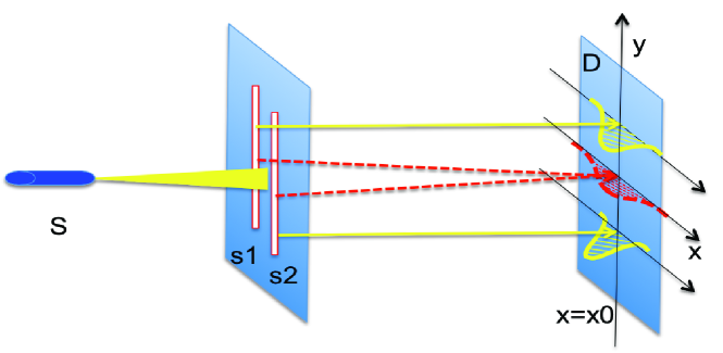
Figure 1: (Color online.)Diagrammatic sketch of double-slit experiment. The photon emitted from the coherent light source $S$ passes through two (or one of) slits $s1$ and $s2$ and is detected at position $x_{0}$ on the screen $D$. Along $y$ axis the SDs are shown at $x=x_{0}$ with different slits open. The yellow lines corresponds to the SD with only one slit open and the red line represents the SD with both slits open.

In practical physics, the measurement is the absolute requisite which allows us to know the objective world [25]. But any measurement is imperfect, so one has to perform repeated measurements to reduce the distance between the average result and the real value, that is, the measurement error. The standard deviation (SD) which quantifies the spread of the observed values on a measurement of an observable, is usually used to characterize the measurement error [26]. However, in the quantum world, besides the classical measurement errors, the quantum nature results in that measurements of an observable on the same quantum state don’t generally produce the same measurement value. So the SD also characterizes the essential uncertainty of a single measurement of an observable subject to a certain state. It further plays the important role in the remarkable Heisenberg’s uncertainty principle (see Ref. [27] and the references therein). It is also worth pointing out that the SD of observable in an ensemble has been used to distinguish ensembles with the same density matrix [28]. A related study can be also found in [29]. Since the superposition of states is a universal phenomenon in the quantum world, how is the SD distributed among the different components of the superposition states? Or how can we effectively evaluate the SD of the superposition state in terms of the SD of every component? For example, in a double-slit experiment shown in Fig. 1, suppose only one slit is open once, we can detect photon at a given position on the screen. Correspondingly, one can obtain the SDs of the position operator subject to each slit, respectively. Can we evaluate the SD at the same position in terms of the SD corresponding to each slit when both slits are open? In addition, since the usual uncertainly relation (or the incompatibility of observables) is given by the SDs of two incompatible observables, answering such a question could also provide a significant understanding on how the superposition influences the uncertainty relation.

In this paper, we answer the above questions by a general treatment in mathematics. It is found that the SD of the superposition state is well upper and lower bounded by the SDs of the superposed components. In addition, based on the formally consistent definitions of the SD and the coherence, it is interesting that the presented bounds on the SD can also serve as good bounds on coherence of the superposition state. That is, the bounds of the SD provide formally unified bounds on the SD and the coherence. Considering the connection with the uncertainty relation, we present an alternative incompatibility measure of two observables subject to a given state. It is shown that the bounds on the SD can also induce good bounds on the incompatibility of superposition states. The paper is organized as follows. In Sec. II, we present our main result about the bounds on the SD. In Sec. III, we provide the unified bounds on the coherence. In Sec. IV, we present the incompatibility measure of two observables and give its bounds. The conclusion is drawn finally.

2 Bounds on the standard deviation

To begin with, let’s consider an observable $A$ which is measured on a state $\left|\psi\right\rangle$. The SD is defined by

$$\Delta_{\psi}A=\sqrt{\left\langle A^{2}\right\rangle-\left\langle A\right\rangle^{2}},$$ (1)

where the subscript $\psi$ denotes that the expectation value $\left\langle X\right\rangle=\left\langle\psi\right|X\left|\psi\right\rangle$ for any observable $X$ is taken on the state $\left|\psi\right\rangle$. In the following, we also use $\left\langle X\right\rangle_{j}$ to denote $\left\langle\psi_{j}\right|X\left|\psi_{j}\right\rangle$ for some labeled state $\left|\psi_{j}\right\rangle$. Thus we suppose $\left|\psi\right\rangle$ is a superposition state, we aim to find how $\Delta_{\psi}A$ is bounded by the SDs of the superposed components. In this sense, we look for the bounds that can be expressed by the quantities directly related to the SD of every component instead of potentially tighter bounds given by other irrelevant quantities.

Theorem 1.-Let the observable $A$ be measured on the superposition state $\left|\psi\right\rangle=\sum\limits_{i=1}^{N}\alpha_{i}\left|\psi_{i}\right\rangle$ with $\sum\limits_{i=1}^{N}\left|\alpha_{i}\right|^{2}=1$ and $\left\|\left|\psi_{i}\right\rangle\right\|=1$, the SD $\Delta_{\psi}A$ can be bounded as

$$\mathcal{B}_{L}\leq\left\|\left|\psi\right\rangle\right\|^{2}\Delta_{\tilde{\psi}}^{2}A\leq\mathcal{B}_{U}$$ (2)

where $\left|\tilde{\psi}\right\rangle=\frac{1}{\left\|\left|\psi\right\rangle\right\|}$ $\left|\psi\right\rangle$ with $\left\|\left|\psi\right\rangle\right\|$ denoting the l₂ norm of a vector,

$$\mathcal{B}_{L}=\max\{0,b_{L}\}$$ (3)

with

$$b_{L}=\sum\limits_{i=1}^{N}\left|\alpha_{i}\right|^{2}\Delta_{{}_{\psi_{i}}}^{2}\left(A\right)-E_{+}(A)-F(A),$$ (4)

and

$$\mathcal{B}_{U}=\sum\limits_{i=1}^{N}\left|\alpha_{i}\right|^{2}\Delta_{{}_{\psi_{i}}}^{2}\left(A\right)-E_{-}(A)+F(A).$$ (5)

with

$$E_{\pm}(A)=\frac{\left(\left|\sum\limits_{i=1}^{N}\left|\alpha_{i}\right|^{2}\left\langle A\right\rangle_{i}\right|\pm\sum\limits_{i,j=1,i<j}^{N}2\left|\alpha_{i}\alpha_{j}\right|\sqrt{\left|\left\langle A\right\rangle_{i}\left\langle A\right\rangle_{j}\right|}\right)^{2}}{\left\|\left|\psi\right\rangle\right\|^{2}}+\sum\limits_{i=1}^{N}\left|\alpha_{i}\right|^{2}\left\langle A\right\rangle_{i},$$ (6)

and

$$F(A)=\sum\limits_{i,j=1,i<j}^{N}2\left|\alpha_{i}\alpha_{j}\right|\sqrt{\left(\Delta_{{}_{\psi_{i}}}^{2}\left(A\right)+\left\langle A\right\rangle_{i}^{2}\right)\left(\Delta_{{}_{\psi_{j}}}^{2}\left(A\right)+\left\langle A\right\rangle_{j}^{2}\right)}.$$ (7)

Proof. Based on the definition of the SD of $A$ on $\left|\psi\right\rangle$, we can have

$$\Delta_{\tilde{\psi}}^{2}\left(A\right) = \left\langle A^{2}\right\rangle_{\tilde{\psi}}-\left\langle A\right\rangle_{\tilde{\psi}}^{2}$$ (8)

$$= \frac{1}{\left\|\left|\psi\right\rangle\right\|^{2}}\left\langle A^{2}\right\rangle_{\psi}-\frac{1}{\left\|\left|\psi\right\rangle\right\|^{4}}\left\langle A\right\rangle_{\psi}^{2},$$

where the subscript denotes the expectation value on the corresponding state. Expanding $\left\langle A^{2}\right\rangle_{\psi}$, one arrives at

$$\left\langle A^{2}\right\rangle_{\psi}=\sum\limits_{i=1}^{N}\left|\alpha_{i}\right|^{2}\left\langle A^{2}\right\rangle_{i}+\sum\limits_{i,j=1,i\neq j}^{N}\alpha_{i}^{\ast}\alpha_{j}\left\langle A^{2}\right\rangle_{ij},$$ (9)

with $\left\langle X\right\rangle_{ij}=\left\langle\psi_{i}\right|X\left|\psi_{j}\right\rangle$ and $\left\langle X\right\rangle_{j}=\left\langle\psi_{j}\right|X\left|\psi_{j}\right\rangle$ for any observable $X$. Substitute Eq. (9) into Eq. (8), we will have

$$\left\|\left|\psi\right\rangle\right\|^{2}\Delta_{\tilde{\psi}}^{2}\left(A\right)$$ (10)

$$= \sum\limits_{i=1}^{N}\left|\alpha_{i}\right|^{2}\Delta_{{}_{\psi_{i}}}^{2}\left(A\right)+\sum\limits_{i=1}^{N}\left|\alpha_{i}\right|^{2}\left\langle A\right\rangle_{i}+\sum\limits_{i,j=1,i\neq j}^{N}\alpha_{i}^{\ast}\alpha_{j}\left\langle A^{2}\right\rangle_{ij}$$

$$- \frac{1}{\left\|\left|\psi\right\rangle\right\|^{2}}\left(\sum\limits_{i=1}^{N}\left|\alpha_{i}\right|^{2}\left\langle A\right\rangle_{i}+\sum\limits_{i,j=1,i\neq j}^{N}\alpha_{i}^{\ast}\alpha_{j}\left\langle A\right\rangle_{ij}\right)^{2}.$$

For an observable $X$, one can always find

$$\alpha_{i}^{\ast}\alpha_{j}\left\langle X\right\rangle_{ij}+\alpha_{i}\alpha_{j}^{\ast}\left\langle X\right\rangle_{ji}\leq 2\left|\alpha_{i}\alpha_{j}\right|\sqrt{\left|\left\langle X\right\rangle_{i}\left\langle X\right\rangle_{j}\right|},$$ (11)

which is based on the triangular inequality $\left|\sum a_{i}\right|\leq\sum\left|a_{i}\right|$ for numbers $a_{i}$ and Cauchy-Schwarz inequality. Eq. (10) will become

$$\left\|\left|\psi\right\rangle\right\|^{2}\Delta_{\tilde{\psi}}^{2}\left(A\right)$$ (12)

$$\geqslant \sum\limits_{i=1}^{N}\left|\alpha_{i}\right|^{2}\Delta_{{}_{\psi_{i}}}^{2}\left(A\right)+\sum\limits_{i=1}^{N}\left|\alpha_{i}\right|^{2}\left\langle A\right\rangle_{i}-\sum\limits_{i,j=1,i<j}^{N}2\left|\alpha_{i}\alpha_{j}\right|\sqrt{\left\langle A^{2}\right\rangle_{i}\left\langle A^{2}\right\rangle_{j}}$$

$$- \frac{\left(\left|\sum\limits_{i=1}^{N}\left|\alpha_{i}\right|^{2}\left\langle A\right\rangle_{i}\right|+\sum\limits_{i,j=1,i<j}^{N}2\left|\alpha_{i}\alpha_{j}\right|\sqrt{\left|\left\langle A\right\rangle_{i}\left\langle A\right\rangle_{j}\right|}\right)^{2}}{\left\|\left|\psi\right\rangle\right\|^{2}},$$

where we use the positivity property of $A^{2}$. Since Eq. (12) could be negative, but $\left\|\left|\psi\right\rangle\right\|^{2}\Delta_{\tilde{\psi}}^{2}\left(A\right)$ is never negative, we have to take the maximum between zero and the lower bound given by Eq. (12). Similarly, one can also obtain the upper bound from Eq. (10) as

$$\left\|\left|\psi\right\rangle\right\|^{2}\Delta_{\tilde{\psi}}^{2}\left(A\right)$$ (13)

$$\leq \sum\limits_{i=1}^{N}\left|\alpha_{i}\right|^{2}\Delta_{{}_{\psi_{i}}}^{2}\left(A\right)+\sum\limits_{i=1}^{N}\left|\alpha_{i}\right|^{2}\left\langle A\right\rangle_{i}+\sum\limits_{i,j=1,i<j}^{N}2\left|\alpha_{i}\alpha_{j}\right|\sqrt{\left\langle A^{2}\right\rangle_{i}\left\langle A^{2}\right\rangle_{j}}$$

$$- \frac{\left(\left|\sum\limits_{i=1}^{N}\left|\alpha_{i}\right|^{2}\left\langle A\right\rangle_{i}\right|-\sum\limits_{i,j=1,i<j}^{N}2\left|\alpha_{i}\alpha_{j}\right|\sqrt{\left|\left\langle A\right\rangle_{i}\left\langle A\right\rangle_{j}\right|}\right)^{2}}{\left\|\left|\psi\right\rangle\right\|^{2}}.$$

Here we use the triangular inequality $\left|a_{1}+a_{2}\right|\geqslant\left|\left|a_{1}\right|-\left|a_{2}\right|\right|$ for two numbers $a_{1}$ and $a_{2}$. Substitute $\left\langle A^{2}\right\rangle_{i}=\Delta_{{}_{\psi_{i}}}^{2}\left(A\right)+\left\langle A\right\rangle_{i}^{2}$ into Eq. (12) and Eq. (13), one will immediately obtain the bounds given in Eq. (3) and Eq. (5), which completes the proof. $\blacksquare$

From Theorem 1, one can find that whether the equality in Eq. (2) is achieved strongly depends on the considered observable $A$ and the superposed states. It can be shown that the equality saturates for two superposed states once one of the states happens to be the eigenvector of $A$ corresponding to its zero eigenvalue. In order to further show how tight the bounds are, we randomly generate a $4\times 4$ Hermitian operator

$$A=\left(\begin{array}[]{cccc}-1.3343&-0.7485&-0.5932&0.1623\\ -0.7485&0.2060&-0.0115&0.9184\\ -0.5932&-0.0115&-0.3338&0.3307\\ 0.1623&0.9184&0.3307&1.2613\end{array}\right)$$ (14)

and two 4-dimensional quantum states $\left|\psi_{1}\right\rangle=\left[\begin{array}[]{cccc}0.5506&0.3628&0.6016&0.4509\end{array}\right]^{T}$ and $\left|\psi_{2}\right\rangle=\left[\begin{array}[]{cccc}0.3511&0.4912&0.5296&0.5958\end{array}\right]^{T}$. The superposition state is given by $\left|\psi_{\pm}\right\rangle=x\left|\psi_{1}\right\rangle\pm\sqrt{1-x^{2}}\left|\psi_{2}\right\rangle$. We plot the upper and lower bounds and the SDs of the states $\left|\psi_{\pm}\right\rangle$ in Fig. 2 and Fig. 3. One can find from Fig. 2 that even though the lower bound is not so tight as the upper bound for $\left|\psi_{+}\right\rangle$, we still think the lower bound is also a tight bound, because in Fig. 3, with the same expressions of the bounds, the lower bound is much tighter than the upper bound for $\left|\psi_{-}\right\rangle$.

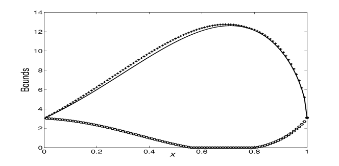
Figure 2: The upper and lower bounds and the SD of $\left|\psi_{+}\right\rangle$ versus $x$. The ’+’ line corresponds to the upper bound, the ’o’ line corresponds to the lower bound and the solid line is the SD of $\left|\psi_{+}\right\rangle$.

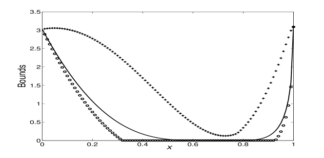
Figure 3: The upper and lower bounds and the SD of $\left|\psi_{-}\right\rangle$ versus $x$. The line styles are defined similar to Fig. 2.

3 Bounds on the coherence

Quantum coherence stemming from quantum superposition of states is the most fundamental feature of quantum mechanics. Recently, quantitative theory that captures the resource character has been developed [30], even though quantum coherence has been widely applied [31, 32, 33]. It pointed out that the good coherence measure should satisfy the following three conditions [30]: 1) Vanishing for incoherent states; 2) Not increasing under incoherent operations; 3) Not increasing under mixing of states. In fact, quantum coherence is also the essence of interference phenomena, which shows that no interference could be revealed by the observable if the observable commutes with the density matrix [31]. Here we would like to say that the quantum interference has also been extensively studied in [34], and resulted in the new concept of duality quantum computers, which has found striking advantage in the scaling of precision in quantum simulation [35]. Based on the commutation property, an interesting coherence measure, K-coherence, employing the skew information has been raised [36]. For a state $\varrho$, the K-coherence subject to an observable $K$ is defined by

$$I\left(\varrho,K\right)=-\frac{1}{2}Tr[\varrho^{1/2},K]^{2}.$$ (15)

It is especially noted that K-coherence depends not only on the measured state $\varrho$ but also on the observable $K$. If $K$ is degenerate, $I\left(\varrho,K\right)$ only detects the coherence in the non-degenerate subspace of $K$.

Now let’s turn to the SD $\Delta A$ of an observable $A$ subject to a pure state $\varrho=\left|\psi\right\rangle\left\langle\psi\right|$. It is easy to show that

$$\Delta_{\psi}A=\sqrt{I\left(\varrho,A\right)}=\sqrt{-\frac{1}{2}Tr[\varrho^{1/2},A]^{2}}$$ (16)

with $\varrho=\left|\psi\right\rangle\left\langle\psi\right|$ and $\left[\cdot,\cdot\right]$ denoting the commutation relation. This relation directly shows that the equivalence between the SD and the K-coherence for any an observable $A$ on a pure state. Thus one will easily obtain how the K-coherence is distributed among the superposed components.

Corollary 1.- For the superposition state $\left|\psi\right\rangle$ defined in Theorem 1, the K-coherence subject to the observable $A$ is bounded by

$$\mathcal{B}_{L}\leq\left\|\left|\psi\right\rangle\right\|^{2}I\left(\left|\tilde{\psi}\right\rangle\left\langle\tilde{\psi}\right|,A\right)\leq\mathcal{B}_{U}$$ (17)

where $\mathcal{B}_{L},\mathcal{B}_{U}$ have the same form in Theorem 1 but all the $\Delta_{\psi_{i}}A$ should be replaced by their corresponding $I\left(\left|\psi_{i}\right\rangle\left\langle\psi_{i}\right|,A\right)$.

Proof. This is a direct result of Eq. (16). $\blacksquare$

4 Bounds on the incompatibility

As mentioned at the beginning, the SD is the important ingredient for the remarkable Heisenberg uncertainty principle (HUP) [27]. However, the HUP is expressed in terms of the product of the SDs of two observables, so it could lead to a trivial bound even though two incompatible observables are taken into account [37]. Recently, Maccone and Pati [38] have raised another type of uncertainty relation by considering the sum of the SDs of two observables. They showed that the uncertainty relations would not get a trivial bound at any rate. It is natural that the nontrivial bound usually shows whether the considered observables are compatible or not. In fact, we would like to emphasize that the exact value of the sum of the SDs (or the exact value of the uncertainty) just signals to what degree the considered observables are incompatible. In this sense, we can define the incompatibility [39] of two operators $A$ and $B$ subject to a given normalized state $\left|\psi\right\rangle$ with $\left|\tilde{\psi}\right\rangle=\frac{\left|\psi\right\rangle}{\left\|\psi\right\|}$ as

$$U_{\psi}\left(A,B\right)=\Delta_{\tilde{\psi}}^{2}A+\Delta_{\tilde{\psi}}^{2}B.$$ (18)

It is obvious that $U_{\psi}\left(A,B\right)=0$ means that $A$ and $B$ can be simultaneously approximately measured on the state $\left|\tilde{\psi}\right\rangle$. The larger $U_{\psi}\left(A,B\right)$ is, the more incompatible $A$ and $B$. In addition, a reasonable (lower) bound for $U_{\psi}\left(A,B\right)$ could form an uncertainty relation. Now let’s consider when $\left|\psi\right\rangle$ is a superposition state, how the incompatibility can be distributed among every superposed component.

Corollary 2.-Let $\left|\psi\right\rangle$ be defined in Theorem 1, the incompatibility of two observable $A$ and $B$ $U_{\psi}\left(A,B\right)$ is bounded as

$$\tilde{\mathcal{B}}_{L}\leq\left\|\left|\psi\right\rangle\right\|^{2}U_{\tilde{\psi}}\left(A,B\right)\leq\tilde{\mathcal{B}}_{U}$$ (19)

with

$$\tilde{\mathcal{B}}_{L}=\max\{\tilde{b}_{L},0\},$$ (20)

where

$$\tilde{b}_{L}=\sum\limits_{i=1}^{N}\left|\alpha_{i}\right|^{2}U_{\psi_{i}}\left(A,B\right)-\sum\limits_{X=A,B}E_{+}(X)-\tilde{F}\left(A,B\right)$$ (21)

and

$$\tilde{\mathcal{B}}_{U}=\sum\limits_{i=1}^{N}\left|\alpha_{i}\right|^{2}U_{\psi_{i}}\left(A,B\right)-\sum\limits_{X=A,B}E_{-}(X)+\tilde{F}\left(A,B\right)$$ (22)

with

$$\tilde{F}\left(A,B\right) = \sum\limits_{i,j=1,i<j}^{N}2\left|\alpha_{i}\alpha_{j}\right|\sqrt{U_{\psi_{i}}\left(A,B\right)+\left\langle A\right\rangle_{i}^{2}+\left\langle B\right\rangle_{i}^{2}}$$ (23)

$$\times\sqrt{U_{\psi_{j}}\left(A,B\right)+\left\langle A\right\rangle_{j}^{2}+\left\langle B\right\rangle_{j}^{2}}$$

and $E_{\pm}(A)$ defined as Theorem 1.

Proof. For the observable $A$ and the state $\left|\psi\right\rangle$, we can obtain, from Theorem 1, the bounds of SD of $A$ as

$$\mathcal{B}_{L}(A)\leq\left\|\left|\psi\right\rangle\right\|^{2}\Delta_{\tilde{\psi}}^{2}A\leq\mathcal{B}_{U}(A)$$ (24)

where $\mathcal{B}_{L}(A)$ and $\mathcal{B}_{U}(A)$ with the same form as $\mathcal{B}_{L}$ and $\mathcal{B}_{U}$ just show that the bounds corresponds to the observable $A$. Similary, for $B$ we have

$$\mathcal{B}_{L}(B)\leq\left\|\left|\psi\right\rangle\right\|^{2}\Delta_{\tilde{\psi}}^{2}B\leq\mathcal{B}_{U}(B)$$ (25)

Sum Eq. (24) and Eq. (25), one will arrive at

$$\mathcal{B}_{L}(A)+\mathcal{B}_{L}(B) \leq \left\|\left|\psi\right\rangle\right\|^{2}U_{\tilde{\psi}}\left(A,B\right)$$ (26)

$$\leq \mathcal{B}_{U}(A)+\mathcal{B}_{U}(B)$$

Substitute Eq. (4) and Eq. (5) into Eq. (26), it can be found that

$$F(A)+F(B)$$ (27)

$$= \sum\limits_{i,j=1,i<j}^{N}2\left|\alpha_{i}\alpha_{j}\right|\sqrt{\left(\Delta_{{}_{\psi_{i}}}^{2}\left(A\right)+\left\langle A\right\rangle_{i}^{2}\right)\left(\Delta_{{}_{\psi_{j}}}^{2}\left(A\right)+\left\langle A\right\rangle_{j}^{2}\right)}$$

$$+\sum\limits_{i,j=1,i<j}^{N}2\left|\alpha_{i}\alpha_{j}\right|\sqrt{\left(\Delta_{{}_{\psi_{i}}}^{2}\left(B\right)+\left\langle B\right\rangle_{i}^{2}\right)\left(\Delta_{{}_{\psi_{j}}}^{2}\left(B\right)+\left\langle B\right\rangle_{j}^{2}\right)}$$

$$\leq \sum\limits_{i,j=1,i<j}^{N}2\left|\alpha_{i}\alpha_{j}\right|\sqrt{U_{\psi_{i}}\left(A,B\right)+\left\langle A\right\rangle_{i}^{2}+\left\langle B\right\rangle_{i}^{2}}$$

$$\times\sqrt{U_{\psi_{j}}\left(A,B\right)+\left\langle A\right\rangle_{j}^{2}+\left\langle B\right\rangle_{j}^{2}}$$

$$= \tilde{F}\left(A,B\right)$$

which is based on the Cauchy-Schwarz inequality. Thus one can easily find that the upper and lower bounds are given just as Eq. (21) and Eq. (22). The proof is completed. $\blacksquare$

5 Conclusion and discussion

We have derived an upper bound and a lower bound, respectively, for the SD of a superposition state in terms of the SDs of the superposed components. This lets us well understand how the SD is distributed among every superposed component. Numerical examples are given to test the tightness of the bounds. It is shown that such bounds can be well suitable for the distribution of the coherence of superposition states, since the coherence and the SD have the consistent form of definition based on the skew information. As a further connection with Heisenberg uncertainty principle, we suggest an alternative definition of incompatibility of two observables subject to a given state. Considering the superposition of state, we also study how we can evaluate the incompatibility of two observables subject to a superposition state in terms of the incompatibilities of every superposed component.

Since the SD is not the unique quantification of the uncertainty of the repeated measurement outcomes, it easily comes to our mind that the various entropy-based measure are also good candidates [40, 41, 42, 43, 44, 45, 46]. In particular, they don’t include the contribution of the eigenvalues of the observable. So how these types of measures are distributed among the different superposed components and what novel results could be implied in these relations deserve us forthcoming efforts.

6 Acknowledgements

This work was supported by the National Natural Science Foundation of China, under Grant No.11375036 and 11175033, the Xinghai Scholar Cultivation Plan and the Fundamental Research Funds for the Central Universities under Grant No. DUT15LK35 and No. DUT15TD47.

References

- [1] R. Horodecki, P. Horodecki, M. Horodecki, and K. Horodecki, Rev. Mod. Phys. 81, 865 (2009).
- [2] Noah Linden, Sandu Popescu and John A. Smolin, Phys. Rev. Lett. 97, 100502 (2006).
- [3] Chang-shui Yu, X. X. Yi and He-shan Song, Phys. Rev. A 75, 022332 (2007).
- [4] G. Gour, Phys. Rev. A 76, 052320 (2007).
- [5] D. Cavalcanti, M. Terra Cunha, and A. Acín, Phys. Rev. A 76, 042329 (2007).
- [6] J. Niset and N. J. Cerf, Phys. Rev. A 76, 042328 (2007).
- [7] Y.-C. Ou, Heng Fan, Phys. Rev. A 76, 022320 (2007).
- [8] J. Y. Xiang, S. J. Xiong, and F. Y. Hong, Eur. Phys. J. D 47, 257 (2008).
- [9] C. S. Yu, X. X. Yi, and H. S. Song, Eur. Phys. J. D 49, 273 (2008).
- [10] K.-H. Ma, C. S. Yu, and H. S. Song, Eur. Phys. J. D 59, 317 (2010).
- [11] S. J. Akhtarshenas, Phys. Rev. A 83, 042306 (2011).
- [12] P. Parashar and S. Rana, Phys. Rev. A 83 032301 (2011).
- [13] Amit Bhar, J. App. Maths. 2012, 1 (2012).
- [14] Amit Bhar, Ajoy Sen, and Debasis Sarkar, Quant. Inf. Proc. 12, 721 (2013).
- [15] Zhihao Ma, Zhihua Chen, and Shao-Ming Fei, Phys. Rev. A 90, 032307 (2014).
- [16] T. Zhou, Sci. China-Phys. Mech. Astron. 59, 640301 (2016).
- [17] C. Wang, W. W. Shen, S. C. Mi, et al., Sci. Bull. 60, 2016 (2015).
- [18] M. Gao, F. C. Lei, C. G. Du, et al., Sci. China-Phys. Mech. Astron. 59, 610301 (2016).
- [19] T. Li, Z. Q. Yin, Sci. Bull. 61(2), 163 (2016).
- [20] Qing A., Sci. Bull. 61(2),110 (2016).
- [21] R. Heilmann, M. Gräfe, S. Nolte, et al., Sci. Bull. 60, 96 (2015).
- [22] J. S. Xu, C. F. Li, Science Bulletin, 60, 141 (2015).
- [23] D. Y. Cao, B. H. Liu, Z. Wang, et al., Sci. Bull. 60, 1128 (2015).
- [24] Z. Wang, C. Zhang, Y. F. Huang, et al., Sci. Bull. 61, 714 (2016).
- [25] P. Busch, P. Lahti, and P. Mitteistaedt, The Quantum Theory of Measurement (2nd Edition Spinger-Verlag Berlin Heidelberg, 1996).
- [26] M. A. Nielsen and I. L. Chuang, Quantum Computation and Quantum Information (Cambridge University Press, Cambridge, 2000).
- [27] P. Busch, P. Lahti, and R. F. Werner, Rev. Mod. Phys. 86, 1261 (2014).
- [28] G. L. Long, Y. F. Zhou, J. Q. Jin, et al., Found. Phys. 36, 1217 (2006).
- [29] B. Chen, S.-M. Fei, Sci. Rep. 5, 14238 (2015).
- [30] T. Baumgratz, M. Cramer, and M. B. Plenio, Phys. Rev. Lett. 113,140401 (2014).
- [31] Marcelo O Terra Cunha, New J. Physics 9, 237 (2007).
- [32] Chang-shui Yu and He-shan Song, Phys. Rev. A 80, 022324 (2009).
- [33] Chang-shui Yu, Yang Zhang and Haiqing Zhao, Quant. Inf. Proc. 13(6),1437 (2014).
- [34] G.-L. Long. Comm. Theo. Phys. 45, 825 (2006).
- [35] S. J. Wei, G. L. Long, Quant. Inf. Proc. 15, 1189 (2016).
- [36] D. Girolami, Phys. Rev. Lett. 113, 170401 (2014).
- [37] Y. Watanabe, Formulation of Uncertainty Relation Between Error and Disturbance in Quantum Measurement by Using Quantum Estimation Theory (Springer Theses, Japan, 2014).
- [38] L. Maccone and Arun K. Pati, Phys. Rev. Lett. 113, 260401 (2014).
- [39] The incompatibility of two observables are usually described by their commutation relation, which can be seen from ‘https://en.wikipedia.org/wiki/Observable’. Here we emphasize the incompatibility subject to a given state. That is, even though the two observables don’t commute with each other, they could be simultaneously precisely measured on some given state. We would like to say that the definition of the incompatibility is not unique. Which definition could lead to deep applications remains unknown. But the product of two SDs should not be a good candidate, because it will vanish even if only one of the two observables is precisely measured on the given state.
- [40] S. Wehner, and A. Winter, New J. Phys. 12, 025009 (2010).
- [41] D. Deutsch, Phys. Rev. Lett. 50, 631 (1983).
- [42] H. Maassen and J. B. M. Uffink, Phy. Rev. Lett. 60, 1103 (1988).
- [43] M. Tomamichel and R. Renner, R. Phys. Rev. Lett. 106, 110506 (2011).
- [44] P. J. Coles and M. Piani, Phys. Rev. A 89, 022112 (2014).
- [45] Ł. Rudnicki, Z. Puchała and K. Źyczkowski, Phys. Rev. A 89, 052115 (2014).
- [46] Jun Zhang, Yang Zhang, Chang-shui Yu,Jun Zhang, Quant. Inf. Proc. 14, 2239 (2015).