Unified theory of electron-phonon renormalization and phonon-assisted optical absorption

Abstract

We present a theory of electronic excitation energies and optical absorption spectra which incorporates energy-level renormalization and phonon-assisted optical absorption within a unified framework. Using time-independent perturbation theory we show how the standard approaches for studying vibronic effects in molecules and those for addressing electron-phonon interactions in solids correspond to slightly different choices for the non-interacting Hamiltonian. Our present approach naturally leads to the Allen-Heine theory of temperature-dependent energy levels, the Franck-Condon principle, the Herzberg-Teller effect, and to phonon-assisted optical absorption in indirect band gap materials. In addition our theory predicts sub-gap phonon-assisted optical absorption in direct gap materials, as well as an exponential edge which we tentatively assign to the Urbach tail. We also consider a semiclassical approach to the calculation of optical absorption spectra which simultaneously captures energy-level renormalization and phonon-assisted transitions and is especially suited to first-principles electronic structure calculations. We demonstrate this approach by calculating the phonon-assisted optical absorption spectrum of bulk silicon.

1 Introduction

The development of electronic structure methods for studying many-electron systems in solid-state physics, nanoscience, and materials science, represents a major success of computational condensed matter research during the past three decades [1, 2, 3]. As the efficiency, availability, and accuracy of electronic structure techniques improve, the study of electron-phonon interactions from first principles is also becoming more accessible, and is drawing increasing interest among researchers.

The electron-nuclear interaction is ubiquitous in the photophysics of solids. For example this interaction renormalizes the excitation energies [4], modifies the strength of optical transitions through phonon-assisted processes [5], and underpins intriguing phenomena such as the exponential Urbach tail [6]. Yet despite the fundamental theory of indirect absorption being laid down more than half a century ago [7, 8, 9], it was not until very recently that a first-principles calculation of phonon-assisted absorption appeared in the literature [10]. It took a similarly long period of time to combine first-principles techniques with the semiclassical theory of the temperature renormalization of band structures [4, 11, 12, 13, 14].

It is interesting to contrast these relatively rare solid-state calculations with the field of computational quantum chemistry. Here, established methods for calculating optical properties including the quantum motion of nuclei are implemented in widely-used software packages [15]. Due to the different length scales addressed in solid-state physics and quantum chemistry, the study of electron-nuclear interactions in these two areas has followed distinct evolutionary paths leading to the development of different terminology. In quantum chemistry we find references to potential energy surfaces, excited-state nuclear wavefunctions, and Franck-Condon factors [16], while in solid-state physics the nuclear motion is usually described in terms of a bosonic phonon field [17]. Yet since a truly first-principles approach should maintain its validity across the length scales, there should be no fundamental barrier to obtaining a unified description of the effects of quantum nuclear motion in molecules and solids.

Motivated by these simple considerations we set out to develop a unified conceptual framework for describing electronic excitations and optical absorption spectra. Ideally this new framework should encompass and connect the current methods used for studying small molecules and extended solids. In order to keep the presentation as general as possible, we start from the many-body Schrödinger equation for electrons and nuclei, and make no assumptions on the practical approximations required to address the electron many-body problem.

In order to describe electrons and nuclei on an equal footing we use time-independent perturbation theory [18]. This choice, which is at variance with standard approaches to the electron-phonon interaction in solids [5], is important in order to develop a unified framework. In addition this choice is useful for clarifying interesting aspects of the electron-phonon physics in solids which have been missed in the recent literature.

The choice of the non-interacting Hamiltonian in the perturbative expansion is not unique. We show how two distinct choices lead naturally to the “molecular picture” or to the “solid-state picture”. Having identified the non-interacting Hamiltonians we then obtain correction terms for the electron-nuclear states and energies in powers of the electron-phonon coupling in each case.

We then employ this power expansion to describe electronic transitions, specialising to the case of optical excitations in the visible/UV range (as opposed to e.g. vibrational infrared spectroscopy). This analysis allows us to establish that phonon-assisted indirect absorption in solids and the Herzberg-Teller effect in molecules stem from the same perturbative term. As a byproduct of our analysis we obtain the temperature renormalization of excitation energies in solids, sub-gap absorption both in direct and indirect-gap materials, and an exponential absorption edge similar to the Urbach tail. We also discuss a promising semiclassical approach for calculating phonon-assisted and vibron-assisted optical absorption in solids and molecules.

The manuscript is organised as follows. In section 2 we introduce the key quantities needed for describing the interaction between electrons and nuclei in molecules and solids. In section 3 we provide a heuristic discussion of how to include quantum nuclear effects in electronic structure calculations. This section allows us to review the concept of phonon-induced renormalization of band structures. In sections 4–8 we tackle phonon-assisted absorption and energy-level renormalization from the quantum mechanical viewpoint within perturbation theory. We investigate both molecules (section 5) and solids (sections 6–8). In section 9 we bring together the molecular picture and the solid-state picture and discuss a method of calculating optical absorption spectra including quantum nuclear effects across the length scales. A practical demonstration of the method is provided in section 10, where we calculate the energy-level renormalization and optical absorption spectrum of bulk silicon. In section 11 we discuss briefly some technical aspects concerning the electronic Hamiltonian. Finally in section 12 we summarize our main findings and offer our conclusions. In this section we also highlight the key results and equations of our work.

2 The joint electron-nuclear system: notation and key approximations

2.1 The electron many-body problem

We consider a system consisting of electrons and nuclei, and we use $r$ and $R$ to denote the entire sets of electronic coordinates ${\bf r}_{1},{\bf r}_{2},\dots,{\bf r}_{N}$ and nuclear coordinates ${\bf R}_{1},{\bf R}_{2},\dots,{\bf R}_{M}$, respectively. The Hamiltonian of this system is given by:

$${\mathcal{H}}=H_{e}^{R}(r)+T^{R}+W^{R},$$ (1)

with $T^{R}$ the nuclear kinetic energy operator, $W^{R}$ the nucleus-nucleus Coulomb repulsion, and the electronic Hamiltonian $H_{e}^{R}$ given by:

$$H_{e}^{R}(r)=T_{e}(r)+W_{e}(r)+V_{en}^{R}(r).$$ (2)

In this expression $T_{e}(r)$ is the electronic kinetic energy operator, $W_{e}(r)$ the electron-electron Coulomb repulsion, and $V_{en}^{R}(r)$ is the attractive Coulomb interaction between electrons and nuclei. For each set of nuclear coordinates $R$ the formal solutions of the time-independent Schrödinger equation associated with the Hamiltonian $H_{e}^{R}(r)$ are obtained by solving:

$$H_{e}^{R}|\Psi^{R}_{\alpha}\rangle=E^{R}_{\alpha}|\Psi^{R}_{\alpha}\rangle,$$ (3)

where $\alpha$ may refer to a discrete index or to a continuous variable. By construction the eigenstates $\Psi^{R}_{\alpha}(r)$ define a complete basis, ${\sum}_{\alpha}|\Psi^{R}_{\alpha}\rangle\langle\Psi^{R}_{\alpha}|=1$, where the sum should be understood as an integral in the case of continuous indices. Starting from the eigenenergies $E^{R}_{\alpha}$ we define the potential energy surface (PES) $U^{R}_{\alpha}$ in the electronic state $|\Psi^{R}_{\alpha}\rangle$, so as to make contact with the standard quantum chemistry literature:

$$U^{R}_{\alpha}=E^{R}_{\alpha}+W^{R}.$$ (4)

This quantity essentially describes the potential energy landscape seen by the nuclei when the electronic and nuclear subsystems are considered as completely decoupled, with the electrons occupying the quantum state $|\Psi^{R}_{\alpha}\rangle$. At this stage, (4) should be regarded merely as a formal definition. In anticipation of the following discussion of electronic excitations and optical transitions we also introduce the electron excitation energy $\varepsilon_{\alpha}^{R}$ corresponding to the Hamiltonian in (3):

$$\varepsilon^{R}_{\alpha}=E_{\alpha}^{R}-E_{0}^{R},$$ (5)

where the subscript “0” labels the electronic ground state, and we are considering neutral excitations. For notational convenience, in the following we will indicate the many-body electron eigenstates and the excitation energies obtained from (3) at the equilibrium nuclear coordinates $R=R_{0}$ as $\Psi_{\alpha}(r)$ and $\varepsilon_{\alpha}$, respectively (i.e. without explicitly indicating the superscript $R_{0}$).

Throughout the manuscript we will assume that the many-body electron wavefunctions $\Psi^{R}_{\alpha}(r)$ are already known or can be calculated within some reasonable approximation. In the simplest approach one could start from density-functional theory (DFT) [19] and represent both the electronic ground-state and excited states using Slater determinants of Kohn-Sham wavefunctions [20]. In this case the optical transitions would be described within the independent-particle approximation, and the excitation energies would correspond to differences between the Kohn-Sham eigenvalues of empty and occupied single-particle states. Alternatively one could use more advanced methods specifically designed to describe neutral excitations, such as time-dependent DFT [21], or the Bethe-Salpeter approach [22, 23, 24]. Similarly, in the case of quantum chemistry calculations there exist many options for calculating ground and excited states, from the coupled cluster method to multireference configuration interaction [25]. Time-dependent DFT is also a very popular choice in this area, mostly within the standard Casida formulation [26]. The conclusions of our work do not depend on the specific approximations made in order to solve the electron many-body problem. The only requirement is that the chosen methodology be capable of yielding a reasonable optical absorption spectrum at fixed nuclei.

2.2 Nuclear dynamics

In order to address nuclear dynamics it is convenient to start from the potential energy surfaces defined by (4). Using these surfaces we can introduce one nuclear Schrödinger equation for each electronic state $|\Psi_{\alpha}^{R}\rangle$:

$$\left(T^{R}+U^{R}_{\alpha}\right)|\chi_{\alpha n}\rangle=E_{\alpha n}|\chi_{\alpha n}\rangle.$$ (6)

Here the nuclear wavefunctions $\chi_{\alpha n}(R)$ carry both the index $\alpha$ which specifies the PES, and the index $n$ labelling the solutions of (6). It is important to keep in mind that (6) is merely a definition, and serves only as a starting point for the following analysis.

Despite its apparent simplicity, (6) conceals an important subtlety. The definition of the potential energy surface $U^{R}_{\alpha}$ through (4) requires that the label $\alpha$ can be used to uniquely identify one electronic state for different nuclear configurations $R$. This is only possible when the states are non-degenerate for all values of $R$. The crossing of PES at certain nuclear configurations, which are referred to as conical intersections in the quantum chemistry literature [27], require a separate discussion and will not be addressed here (see B.2).

For future reference, in the case of the electronic ground state (6) trivially becomes

$$\left(T^{R}+U_{0}^{R}\right)|\chi_{0n}\rangle=E_{0n}|\chi_{0n}\rangle.$$ (7)

The analytical solution of this equation proceeds from the expansion of $U_{0}^{R}$ in terms of nuclear displacements from their equilibrium coordinates $R_{0}$. By retaining terms up to quadratic order in the displacements and performing a linear transformation (A) we find the standard textbook result:

$$U_{0}^{R}=U^{R_{0}}_{0}+{\sum}_{\nu}\,\frac{1}{2}\,M_{p}\,\Omega_{\nu}^{2}\,x_{\nu}^{2},$$ (8)

where $x_{\nu}$ and $\Omega_{\nu}$ are the amplitude and frequency of a vibrational mode $\nu$, and $M_{p}$ is a reference mass (in the following $x_{\nu}$ and $\Omega_{\nu}$ will only be used in relation to the ground-state PES). The quadratic expansion in (8) corresponds to the standard harmonic approximation for the ground state PES. This approximation has been very successful in many important cases [28], therefore it will be assumed in the following. Accordingly we will consider temperatures well below the melting point of the solid or the dissociation energy of the molecule. The study of anharmonic corrections could be tackled using the approach described in [29], however it will not be considered here since the formalism developed below is already rather involved.

After substituting (8) into (7), the nuclear wavefunctions $\chi_{0n}(R)$ can be expressed as the product of one-dimensional quantum harmonic oscillators. In this case the state $|\chi_{0n}\rangle$ is completely described by the set of integer occupation numbers of each quantized vibrational mode (A). In the following the index $n$ in $|\chi_{0n}\rangle$ will be understood to indicate the entire set of vibrational quantum numbers $n_{\nu}$. In the chemistry and in the solid-state literature the quanta of vibrational energy are referred to as “vibrons” and “phonons”, respectively. In order to simplify the notation in the following we will use phonons to indicate such quanta, regardless of the system (molecule or solid).

3 Heuristic approach to phonon-induced renormalization: temperature dependence and Allen-Heine theory

In this section we analyse the effect of quantum nuclear dynamics on the electronic excitation energies from a heuristic viewpoint. A more rigorous theory and its connection with the present derivation will be given in section 6.

If the nuclei could be held immobile in the configuration $R$, then the optical absorption spectrum of the system introduced in section 2 would exhibit sharp peaks at the energies $\varepsilon^{R}_{\alpha}$. The modification of these energies arising from the motion of the nuclei around their equilibium configuration is referred to as “phonon-induced renormalization” and is discussed below.

If we assume that electronic transitions occur at fixed nuclear coordinates, then each configuration $R$ yields the excitation energies $\varepsilon^{R}_{\alpha}$. The probability of finding the nuclei in the configuration $R$ can be calculated in a first approximation using the nuclear wavefunctions in (7), and is given by $|\chi_{0n}(R)|^{2}$. Therefore the transition energy averaged over all possible nuclear configurations can be obtained as $\int dR|\chi_{0n}(R)|^{2}\varepsilon^{R}_{\alpha}$, that is by evaluating the expectation value:

$$\langle\varepsilon_{\alpha}\rangle_{n}=\langle\chi_{0n}|\varepsilon_{\alpha}^{R}|\chi_{0n}\rangle.$$ (9)

At finite temperature $T$ the nuclear quantum states $|\chi_{0n}\rangle$ will be occupied according to the Gibbs distribution law $\exp(-E_{0n}/{k_{\rm B}T})/Z$, where $Z={\sum}_{n}\exp(-E_{0n}/{k_{\rm B}T})$ is the partition function and $k_{\mathrm{B}}$ Boltzmann’s constant. Using these occupations we can evaluate the thermally-averaged excitation energy $\langle\varepsilon_{\alpha}\rangle_{T}$ as:

$$\langle\varepsilon_{\alpha}\rangle_{T}=\frac{1}{Z}\sum_{n}e^{-\frac{E_{0n}}{{k_{\rm B}T}}}\langle\chi_{0n}|\varepsilon_{\alpha}^{R}|\chi_{0n}\rangle.$$ (10)

The heuristic argument used to derive this equation has been named the “semiclassical Franck-Condon approximation” in Ref. [30]. The semiclassical approach has been used successfully in recent first-principles calculations [31, 32]. As we show in section 5, the same result (10) can be derived from the Franck-Condon theory.

Equation (10) is the starting point of the theory of temperature-dependent bandstructures developed by Allen and Heine [4]. In the Allen-Heine theory the evaluation of (10) proceeds through the expansion of the electronic excitation energies in powers of the nuclear displacements from equilibrium (see A for notation):

$$\varepsilon^{R}_{\alpha}=\varepsilon_{\alpha}+{\sum}_{\nu}\frac{\partial\varepsilon_{\alpha}}{\partial x_{\nu}}x_{\nu}+\frac{1}{2}{\sum}_{\nu\mu}\frac{\partial^{2}\varepsilon_{\alpha}}{\partial x_{\nu}x_{\mu}}x_{\nu}x_{\mu}+{\mathcal{O}}(x_{\nu}^{3}).$$ (11)

By inserting (11) into (10) and carrying out the integration and the summation we obtain (A):

$$\langle\varepsilon_{\alpha}\rangle_{T}=\varepsilon_{\alpha}+{\sum}_{\nu}\,\frac{\partial\varepsilon_{\alpha}}{\partial n_{\nu}}\left[n_{\mathrm{B}}(\Omega_{\nu},T)+\frac{1}{2}\right]+{\mathcal{O}}(x_{\nu}^{4}),$$ (12)

where $n_{\rm B}(\Omega_{\nu},T)=[\exp(\hbar\Omega_{\nu}/{k_{\rm B}T})-1]^{-1}$ is the Bose-Einstein distribution function (with $\hbar$ the Planck constant), and we introduced the electron-phonon coupling coefficient:

$$\frac{\partial\varepsilon_{\alpha}}{\partial n_{\nu}}=l_{\nu}^{2}\ \frac{\partial^{2}\varepsilon_{\alpha}}{\partial x_{\nu}^{2}},$$ (13)

with

$$l_{\nu}=\sqrt{\frac{\hbar}{2M_{p}\Omega_{\nu}}}.$$ (14)

We note that this coupling coefficient contains both the “Debye-Waller” and the “Fan” terms of the Allen-Heine theory [4].

For a single harmonic oscillator with frequency $\Omega_{\nu}$, at high temperature (${k_{\rm B}T}\gg\hbar\Omega_{\nu}$) (12) predicts a linear dependence on temperature, while at low temperature the characteristic zero-point effect becomes apparent. From (12) we see that the “zero-point renormalization” of the excitation energy is $(\partial\varepsilon_{\alpha}/\partial n_{\nu})/2$. In section 10 we use (12) to calculate the temperature correction to the direct and indirect gaps of silicon.

Calculations based on the Allen-Heine theory have been employed successfully to describe the temperature dependence of optical excitations in a number of materials [11, 13, 14, 31, 32, 33, 34, 35, 36, 37, 38, 39]. Nonetheless it is important to bear in mind that (10), which underpins the Allen-Heine theory, constitutes a semiclassical approximation. As a result, the Allen-Heine theory cannot resolve fine structures in optical spectra, and its accuracy is practically limited by the characteristic phonon energy of the system under consideration. This point will become more clear in sections 5.4 and 7.2, where we shall establish the connection between the semiclassical expression (10) and a fully quantum-mechanical description of the electron-nuclear system.

4 Perturbation theory: choice of the non-interacting Hamiltonian

Now we consider the complete Hamiltonian ${\mathcal{H}}$ of the joint electron-nuclear system, given in (1). We want to partition ${\mathcal{H}}$ into a non-interacting Hamiltonian $H_{0}$, for which exact formal solutions can be obtained, and perturbative corrections $\Delta H$, to be treated within time-independent perturbation theory.

A perturbation approach is meaningful only when the corrections $\Delta H$ are small compared to the non-interacting Hamiltonian $H_{0}$. This consideration leads naturally to two different choices for $H_{0}$, one for molecules and one for extended solids. We start with the case of molecules.

4.1 Non-interacting Hamiltonian and perturbation terms for molecules

In the case of molecules, defects in solids and Frenkel excitons, neutral excitations usually involve sizable variations of the electron density in a localized region of space, with a characteristic size of the order of a few bond lengths. In this case it is expected that the PES seen by the nuclei will be strongly dependent on the quantum state occupied by the electrons. This observation can be used to partition the complete Hamiltonian ${\mathcal{H}}$ as follows:

$${\mathcal{H}} = H_{0}^{\mathrm{m}}+\Delta H^{\mathrm{m}},$$ (15)

where “m” stands for “molecular”, and the non-interacting Hamiltonian $H_{0}^{\mathrm{m}}$ is given by:

$$H_{0}^{\mathrm{m}}=T^{R}+{\sum}_{\alpha}U^{R}_{\alpha}|\Psi_{\alpha}\rangle\langle\Psi_{\alpha}|.$$ (16)

In this expression the PES $U^{R}_{\alpha}$ is defined through (4), and $\Psi_{\alpha}(r)$ denotes a solution of (3) for the equilibrium coordinates $R=R_{0}$. By construction the exact solutions of the non-interacting Hamiltonian $H_{0}^{\mathrm{m}}$ are given by $|\alpha n^{\rm m}\rangle=|\Psi_{\alpha}\rangle|\chi_{\alpha n}\rangle$, with $|\chi_{\alpha n}\rangle$ a solution of (6). The exact eigenenergies of the non-interacting Hamiltonian are given by $E_{\alpha n}$ in (6). These properties can be verified directly by evaluating $H_{0}^{\mathrm{m}}|\alpha n^{\rm m}\rangle$. The factorized solution $|\alpha n^{\rm m}\rangle$ is nothing but a Born-Oppenheimer wavefunction [40].

By combining (1), (2), (4), (15) and (16), and using the completeness of the electronic states $|\Psi_{\alpha}\rangle$, we obtain the perturbative correction $\Delta H^{\mathrm{m}}$:

$$\Delta H^{\mathrm{m}}=\sum_{\alpha}\left[\left(\langle\Psi_{\alpha}|H_{e}^{R}|\Psi_{\alpha}\rangle-E_{\alpha}^{R}\right)|\Psi_{\alpha}\rangle\langle\Psi_{\alpha}|+\sum_{\beta\neq\alpha}\langle\Psi_{\beta}|H_{e}^{R}|\Psi_{\alpha}\rangle|\Psi_{\beta}\rangle\langle\Psi_{\alpha}|\right]\!\!.$$

(17)

In order to simplify the perturbation expansions in the following sections, it is useful to express the first term in the square brackets in terms of the off-diagonal matrix elements $\langle\Psi_{\beta}|H_{e}^{R}|\Psi_{\alpha}\rangle$. This can be accomplished by expanding $E_{\alpha}^{R}$ in (3) in powers of $\left(H_{e}^{R}-H_{e}^{R_{0}}\right)$ (B.1). We find:

$$\langle\Psi_{\alpha}|H_{e}^{R}|\Psi_{\alpha}\rangle-E_{\alpha}^{R}=-\sum_{\beta\neq\alpha}\frac{|\langle\Psi_{\beta}|H_{e}^{R}|\Psi_{\alpha}\rangle|^{2}}{E_{\alpha}-E_{\beta}}+{\mathcal{O}}(3).$$ (18)

Here and in the following the symbol ${\mathcal{O}}(n)$ means that the remaining terms are of the order of $\left(H_{e}^{R}-H_{e}^{R_{0}}\right)^{n}$. The rationale behind this expansion is discussed in B.3. If we define:

$$V_{\beta\alpha}^{R}=\langle\Psi_{\beta}|\left(H_{e}^{R}-H_{e}^{R_{0}}\right)|\Psi_{\alpha}\rangle,$$ (19)

we can rewrite (17) in the compact form:

$$\Delta H^{\mathrm{m}}=-\sum_{\alpha}\sum_{\beta\neq\alpha}\left[\frac{|V_{\beta\alpha}^{R}|^{2}}{E_{\alpha}-E_{\beta}}|\Psi_{\alpha}\rangle\langle\Psi_{\alpha}|-V_{\beta\alpha}^{R}|\Psi_{\beta}\rangle\langle\Psi_{\alpha}|\right]+{\mathcal{O}}(3).$$ (20)

We will use this expression in evaluating the perturbative corrections in sections 5.1 and 5.2.

4.2 Non-interacting Hamiltonian and perturbation terms for solids

In the case of an extended solid the choice of the non-interacting Hamiltonian made in the previous section is not optimal. For example, if we consider crystalline silicon and an excited state corresponding to a Wannier exciton extending over 5 nm, the charge density variation with respect to the ground state is less than $10^{-5}$ electrons/atom. Therefore, it is expected that the PES seen by the nuclei in this excited state will be essentially identical to that of the ground state.

Following this reasoning, it seems sensible to choose the non-interacting Hamiltonian so that its solutions only contain the nuclear wavefunctions $\chi_{0n}$ from (6), corresponding to the ground-state PES $U_{0}^{R}$. This can be achieved by partitioning the complete Hamiltonian ${\mathcal{H}}$ as follows:

$${\mathcal{H}} = H_{0}^{\mathrm{s}}+\Delta H^{\mathrm{s}},$$ (21)

where “s” stands for “solid-state”, and the non-interacting Hamiltonian $H_{0}^{\mathrm{s}}$ is:

$$H_{0}^{\mathrm{s}}=T^{R}+U^{R}_{0}+{\sum}_{\alpha}\varepsilon_{\alpha}|\Psi_{\alpha}\rangle\langle\Psi_{\alpha}|.$$ (22)

The exact solutions of this Hamiltonian are $|\alpha n^{\mathrm{s}}\rangle=|\Psi_{\alpha}\rangle|\chi_{0n}\rangle$, with energies $E_{\alpha n}^{\mathrm{s}}=\varepsilon_{\alpha}+E_{0n}$. Since $\varepsilon_{\alpha}=E_{\alpha}^{R_{0}}-E_{0}^{R_{0}}$ vanishes for $\alpha=0$, the solutions of $H_{0}^{\mathrm{s}}$ and $H_{0}^{\mathrm{m}}$ coincide in the ground state.

Given the non-interacting Hamiltonian $H_{0}^{\mathrm{s}}$ in (21), the associated perturbative correction reads:

$$\Delta H^{\mathrm{s}}=\Delta H^{\mathrm{m}}+\Delta H^{\mathrm{AH}}.$$ (23)

The term $\Delta H^{\mathrm{m}}$ is the same as in (17) and (20) for the molecular case, while the new term $\Delta H^{\mathrm{AH}}$ is given by:

$$\Delta H^{\mathrm{AH}}={\sum}_{\alpha}(\varepsilon_{\alpha}^{R}-\varepsilon_{\alpha})|\Psi_{\alpha}\rangle\langle\Psi_{\alpha}|.$$ (24)

The superscript “AH” stands for “Allen-Heine”, and is meant to indicate that this term will lead to the Allen-Heine theory of temperature-dependent band structures (section 7.2). Again noting that $\varepsilon^{R}_{0}=0$, the perturbation $\Delta H^{\mathrm{AH}}$ has no effect when the electrons are in their ground state.

5 Perturbative corrections to the non-interacting molecular Hamiltonian: Herzberg-Teller effect, Franck-Condon principle, and temperature dependence

We now derive the perturbative corrections to the energy and wavefunctions of the many-body electron-nuclear states $|\alpha n^{\rm m}\rangle$ and $|\alpha n^{\rm s}\rangle$ introduced in section 4. To this end we apply time-independent perturbation theory to the perturbations $\Delta H^{\mathrm{m}}$ and $\Delta H^{\mathrm{s}}$. B.1 provides a reminder of the general expressions for the perturbative expansions used below. In this section we start with the molecular Hamiltonian $H_{0}^{\mathrm{m}}$, while in sections 6–7 we consider the solid-state Hamiltonian $H_{0}^{\mathrm{s}}$.

5.1 Perturbation corrections to the energies

If we denote the exact energy of the joint electron-nuclear eigenstates of ${\mathcal{H}}$ by $E_{\alpha n}^{\rm e,m}$ (the superscript “e” standing for “exact”), using (109) and (20) we obtain:

$$E_{\alpha n}^{\rm e,m}=E_{\alpha n}-\sum_{\beta\neq\alpha}\left[\frac{\langle\chi_{\alpha n}|\,|V_{\alpha\beta}^{R}|^{2}\,|\chi_{\alpha n}\rangle}{E_{\alpha}-E_{\beta}}-\sum_{m}\frac{|\langle\chi_{\alpha n}|V_{\alpha\beta}^{R}|\chi_{\beta m}\rangle|^{2}}{E_{\alpha n}-E_{\beta m}}\right]+{\mathcal{O}}(3).$$

This expression leads to a natural formal definition of the adiabatic approximation: in the following we will use the term adiabatic approximation in order to indicate the replacement:

$$\sum_{m}\frac{|\langle\chi_{\alpha n}|V_{\alpha\beta}^{R}|\chi_{\beta m}\rangle|^{2}}{E_{\alpha n}-E_{\beta m}}\simeq\sum_{m}\frac{|\langle\chi_{\alpha n}|V_{\alpha\beta}^{R}|\chi_{\beta m}\rangle|^{2}}{E_{\alpha}-E_{\beta}}.$$ (26)

This approximation is equivalent to stating that the electronic excitation energy $E_{\alpha}-E_{\beta}$ is much larger than the characteristic vibrational energy. To see this let us consider first the simplest scenario, whereby the potential energy surfaces $U_{\alpha}^{R}$ and $U_{\beta}^{R}$ are shifted by a constant. In this case, using the harmonic approximation, the operator identities given in A, and a linear expansion of $V_{\alpha\beta}^{R}$ in the atomic displacements, one finds that the matrix elements on the numerator only couple terms differing by one vibrational quantum number. As a result we have $E_{\alpha n}-E_{\beta m}=E_{\alpha}-E_{\beta}\pm\hbar\Omega$, with $\Omega$ the characteristic frequency associated with the potential energy surfaces. In more complicated situations, whereby the surfaces $U_{\alpha}^{R}$ and $U_{\beta}^{R}$ differ by more than a constant, it is always possible to perform an expansion of $U_{\beta}^{R}-U_{\alpha}^{R}$ in powers of $R$, and express $\chi_{\beta m}$ in terms of the wavefunctions of $U_{\alpha}^{R}$ using perturbation theory. In this case the only terms appearing in the sum will be $m_{\nu}=n_{\nu}\pm 1$ (first-order expansion), $m_{\nu}=n_{\nu}\pm 2$ (second-order expansion), and so on, and the previous reasoning still applies. These observations show that (26) will hold whenever $|E_{\alpha}-E_{\beta}|\gg\hbar\Omega$, and hence corresponds to the usual statement of the adiabatic approximation (e.g. [4]).

Using the adiabatic approximation defined by (26) and the completeness relation $\sum_{m}|\chi_{\beta m}\rangle\langle\chi_{\beta m}|=1$, the term within the square brackets in (5.1) vanishes. This allows us to identify that term with a non-adiabatic correction to the non-interacting energy $E_{\alpha n}$, and rewrite (5.1) as:

$$E_{\alpha n}^{\rm e,m}=E_{\alpha n}+{\mathcal{O}}(3),\qquad\mbox{(a. a.)}$$ (27)

where “(a. a.)” stands for “adiabatic approximation” and reminds us that non-adiabatic terms are neglected. The most severe breakdown of (26) will occur in the presence of degenerate electronic states. In this case the non-adiabatic coupling can be large and lead to a breakdown of the straightforward factorization of electronic and nuclear states [27] (B.2).

5.2 Perturbation corrections to the states: the Born-Huang expansion

We now use (110) to expand the exact electron-nuclear state $|\alpha n^{\rm e,m}\rangle$ in terms of the non-interacting Born-Oppenheimer states $|\alpha n\rangle$:

$$|\alpha n^{\rm e,m}\rangle=|\Psi_{\alpha}\rangle|\chi_{\alpha n}\rangle+\sum_{\beta\neq\alpha}\sum_{m}\frac{\langle\chi_{\beta m}|V_{\beta\alpha}^{R}|\chi_{\alpha n}\rangle}{E_{\alpha n}-E_{\beta m}}|\Psi_{\beta}\rangle|\chi_{\beta m}\rangle+{\mathcal{O}}(2).$$ (28)

By working with the first order expansion we shall introduce errors of ${\mathcal{O}}(2)$ into the oscillator strengths. On the other hand, by expanding the squared matrix elements it can be shown that these ${\mathcal{O}}(2)$ terms only modify the strength of the zeroth order transition, and do not introduce any new features. If we now apply the adiabatic approximation (26) to the expansion in (28), we obtain:

$$|\alpha n^{\rm e,m}\rangle\!=\!\left[|\Psi_{\alpha}\rangle+\sum_{\beta\neq\alpha}\frac{V_{\beta\alpha}^{R}}{E_{\alpha}-E_{\beta}}|\Psi_{\beta}\rangle\right]\!|\chi_{\alpha n}\rangle+{\mathcal{O}}(2).\qquad\mbox{(a. a.)}$$ (29)

The expression within the brackets can be identified as the $R$-dependent electronic wavefunction $\Psi_{\alpha}^{R}$. Expanding $|\Psi_{\alpha}^{R}\rangle$ in powers of $\left(H_{e}^{R}-H_{e}^{R_{0}}\right)$ we obtain (B.1):

$$|\Psi_{\alpha}^{R}\rangle=|\Psi_{\alpha}\rangle+\sum_{\beta\neq\alpha}\frac{\langle\Psi_{\beta}|H_{e}^{R}|\Psi_{\alpha}\rangle}{E_{\alpha}-E_{\beta}}|\Psi_{\beta}\rangle+{\mathcal{O}}(2).$$ (30)

Hence we obtain the following general expression for the joint electron-nuclear state:

$$|\alpha n^{\rm e,m}\rangle=|\Psi_{\alpha}^{R}\rangle|\chi_{\alpha n}\rangle+{\mathcal{O}}(2).\qquad\mbox{(a. a.)}$$ (31)

The quantity $|\Psi_{\alpha}^{R}\rangle|\chi_{\alpha n}\rangle$ appearing in (31) is the leading term in the so-called Born-Huang expansion of the joint electron-nuclear wavefunction [40]. Therefore, our present analysis shows that the wavefunction $|\Psi_{\alpha}^{R}\rangle|\chi_{\alpha n}\rangle$ constitutes the first-order adiabatic approximation to the exact electron-nuclear wavefunction $|\alpha n^{\rm e,m}\rangle$ in molecules.

5.3 Transitions: Herzberg-Teller effect and Franck-Condon principle

The perturbative expansions obtained in sections 5.1 and 5.2 will now be employed in order to analyze the expressions for the optical absorption spectra of molecules. We consider an external driving perturbation $\Delta\cos(\omega t)$, for example a uniform and oscillating electric field. This field induces transitions between the eigenstates of ${\mathcal{H}}$. The energy $\hbar\omega$ is taken in the UV-Visible range, so that $\Delta$ can be considered to couple only to the electronic degrees of freedom, i.e. $\Delta=\Delta(r)$. We evaluate the transition rates $W_{\alpha n\rightarrow\beta m}^{\rm e,m}(\omega)$ using the Fermi golden rule (considering absorption only):

$$W_{\alpha n\rightarrow\beta m}^{\rm e,m}(\omega)=\frac{2\pi}{\hbar}|\langle\beta m^{\rm e,m}|\Delta|\alpha n^{\rm e,m}\rangle|^{2}\delta(E^{\rm e,m}_{\beta m}-E^{\rm e,m}_{\alpha n}-\hbar\omega).$$ (32)

Using (27) and (31) we can rewrite the rates in terms of the Born-Oppenheimer states $|\chi_{\alpha n}\rangle$ and $|\chi_{\beta m}\rangle$:

$$W_{\alpha n\rightarrow\beta m}^{\rm e,m}(\omega)=W_{\alpha n\rightarrow\beta m}^{\mathrm{HT}}(\omega)+{\mathcal{O}}(2,3),\qquad\mbox{(a. a.)}$$ (33)

having defined:

$$W_{\alpha n\rightarrow\beta m}^{\mathrm{HT}}(\omega)=\frac{2\pi}{\hbar}|\langle\chi_{\beta m}|P_{\beta\alpha}^{R}|\chi_{\alpha n}\rangle|^{2}\delta(E_{\beta m}-E_{\alpha n}-\hbar\omega),$$ (34)

and

$$P_{\beta\alpha}^{R}=\langle\Psi_{\beta}^{R}|\Delta|\Psi_{\alpha}^{R}\rangle.$$ (35)

The notation ${\mathcal{O}}(n,m)$ in (33) is used to indicate that the neglected terms are of order ${\mathcal{O}}(n)$ in the strength of the transition and ${\mathcal{O}}(m)$ in the energy. We refer to the quantity $W_{\alpha n\rightarrow\beta m}^{\mathrm{HT}}(\omega)$ in (34) as the Herzberg-Teller rate, since it includes the characteristic $R$-dependence of the transition matrix element $P_{\beta\alpha}^{R}$ known as the Herzberg-Teller effect [41].

The Herzberg-Teller rate can further be approximated by neglecting the dependence of the matrix element $P_{\beta\alpha}^{R}$ on the nuclear coordinates. This corresponds to retaining only the zeroth order term in the expansion of the joint electron-nuclear state in (28). We find:

$$W_{\alpha n\rightarrow\beta m}^{\rm e,m}(\omega)=W_{\alpha n\rightarrow\beta m}^{\mathrm{FC}}(\omega)+{\mathcal{O}}(1,3),\qquad\mbox{(a. a.)}$$ (36)

having defined:

$$W_{\alpha n\rightarrow\beta m}^{\mathrm{FC}}(\omega)=\frac{2\pi}{\hbar}|\langle\chi_{\beta m}|\chi_{\alpha n}\rangle|^{2}|P_{\beta\alpha}|^{2}\delta(E_{\beta m}-E_{\alpha n}-\hbar\omega),$$ (37)

with $P_{\beta\alpha}=P_{\beta\alpha}^{R_{0}}$. This expression is the well-known rate of optical transitions according to the Franck-Condon principle [16]. In (37) the electrons and nuclei are completely decoupled, and the intensity of the transition results from the product of the electronic matrix element $P_{\beta\alpha}$ and the overlap of the nuclear wavefunctions $\langle\chi_{\beta m}|\chi_{\alpha n}\rangle$. The replacement of the Herzberg-Teller matrix element $P_{\beta\alpha}^{R}$ by its zeroth-order approximation $P_{\beta\alpha}$ is known as the Condon approximation.

The present analysis shows that the Herzberg-Teller rate and the Franck-Condon rate both correspond to the adiabatic approximation of the exact transition rate, correct to second order in the excitation energies. The strength of the transition is correct to first order in the former, and to zeroth order in the latter.

5.4 Temperature dependence: Connection to the Allen-Heine theory

In this section we demonstrate the link between the Franck-Condon rate in (37) and the thermally-averaged excitation energy $\langle\varepsilon_{\alpha}\rangle_{T}$ introduced in (10). To this end we evaluate the total rate of transitions from the electronic ground state $\Psi_{0}$ to the excited state $\Psi_{\alpha}$, irrespective of the vibrational quantum number of the final state. The temperature enters via the thermal distribution of the initial state among the vibrational quantum states $\chi_{0n}$, as in (10):

$$W^{\mathrm{FC}}_{0\rightarrow\alpha}(\omega,T)=\frac{1}{Z}\sum_{n}e^{-\frac{E_{0n}}{{k_{\rm B}T}}}\,\sum_{m}W_{0n\rightarrow\alpha m}^{\mathrm{FC}}(\omega).$$ (38)

By using (37) in this expression we find:

$$W^{\mathrm{FC}}_{0\rightarrow\alpha}(\omega,T)=\frac{1}{Z}\sum_{n}e^{-\frac{E_{0n}}{{k_{\rm B}T}}}\sum_{m}\frac{2\pi}{\hbar}|\langle\chi_{\alpha m}|\chi_{0n}\rangle|^{2}|P_{\alpha 0}|^{2}\delta(E_{\alpha m}-E_{0n}-\hbar\omega).$$

We can analyze this rate by inspecting the frequency moments. Using (4), (5), (6), as well as the completeness of the states $\chi_{\alpha m}$, the first moment can be written as:

$$\langle\hbar\omega\rangle^{{\rm FC},0\rightarrow\alpha}_{T} = \int\!d\omega\,\hbar\omega\,W^{\mathrm{FC}}_{0\rightarrow\alpha}(\omega,T)\Big{/}\!\int\!d\omega\,W^{\mathrm{FC}}_{0\rightarrow\alpha}(\omega,T)$$ (39)

$$= \frac{1}{Z}\sum_{n}e^{-\frac{E_{0n}}{{k_{\rm B}T}}}\langle\chi_{0n}|\varepsilon_{\alpha}^{R}|\chi_{0n}\rangle=\langle\varepsilon_{\alpha}\rangle_{T},$$

having used (10) to obtain the last equality. This result indicates that the thermally-averaged excitation energy obtained heuristically in (10)–(12), which forms the basis for the Allen-Heine theory, corresponds to the first moment of the Franck-Condon lineshape.

The comparison between the Franck-Condon lineshape and the Allen-Heine approach of section 3 can be extended to the case of higher frequency moments [30]. The width of the lineshape can be obtained from the second moment $\langle\hbar^{2}\omega^{2}\rangle^{{\rm FC},0\rightarrow\alpha}_{T}$, and this quantity also matches the square of $\varepsilon_{\alpha}^{R}$ in the Allen-Heine approach, i.e.

$$\langle\hbar^{2}\omega^{2}\rangle^{{\rm FC},0\rightarrow\alpha}_{T}=\langle\varepsilon_{\alpha}^{2}\rangle_{T}=\frac{1}{Z}\sum_{n}e^{-\frac{E_{0n}}{{k_{\rm B}T}}}\langle\chi_{0n}|\left(\varepsilon_{\alpha}^{R}\right)^{2}|\chi_{0n}\rangle.$$ (40)

However, moving beyond the second moment introduces commutators between the kinetic energy operator and potential energy surfaces [30]. The analysis of frequency moments will be investigated in further detail in section 9.

In summary, the present analysis indicates that, on the one hand, the Allen-Heine approach outlined in section 3 can be rooted on a solid ground by starting from perturbation theory and invoking the Franck-Condon approximation. On the other hand, it also indicates that the Allen-Heine expression (12) represents only an average excitation energy. As a consequence, the Allen-Heine theory is inadequate for resolving fine structures in optical spectra or small energy differences, and caution should be used when comparing to experiment.

This section concludes our discussion of electron-vibration coupling in molecules; in sections 6–7 we will build on the results obtained so far to discuss electron-phonon coupling in solids.

6 Perturbative corrections to the non-interacting solid-state Hamiltonian: electron-phonon renormalization and Allen-Heine theory

In the previous section we applied perturbation theory to the non-interacting molecular Hamiltonian $H_{0}^{\mathrm{m}}$, and established the connection to the Herzberg-Teller and Franck-Condon expressions for optical absorption in molecules, (34) and (37). Now we repeat the perturbation theory analysis for the solid-state picture, starting from the non-interacting solid-state Hamiltonian $H_{0}^{\mathrm{s}}$ (22). In this section we establish the link between the perturbative corrections to the energy levels and the electron-phonon renormalization resulting from the Allen-Heine theory [4]. In section 7 we will investigate the perturbative corrections to the joint electron-nuclear wavefunctions, and analyse phonon-assisted absorption in solids.

6.1 Perturbation corrections to the energies

Similarly to section 5.1 we denote the exact energy of the joint electron-nuclear states of ${\mathcal{H}}$ by $E_{\alpha n}^{\rm e,s}$. Using (20)–(24) with (109) we find:

$$E_{\alpha n}^{\rm e,s} = E_{\alpha n}^{\rm s}+\Delta E_{\alpha n}^{\rm AH}+{\mathcal{O}}(3)$$ (41)

$$-\sum_{\beta\neq\alpha}\left[\frac{\langle\chi_{0n}||V_{\beta\alpha}^{R}|^{2}|\chi_{0n}\rangle}{E_{\alpha}-E_{\beta}}-\sum_{m}\frac{|\langle\chi_{0n}|V_{\alpha\beta}^{R}|\chi_{0m}\rangle|^{2}}{E_{\alpha}-E_{\beta}+E_{0n}-E_{0m}}\right],$$

where $\Delta E_{\alpha n}^{\mathrm{AH}}$ is given by:

$$\Delta E_{\alpha n}^{\rm AH}=\langle\chi_{0n}|\varepsilon_{\alpha}^{R}|\chi_{0n}\rangle-\varepsilon_{\alpha}+\!\sum_{m\neq n}\frac{\left|\langle\chi_{0m}|\varepsilon_{\alpha}^{R}+\left[\langle\Psi_{\alpha}|H_{e}^{R}|\Psi_{\alpha}\rangle-\!E_{\alpha}^{R}\right]|\chi_{0n}\rangle\right|^{2}}{E_{0n}-E_{0m}}.$$

The term appearing within square brackets in (41) is the solid-state counterpart of the non-adiabatic corrections already discussed for molecules [see (5.1)]. This term can be neglected when the vibrational contribution $E_{0n}-E_{0m}$ in the second term is small compared to the electronic excitation energy $E_{\alpha}-E_{\beta}$. This observation allows us to state a formal definition of the adiabatic approximation in solids as follows:

$$\sum_{m}\frac{|\langle\chi_{0n}|V_{\alpha\beta}^{R}|\chi_{0m}\rangle|^{2}}{E_{\alpha}-E_{\beta}+E_{0n}-E_{0m}}\simeq\sum_{m}\frac{|\langle\chi_{0n}|V_{\alpha\beta}^{R}|\chi_{0m}\rangle|^{2}}{E_{\alpha}-E_{\beta}}.$$ (43)

This approximation constitutes the analogue of (26) for the case of solids. Also in this case it is expected that (43) will hold for systems with an electronic energy gap on the electronvolt scale. Under this conditions the square brackets in (41) can safely be ignored.

6.2 The zero-point energy

The energy correction $\Delta E_{\alpha n}^{\rm AH}$ appearing in (6.1) can be written in a more intuitive form by recasting all the $R$-dependent quantities in terms of displacements along the vibrational eigenmodes of the system. By proceeding along the same lines as in (11)–(13) and using the algebra of ladder operators in A we obtain:

$$\Delta E_{\alpha n}^{\rm AH}= = \sum_{\nu}\,\frac{\partial\varepsilon_{\alpha}}{\partial n_{\nu}}\left(n_{\nu}+\frac{1}{2}\right)-\sum_{\nu}\frac{l_{\nu}^{2}}{\hbar\Omega_{\nu}}\left(\frac{\partial\varepsilon_{\alpha}}{\partial x_{\nu}}\right)^{\!\!2}+{\mathcal{O}}(x_{\nu}^{4}).$$ (44)

In order to reach this expression it is convenient to express the second sum in (6.1) using (18) and (19), and observe that the cross terms in the square modulus vanish since they couple $|\chi_{0n_{\nu}}\rangle$ with $|\chi_{0,n_{\nu}\pm 1}\rangle$ and $|\chi_{0,n_{\nu}\pm 2}\rangle$, respectively. If we define the zero-point renormalization $E^{\mathrm{ZP}}_{\alpha}$ as the part of the energy-correction independent of the phonon numbers $n_{\nu}$:

$$E^{\mathrm{ZP}}_{\alpha}=\frac{1}{2}\sum_{\nu}\,\frac{\partial\varepsilon_{\alpha}}{\partial n_{\nu}}-\sum_{\nu}\frac{l_{\nu}^{2}}{\hbar\Omega_{\nu}}\left(\frac{\partial\varepsilon_{\alpha}}{\partial x_{\nu}}\right)^{\!\!2},$$ (45)

we can rewrite (41) more compactly as:

$$E_{\alpha n}^{\rm e,s}=E_{\alpha n}^{\rm s}+E_{\alpha}^{\mathrm{ZP}}+\sum_{\nu}\frac{\partial\varepsilon_{\alpha}}{\partial n_{\nu}}n_{\nu}+{\mathcal{O}}(3).\qquad\mbox{(a. a.)}$$ (46)

This expression, which was derived using second-order perturbation theory starting from the many-body electron-nuclear wavefunctions, is similar but not identical to the Allen-Heine result (12). In fact our expression contains an additional contribution to the zero-point energy, that is the second term in (45). Such contribution arises from the second sum in (6.1), and is absent in the Allen-Heine theory since the latter neglects off-diagonal couplings between different vibrational wavefunctions.

So far first-principles as well as semiempirical calculations based on the Allen-Heine theory [11, 12, 14, 38] did not include the extra term in (45). However, it will be important for future calculations to establish the magnitude of this correction.

7 Perturbative corrections to the solid-state non-interacting Hamiltonian: zero-phonon absorption and phonon-assisted absorption

7.1 Perturbation corrections to the states and optical matrix elements

In order to obtain the optical transition rates we use Fermi’s golden rule as in section 5.3. The counterpart of (32) for solids is trivially:

$$W^{\rm e,s}_{\alpha n\rightarrow\beta m}(\omega) = \frac{2\pi}{\hbar}|\langle\beta m^{\rm e,s}|\Delta|\alpha n^{\rm e,s}\rangle|^{2}\,\delta(E^{\rm e,s}_{\beta m}-E^{\rm e,s}_{\alpha n}-\hbar\omega).$$ (47)

The perturbative corrections to the energies appearing in the delta function were obtained in section 6.1. Here we need to derive the perturbative expansion of the joint electron-nuclear wavefunctions in order to evalate the optical matrix elements $\langle\beta m^{\rm e,s}|\Delta|\alpha n^{\rm e,s}\rangle$. Using (20), (23) and (24) inside (110) we find:

$$|\alpha n^{\rm e,s}\rangle = |\alpha n^{\rm s}\rangle+\sum_{m\neq n}\frac{\langle\chi_{0m}|\varepsilon_{\alpha}^{R}|\chi_{0n}\rangle}{E_{0n}-E_{0m}}|\alpha m^{\rm s}\rangle$$ (48)

$$+\sum_{\beta\neq\alpha}\sum_{m}\frac{\langle\chi_{0m}|V_{\beta\alpha}^{R}|\chi_{0n}\rangle}{E_{\alpha}-E_{\beta}+E_{0n}-E_{0m}}|\beta m^{\rm s}\rangle+{\mathcal{O}}(2).$$

After replacing the expansion (48) inside the transition matrix elements we obtain:

$$\langle\beta m^{\rm e,s}|\Delta|\alpha n^{\rm e,s}\rangle=\Delta_{\alpha n,\beta m}^{\rm dir,NP}+\Delta_{\alpha n,\beta m}^{\rm dir,PA}+\Delta_{\alpha n,\beta m}^{\rm ind,NP}+\Delta_{\alpha n,\beta m}^{\rm ind,PA}+{\mathcal{O}}(2),$$ (49)

with the definitions:

$$\Delta_{\alpha n,\beta m}^{\rm dir,NP}=P_{\beta\alpha}\,\delta_{nm},$$ (50)

$$\Delta_{\alpha n,\beta m}^{\rm dir,PA}=P_{\beta\alpha}(1-\delta_{nm})\frac{\langle\chi_{0m}|(\varepsilon_{\alpha}^{R}-\varepsilon_{\beta}^{R})|\chi_{0n}\rangle}{E_{0n}-E_{0m}},$$ (51)

$$\Delta_{\alpha n,\beta m}^{\rm ind,NP}=\delta_{nm}\left[\sum_{\gamma\neq\beta}\frac{\langle\chi_{0n}|V_{\beta\gamma}^{R}|\chi_{0n}\rangle P_{\gamma\alpha}}{\varepsilon_{\beta}-\varepsilon_{\gamma}}+\sum_{\gamma\neq\alpha}\frac{P_{\beta\gamma}\langle\chi_{0n}|V_{\gamma\alpha}^{R}|\chi_{0n}\rangle}{\varepsilon_{\alpha}-\varepsilon_{\gamma}}\right],$$ (52)

$$\Delta_{\alpha n,\beta m}^{\rm ind,PA}=(1-\delta_{nm})\left[\sum_{\gamma\neq\beta}\frac{\langle\chi_{0m}|V_{\beta\gamma}^{R}|\chi_{0n}\rangle P_{\gamma\alpha}}{\varepsilon_{\beta}\!-\!\varepsilon_{\gamma}+E_{0m}\!-\!E_{0n}}+\sum_{\gamma\neq\alpha}\frac{P_{\beta\gamma}\langle\chi_{0m}|V_{\gamma\alpha}^{R}|\chi_{0n}\rangle}{\varepsilon_{\alpha}\!-\!\varepsilon_{\gamma}+E_{0n}\!-\!E_{0m}}\right]\!.$$

(53)

The partitioning of the optical matrix element in (49) naturally leads to the identification of direct and indirect transitions. In direct transitions the optical matrix element between electron-only wavefunctions is allowed, i.e. $P_{\beta\alpha}\neq 0$. In this case we find “no-phonon” transitions [with the superscript “dir,NP”, (50)], whereby the nuclear quantum number does not change, and “phonon-assisted” transitions [with the superscript “dir,PA”, in (51)], where the initial and final nuclear states differ. In indirect transitions the optical matrix element $P_{\beta\alpha}$ vanishes, but there can be a contribution to the oscillator strength coming from the interactions between electrons and vibrations. This is indicated as “ind” in (53). Also in this case we can further distinguish between no-phonon (52) and phonon-assisted (53) indirect transitions. However, this no-phonon contribution is non-vanishing only for quadratic order in displacements, while the phonon-assisted contributions contribute at linear order. Accordingly we will not discuss (52) further. As will be clear in the following sections, the transitions associated with $\Delta_{\alpha n,\beta m}^{\rm dir,NP}$ correspond to the standard optical absorption in direct gap semiconductors (e.g. GaAs), while those associated with $\Delta_{\alpha n,\beta m}^{\rm ind,PA}$ correspond to the onset of indirect gap semiconductors (e.g. Si).

At this stage we can expand $\varepsilon_{\alpha}^{R}$ and $V_{\alpha\beta}^{R}$ in terms of nuclear displacements around the equilibrium configuration, as in (11). To this end we define the “many-body electron-phonon matrix element”:

$$G^{\nu}_{\alpha\beta}=l_{\nu}\frac{\partial V_{\alpha\beta}^{R}}{\partial x_{\nu}},$$ (54)

with $l_{\nu}$ and $V_{\beta\gamma}$ given by (14) and (19), respectively. Using this definition and the transformation to normal mode coordinates (A) we have:

$$V_{\alpha\beta}^{R} = \sum_{\nu}G^{\nu}_{\alpha\beta}(b_{\nu}^{\dagger}+b_{\nu})+{\mathcal{O}}(x_{\nu}^{2}),$$ (55)

$$\varepsilon_{\alpha}^{R} = \varepsilon_{\alpha}+\sum_{\nu}G^{\nu}_{\alpha\alpha}(b_{\nu}^{\dagger}+b_{\nu})+{\mathcal{O}}(x_{\nu}^{2}),$$ (56)

where $b^{\dagger}_{\nu}$ and $b_{\nu}$ are the standard raising and lowering operators, respectively, see (101). The last expression was obtained from (3), (19) and (54). This change of coordinates allows us to simplify (50)–(53) and identify important selection rules. For example, using (56) and (55) the matrix elements appearing in (51) and (53) become:

$$(1-\delta_{nm})\langle\chi_{0m}|\varepsilon_{\alpha}^{R}|\chi_{0n}\rangle = \sum_{\nu}G^{\nu}_{\alpha\alpha}\left(\sqrt{n_{\nu}+1}\,\delta_{m_{\nu},n_{\nu}+1}+\sqrt{n_{\nu}}\,\delta_{m_{\nu},n_{\nu}-1}\right)$$ (57)

$$\hskip 142.26378pt+{\mathcal{O}}(x_{\nu}^{2}),$$

$$(1-\delta_{nm})\langle\chi_{0m}|V_{\alpha\beta}^{R}|\chi_{0n}\rangle = \sum_{\nu}G^{\nu}_{\alpha\beta}\left(\sqrt{n_{\nu}+1}\,\delta_{m_{\nu},n_{\nu}+1}+\sqrt{n_{\nu}}\,\delta_{m_{\nu},n_{\nu}-1}\right)$$ (58)

$$\hskip 142.26378pt+{\mathcal{O}}(x_{\nu}^{2}),$$

where the sets of integers $n_{\nu}$ and $m_{\nu}$ identify the occupations of each normal mode in the quantum states $|\chi_{0n}\rangle$ and $|\chi_{0m}\rangle$, respectively. The Kronecker delta $\delta_{m_{\nu},n_{\nu}\pm 1}$ is meant to be 1 when all the modes in $|\chi_{0n}\rangle$ and $|\chi_{0m}\rangle$ have the same number of phonons, except mode $\nu$, for which $m_{\nu}=n_{\nu}\pm 1$. Clearly the matrix elements in (57)–(58) are associated with the standard concepts of phonon absorption ($m_{\nu}=n_{\nu}+1$) and emission ($m_{\nu}=n_{\nu}-1$).

Our final observation regarding the optical matrix elements is to note that the transition rates in (47) require the square modulus of (49), which can be written as:

$$|\langle\beta m^{\rm e,s}|\Delta|\alpha n^{\rm e,s}\rangle|^{2}=|\Delta_{\alpha n,\beta m}^{\rm dir,NP}|^{2}+|\Delta_{\alpha n,\beta m}^{\rm dir,PA}|^{2}+|\Delta_{\alpha n,\beta m}^{\rm ind,PA}|^{2}+{\mathcal{O}}(2).$$ (59)

By inspecting the factors $\delta_{nm}$ and $(1-\delta_{nm})$ in (50)–(53) and considering that in the adiabatic approximation $|\Delta_{\alpha n,\beta m}^{\rm ind,NP}|\ll|\Delta_{\alpha n,\beta m}^{\rm dir,NP}|$ and $|\Delta_{\alpha n,\beta m}^{\rm ind,PA}|\ll|\Delta_{\alpha n,\beta m}^{\rm dir,PA}|$, we find we find that the ${\mathcal{O}}(2)$ cross terms provide a much smaller contribution. Therefore we evaluate the transition rates corresponding to the various processes identified in (50), (51), and (53) separately, starting with the no-phonon direct transition rate.

7.2 No-phonon direct transitions: Connection to Allen-Heine theory

Using (47) and (59) it is natural to define the no-phonon direct transition rate as:

$$W^{\rm dir,NP}_{\alpha n\rightarrow\beta m}(\omega)=\frac{2\pi}{\hbar}|\Delta_{\alpha n,\beta m}^{\rm dir,NP}|^{2}\,\delta(E^{\rm e,s}_{\beta m}-E^{\rm e,s}_{\alpha n}-\hbar\omega).$$ (60)

After inserting (46) and (50) into this expression we obtain:

$$W^{\rm dir,NP}_{\alpha n\rightarrow\beta m}(\omega)=\delta_{nm}\frac{2\pi}{\hbar}|P_{\beta\alpha}|^{2}\times$$

$$\hskip 19.91684pt\delta\left[(\varepsilon_{\beta}-\varepsilon_{\alpha})+(E_{\beta}^{\mathrm{ZP}}-E_{\alpha}^{\mathrm{ZP}})+\sum_{\nu}\left(\frac{\partial\varepsilon_{\beta}}{\partial n_{\nu}}-\frac{\partial\varepsilon_{\alpha}}{\partial n_{\nu}}\right)n_{\nu}-\hbar\omega\right]+{\mathcal{O}}(3),$$

(a. a.) (61)

where ${\mathcal{O}}(3)$ refers to the energy expansion. This rate describes the optical transitions found at the absorption onset of direct gap semiconductors. The key difference with standard expressions found in the literature [5] is that here we have additional structure arising from the nuclear motion. This is best seen by considering the thermal average of the rate of transitions from the fundamental state, as in (38):

$$W^{\rm dir,NP}_{0\rightarrow\alpha}(\omega,T)=\frac{2\pi}{\hbar}|P_{\alpha 0}|^{2}\frac{1}{Z}\sum_{n}e^{-\frac{E_{0n}}{{k_{\rm B}T}}}\delta\left[\varepsilon_{\alpha}+E_{\alpha}^{\mathrm{ZP}}+\sum_{\nu}\frac{\partial\varepsilon_{\alpha}}{\partial n_{\nu}}n_{\nu}-\hbar\omega\right]$$

$$\hskip 241.84842pt+{\mathcal{O}}(3).\qquad\mbox{(a. a.)}$$ (62)

A thorough discussion of the lineshape $W^{\rm dir,NP}_{0\rightarrow\alpha}(\omega,T)$ will be presented in section 8. For now we simply point out that the absorption onset, as described by the first moment of the lineshape, is easily calculated from (62) as it was already done in (39). We find:

$$\langle\hbar\omega^{\rm dir,NP}_{0\rightarrow\alpha}\rangle_{T}=\langle\varepsilon_{\alpha}\rangle_{T}-\sum_{\nu}\frac{l_{\nu}^{2}}{\hbar\Omega_{\nu}}\left(\frac{\partial\varepsilon_{\alpha}}{\partial x_{\nu}}\right)^{2},$$ (63)

where $\langle\varepsilon_{\alpha}\rangle_{T}$ is the same as in (12). By comparing (63) and (39) we realize that the thermal average of the absorption onset calculated using the Allen-Heine theory, i.e. $\langle\varepsilon_{\alpha}\rangle_{T}$ from (12), although coinciding with the average of the Franck-Condon offset [$\langle\hbar\omega^{\rm FC}_{0\rightarrow\alpha}\rangle_{T}$ in (39)], differs slightly from the direct no-phonon onset, owing to the presence of an extra term in (63). This extra term does not appear in the original theory [4]. In view of performing accurate comparisons between theory and experiment it will be important to establish the magnitude of this additional term in first-principles calculations.

7.3 Phonon-assisted direct transitions

In the same spirit of section 7.2 we use the partitioning in (59) to define the “phonon-assisted direct transition rate”:

$$W^{\rm dir,PA}_{\alpha n\rightarrow\beta m}(\omega)=\frac{2\pi}{\hbar}|\Delta_{\alpha n,\beta m}^{\rm dir,PA}|^{2}\,\delta(E^{\rm e,s}_{\beta m}-E^{\rm e,s}_{\alpha n}-\hbar\omega).$$ (64)

Using (51), (46), and (57) in this expression we obtain:

$$W^{\rm dir,PA}_{\alpha n\rightarrow\beta m}(\omega)=\frac{2\pi}{\hbar}\sum_{\nu,\pm}\left|\frac{P_{\beta\alpha}(G^{\nu}_{\alpha\alpha}-G^{\nu}_{\beta\beta})}{\hbar\Omega_{\nu}}\right|^{2}\delta_{m_{\nu},n_{\nu}\pm 1}\left[n_{\nu}+\frac{1}{2}\pm\frac{1}{2}\right]$$

$$\hskip 113.81102pt\times\delta\left(\varepsilon_{\beta}-\varepsilon_{\alpha}\pm\hbar\Omega_{\nu}+\Delta\varepsilon_{\beta\alpha,n}^{\nu\pm}-\hbar\omega\right)+{\mathcal{O}}(x_{\nu}^{4},3),$$

(a. a.) (65)

where we have defined the energy correction $\Delta\varepsilon_{\beta\alpha,n}^{\nu\pm}$ as follows:

$$\Delta\varepsilon_{\beta\alpha,n}^{\nu\pm}=(E_{\beta}^{\mathrm{ZP}}-E_{\alpha}^{\mathrm{ZP}})+{\sum}_{\mu}\left(\frac{\partial\varepsilon_{\beta}}{\partial n_{\mu}}-\frac{\partial\varepsilon_{\alpha}}{\partial n_{\mu}}\right)\!n_{\mu}\,\pm\frac{\partial\varepsilon_{\beta}}{\partial n_{\nu}}.$$ (66)

We can gain some intuition on the meaning of (65) by considering the simplest possible scenario, whereby the initial state $\Psi_{\alpha}$ is the electronic ground state, there is only one phonon in the mode of frequency $\Omega_{\nu}$, i.e. $n_{\nu}=1$, and the energy correction in (66) is negligible. In this case (65) yields two transitions. One transition corresponds to the creation of an additional phonon in the system, so that in the final state $n_{\nu}=2$. In this case the excitation energy is larger than the direct band gap $\varepsilon_{\beta}-\varepsilon_{\alpha}$. The second transition corresponds to the destruction of a phonon, with the final states having $n_{\nu}=0$. In this case the transition energy is smaller than the direct band gap by the amount $\hbar\Omega_{\nu}$. This indicates that it is possible for the system to make transitions below the optical gap by sourcing the extra energy from the phonon bath. This phenomenon corresponds to phonon-assisted sub-gap absorption. Since sub-gap absorption is allowed only when the electronic system can source the missing energy from the phonon bath, this phenomenon is only possible when the system is above its zero-point state, i.e.  sub-gap absorption cannot occur at $T=0$.

More generally it is possible to study the temperature dependence of phonon-assisted direct absorption onsets along the lines of (62) and (63). The additional complication with respect to no-phonon transitions is that the intensity of phonon-assisted transitions in (65) is modulated by the phonon numbers. Concentrating on transitions from the ground state we find:

$$W^{\rm dir,PA}_{0\rightarrow\alpha}(\omega,T)=\frac{2\pi}{\hbar}\frac{1}{Z}\sum_{n}e^{-\frac{E_{0n}}{{k_{\rm B}T}}}\sum_{\nu,\pm}\left|\frac{P_{\alpha 0}G^{\nu}_{\alpha\alpha}}{\hbar\Omega_{\nu}}\right|^{2}\left[n_{\nu}+\frac{1}{2}\pm\frac{1}{2}\right]$$

$$\hskip 102.43008pt\times\,\delta\!\left(\varepsilon_{\alpha}\pm\hbar\Omega_{\nu}+\Delta\varepsilon_{\alpha 0,n}^{\nu\pm}-\hbar\omega\right)+{\mathcal{O}}(x_{\nu}^{4},3).\,\,\,\mbox{(a. a.)}$$ (67)

Further aspects of temperature-dependent lineshapes will be investigated in section 8.

Sub-gap phonon-assisted transitions had already been proposed many decades ago using a time-dependent perturbation theory description of indirect absorption [42]. Yet, to the best of our knowledge, this proposal was not followed up, and such contributions to the optical spectra have not been included in first-principles calculations. The possibility of sub-gap absorption should be taken in serious consideration when trying to compare the calculated band gap renormalization of solids with optical experiments [11, 13, 14], since they can offset the calculated onset by as much as a phonon energy.

7.4 Phonon-assisted indirect transitions

In this section we conclude the analysis started in sections 7.2 and 7.3 by considering the oscillator strength associated with the matrix elements in (53). We define the “phonon-assisted indirect transition rate”:

$$W^{\rm ind,PA}_{\alpha n\rightarrow\beta m}(\omega)=\frac{2\pi}{\hbar}|\Delta_{\alpha n,\beta m}^{\rm ind,PA}|^{2}\,\delta(E^{\rm e,s}_{\beta m}-E^{\rm e,s}_{\alpha n}-\hbar\omega).$$ (68)

Using (46), (53), (58), and (66) this can be rewritten as:

$$W^{\rm ind,PA}_{\alpha n\rightarrow\beta m}(\omega)=\frac{2\pi}{\hbar}\sum_{\nu,\pm}\delta_{m_{\nu},n_{\nu}\pm 1}\left|\sum_{{\gamma}\neq\beta}\frac{G^{\nu}_{\beta{\gamma}}P_{{\gamma}\alpha}}{\varepsilon_{\beta}\!-\!\varepsilon_{\gamma}\pm\hbar\Omega_{\nu}}+\sum_{{\gamma}\neq\alpha}\frac{P_{\beta{\gamma}}G_{{\gamma}\alpha}^{\nu}}{\varepsilon_{\alpha}\!-\!\varepsilon_{\gamma}\mp\hbar\Omega_{\nu}}\right|^{2}$$

$$\hskip 63.16515pt\times\left[n_{\nu}+\frac{1}{2}\pm\frac{1}{2}\right]\delta\left(\varepsilon_{\beta}-\varepsilon_{\alpha}\pm\hbar\Omega_{\nu}+\Delta\varepsilon_{\beta\alpha,n}^{\nu\pm}-\hbar\omega\right)$$

$$\hskip 170.71652pt+{\mathcal{O}}(x_{\nu}^{4},3).\qquad\mbox{(a. a.)}$$ (69)

We can stress the similarity with standard textbook expressions by replacing $\varepsilon_{\beta}$ in the first denominator using the argument of the Dirac delta function. This replacement yields:

$$W^{\rm ind,PA}_{\alpha n\rightarrow\beta m}(\omega)=\frac{2\pi}{\hbar}\sum_{\nu,\pm}\delta_{m_{\nu},n_{\nu}\pm 1}\left[n_{\nu}+\frac{1}{2}\pm\frac{1}{2}\right]$$

$$\hskip 62.59596pt\times\left|\sum_{{\gamma}\neq\beta}\frac{G^{\nu}_{\beta{\gamma}}P_{{\gamma}\alpha}}{\varepsilon_{\gamma}-\varepsilon_{\alpha}+\Delta\varepsilon_{\beta\alpha,n}^{\nu\pm}-\hbar\omega}+\sum_{{\gamma}\neq\alpha}\frac{P_{\beta{\gamma}}G_{{\gamma}\alpha}^{\nu}}{\varepsilon_{\gamma}-\varepsilon_{\alpha}\pm\hbar\Omega_{\nu}}\right|^{2}$$

$$\hskip 62.59596pt\times\delta\left(\varepsilon_{\beta}-\varepsilon_{\alpha}\pm\hbar\Omega_{\nu}+\Delta\varepsilon_{\beta\alpha,n}^{\nu\pm}-\hbar\omega\right)+{\mathcal{O}}({x_{\nu}^{4}},3).\,\,\,\mbox{(a. a.)}$$ (70)

This expression is almost identical to those derived in Ref. [5] and used in Ref. [10] for calculating the indirect absorption edge of Si from first principles. The only difference between our present formulation and that of Ref. [5] is that here the electron-phonon renormalization is included through the energy correction $\Delta\varepsilon_{\beta\alpha,n}^{\nu\pm}$. Neglecting such renormalization leads exactly to the usual expression for indirect absorption [5].

The two amplitudes appearing in (70) are traditionally interpreted as corresponding to the successive absorption of a photon and of a phonon ($G^{\nu}_{\beta\gamma}P_{\gamma\alpha}$), and vice versa ($P_{\beta\gamma}G^{\nu}_{\gamma\alpha}$). The forms used in the corresponding denominators are meant to mimic the energy selection rules associated with these two processes. However it should be stressed that these are so-called “virtual” transitions, therefore the shapes of the denominators are more mnemonic expedients rather than actual selection rules.

One interesting point to be highlighted is that, while most investigations of indirect absorption in solids describe the phonon bath as a time-dependent perturbation to the electronic system, in our case electrons and vibrations are treated on the same footing. In our approach the only time-dependent potential is that of the external field, while phonons are described using time-independent perturbation theory, consistently with the notion that vibrations exist at all times in the system. In this way we do not need to assume an artificial adiabatic switch-on of the electron-phonon interaction in the distant past [18].

The present formulation carries important implications for practical first-principles calculations of indirect absorption including electron-phonon renormalization. In fact, (69) shows clearly that the effects of temperature and zero-point energy shifts should be included only in the transition energies [through (66)], and not in the denominators of the transition amplitudes. This aspect is important in order to ensure a consistent description of electron-phonon interactions and phonon-assisted absorption. Without the present theory there would be significant ambiguity as to where and how to include such energy shifts in the formalism.

Also in this case it is possible to study the temperature-dependent lineshape at the absorption onset by performing a thermal average, precisely as in (67). Here we refrain from giving the complete expression since it is almost identical to (67), the only change being the replacement of the square modulus with the one appearing in (69).

8 Exponential lineshapes and the Urbach tail

The temperature-dependent absorption lineshapes in (62) and (67) exhibit a shift of the absorption peaks which is proportional to the phonon quantum numbers $n_{\nu}$ through the energy corrections $\Delta\varepsilon_{\beta\alpha,n}^{\nu\pm}$ in (66). In addition, in the case of phonon-assisted absorption, also the intensity of each transition is modulated by the phonon quantum numbers via the factors $n_{\nu}+1$ or $n_{\nu}$ [see (67); the same holds for indirect absorption in section 7.4]. In this section we show how these effects lead to an absorption lineshape which is surprisingly similar to the famous Urbach tail [43].

In order to illustrate this effect we consider the simplest situation, corresponding to no-phonon direct transitions as in (62) and a single vibrational mode; a qualitatively similar behavior is found in all the other cases. From (62) we have:

$$W^{\rm dir,NP}_{0\rightarrow\alpha}(\omega,T)=A_{\nu}(T)\sum_{n_{\nu}}\exp\left[-\frac{\hbar\Omega_{\nu}}{{k_{\rm B}T}}n_{\nu}\right]\,\delta\!\left[\hbar\omega_{\alpha}+\frac{\partial\varepsilon_{\alpha}}{\partial n_{\nu}}n_{\nu}-\hbar\omega\right]$$ (71)

with $\hbar\omega_{\alpha}=\varepsilon_{\alpha}+E^{\mathrm{ZP}}_{\alpha}$ and $A_{\nu}(T)=(2\pi/\hbar)|P_{\alpha 0}|^{2}/[n_{B}(\Omega_{\nu},T)+1]$. If we consider the direct gap of tetrahedral semiconductors as an example, the coefficient $\partial\varepsilon_{\alpha}/\partial n_{\nu}$ corresponding to the highest optical phonons at the centre of the Brillouin zone will be negative [38]. In this case the lineshape in (71) will exhibit peaks below the direct gap, equally spaced by the energy $\partial\varepsilon_{\alpha}/\partial n_{\nu}$, with a strength decreasing exponentially as one moves away from the edge. This exponential lineshape is shown in figure 1, and is tentatively identified as the Urbach tail [6, 43].

By connecting the maxima of the absorption peaks in (71) we obtain immediately the envelope of the lineshape:

$$U(\omega,T)=\frac{U_{0}}{n_{B}(\Omega_{\nu},T)+1}\ \exp\left[\frac{\hbar\omega-\hbar\omega_{\alpha}}{E_{\nu}(T)}\right],$$ (72)

with $U_{0}$ a temperature-independent constant, and the decay parameter $E_{\nu}$ given by:

$$E_{\nu}(T)=\left|\frac{\partial\varepsilon_{\alpha}}{\partial n_{\nu}}\right|\frac{{k_{\rm B}T}}{\hbar\Omega_{\nu}}.$$ (73)

Our expression for the exponential tail bears a very strong resemblance to that derived empirically over a wide range of materials [43]:

$$U^{\mathrm{emp}}(E,T)=U^{\mathrm{emp}}_{0}\exp\left[\frac{\hbar\omega-\hbar\omega_{\alpha}}{E^{\rm emp}(T)}\right],$$ (74)

with

$$E^{\rm emp}(T)=E_{0}^{\rm emp}\left[n_{B}(\Omega^{\mathrm{emp}}_{\nu},T)+\frac{1}{2}\right],$$ (75)

and $U^{\mathrm{emp}}_{0}$, $\Omega^{\mathrm{emp}}_{\nu}$, and $E_{0}^{\rm emp}$ experimentally-determined constants. In particular, the similarity between our result (72) and the empirical observation (74) at high temperature is striking. In fact, for ${k_{\rm B}T}\gg\hbar\Omega_{\nu}$ our temperature prefactor and the empirical one do coincide, since $n_{B}(\Omega_{\nu},T)+1/2\simeq{k_{\rm B}T}/\hbar\Omega_{\nu}$. Furthermore, as shown in figure 1 our theory predicts that the lineshapes obtained at any temperature appear to radiate from a common focus. This behavior is one of the characteristic traits of the Urbach rule [43].

The electron-phonon coupling coefficient appearing in (73) is typically of the order of the phonon energy [38], therefore our theory predicts a decay parameter of the order of ${k_{\rm B}T}$. This finding is consistent with experimental measurements of band tails in a variety of solids [43].

The key qualitative difference between our present theory and empirical observations of exponential absorption edge is that our width vanishes at $T=0$, while (75) remains finite. One possibility to explain such a discrepancy is to assume that additional temperature-independent mechanisms may cause some broadening which has been incorporated empirically in (75) and is not taken into account in our formalism. However, before making any claims it will be important to carry out detailed first-principles calculations, and compare quantitative numerical predictions of exponential tails with the available experimental data.

Attempts to link the Urbach tail to electron-phonon interactions date back to some of the earliest theoretical work on the subject [44, 45, 46]. However, to the best of our knowledge this is the first time that the Urbach tail has been derived entirely from first principles, and found to be connected to the theory of phonon-induced renormalization in solids.

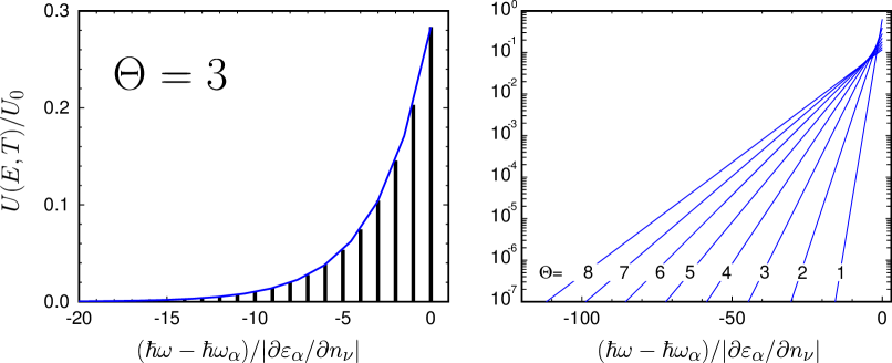
Figure 1: Envelope $U(E,T)$ of the absorption lineshapes $W^{\mathrm{dir,NP}}_{0\rightarrow\alpha}(\omega,T)$ as derived in (72). This function is meant to represents the exponential tail in the optical absorption spectrum just below the direct gap $\hbar\omega_{\alpha}$ of a solid. (a) Exponential decay of the absorption rate at the temperature $\Theta=3$, with $\Theta={k_{\rm B}T}/\hbar\Omega_{\nu}$ (blue curve). The vertical black lines represent the intensities of the Dirac delta functions in (71). (b) The absorption lineshapes plotted on a logarithmic scale at various temperatures, $\Theta=1,\dots,8$. We see that the lineshapes yield straight lines and radiate approximately from a common focus, as prescribed by the Urbach rule [43].

9 Unifying expressions for molecules and solids in a semiclassical approach

9.1 Motivation

In the previous sections we discussed two different viewpoints of the electron-phonon problem, the molecular picture and the solid-state picture. The reader will note that the expressions derived starting from the molecular picture are in general less complicated than their solid-state counterparts. For instance, the expression for the Herzberg-Teller rate (34) is far more compact than the solid-state partitioning of (59) into no-phonon, phonon-assisted, direct and indirect contributions. This behaviour can be attributed to the fact that solutions to the non-interacting Hamiltonian in the molecular picture (16) carry information about the excited state PES, while in the solid-state case this information must be recovered a posteriori through the perturbative term $\Delta H^{\mathrm{AH}}$ (24).

It is sensible therefore to ask whether the molecular picture can be applied to extended solid-state systems. The difficulty here is that calculating the $\alpha$-dependent nuclear wavefunctions through (6) requires knowledge of excited-state forces, which are highly nontrivial to calculate in extended systems [47]. An ideal compromise would be to find an approach which inherits the basic structure of the molecular picture but nonetheless avoids explicit evaluation of the $\alpha$-dependent nuclear wavefunctions. In this section we discuss such an approach.

9.2 Semiclassical approximation for electron-phonon renormalization and optical absorption

Here we consider the semiclassical approach originally proposed by Lax in Ref. [30] as an alternative to the Herzberg-Teller expression (34) in section 5.3. Its derivation proceeds by expressing the absorption rate appearing in (34) in the time domain,

$$W_{\alpha n\rightarrow\beta m}^{\mathrm{HT}}(\omega)=\frac{1}{\hbar}\int dte^{-i\omega t}W_{\alpha n\rightarrow\beta m}^{\mathrm{HT}}(t),$$ (76)

which gives:

$$W_{\alpha n\rightarrow\beta m}^{\mathrm{HT}}(t)=\frac{2\pi}{\hbar}\langle\chi_{\alpha n}|P_{\alpha\beta}^{R}|\chi_{\beta m}\rangle$$

$$\hskip 76.82234pt\times\langle\chi_{\beta m}|\exp\left(\frac{it}{\hbar}E_{\beta m}\right)P_{\beta\alpha}^{R}\exp\left(-\frac{it}{\hbar}E_{\alpha n}\right)|\chi_{\alpha n}\rangle.$$ (77)

As the nuclear wavefunctions are eigenstates of (6), we can replace the eigenvalues by the operators to find:

$$W_{\alpha n\rightarrow\beta m}^{\mathrm{HT}}(t) = \frac{2\pi}{\hbar}\langle\chi_{\alpha n}|P_{\alpha\beta}^{R}|\chi_{\beta m}\rangle$$

$$\times\!\langle\chi_{\beta m}|\exp\left[\frac{it}{\hbar}(T^{R}\!+U_{\beta}^{R})\right]\!P_{\beta\alpha}^{R}\!\exp\left[-\frac{it}{\hbar}(T^{R}\!+U_{\alpha}^{R})\right]|\chi_{\alpha n}\rangle.$$

The semiclassical approximation by Lax consists of neglecting all commutators involving the kinetic energy operator (e.g. $[T^{R},U_{\alpha}^{R}]$, $[T^{R},P_{\beta\alpha}^{R}]$ and so on). Using this simplification we can rewrite (LABEL:eq.timedomain) as follows:

$$W_{\alpha n\rightarrow\beta m}^{\mathrm{HT}}(t) \simeq \frac{2\pi}{\hbar}\langle\chi_{\alpha n}|P_{\alpha\beta}^{R}|\chi_{\beta m}\rangle\langle\chi_{\beta m}|\exp\left[\frac{it}{\hbar}(\varepsilon_{\beta}^{R}-\varepsilon_{\alpha}^{R})\right]\!P_{\beta\alpha}^{R}|\chi_{\alpha n}\rangle$$ (79)

where we used (4) and (5) to rewrite $U_{\beta}^{R}-U_{\alpha}^{R}=\varepsilon_{\beta}^{R}-\varepsilon_{\alpha}^{R}$. Now using (76) to return to the frequency domain, summing over all possible final vibrational states, and setting the initial electronic state to the ground state, we obtain the simple expression:

$$W^{\rm SC}_{0n\rightarrow\alpha}(\omega)=\langle\chi_{0n}|W^{R}_{0\rightarrow\alpha}(\omega)|\chi_{0n}\rangle,$$ (80)

with

$$W^{R}_{0\rightarrow\alpha}(\omega)=\frac{2\pi}{\hbar}|P_{\alpha 0}^{R}|^{2}\delta(\varepsilon_{\alpha}^{R}-\hbar\omega).$$ (81)

The expression (80) gives the optical absorption spectrum in terms of the average over the ground-state nuclear wavefunctions $\chi_{0n}(R)$ of the absorption spectra $W^{R}_{0\rightarrow\alpha}$ obtained for nuclei immobile in the configurations $R$. In (81) the electron-phonon interaction is taken into account via $\varepsilon_{\alpha}^{R}$, $P_{\alpha 0}^{R}$, and $\chi_{0n}(R)$, while the use of the relation $\sum_{m}|\chi_{\alpha m}\rangle\langle\chi_{\alpha m}|=1$ has removed the problematic $\alpha$-dependent nuclear wavefunctions. The approximation defined by (80) is referred to as “semiclassical” since it becomes exact in the limit where the nuclei are so heavy that the spectrum of the harmonic oscillator becomes continuous.

Performing the thermal average of (80) gives the temperature dependent semiclassical expression,

$$W^{\mathrm{SC}}_{0\rightarrow\alpha}(\omega,T)=\frac{1}{Z}{\sum}_{n}e^{-\frac{E_{0n}}{{k_{\rm B}T}}}\,W_{0n\rightarrow\alpha}^{\mathrm{SC}}(\omega).$$ (82)

This expression can be simplified further if we use Mehler’s formula [48]. In fact, after combining (81), (82), and (107) we obtain the compact result:

$$W^{\mathrm{SC}}(\omega,T)=\int{\prod}_{\nu}dx_{\nu}\frac{1}{\sqrt{2\pi\langle x_{\nu}^{2}\rangle_{T}}}\exp\left(-\frac{x_{\nu}^{2}}{2\langle x_{\nu}^{2}\rangle_{T}}\right)W^{R}_{0\rightarrow\alpha}(\omega),$$ (83)

with $R$ and $x_{\nu}$ related as in (94). This result has a simple intuitive interpretation: in the semiclassical approximation the temperature-dependent optical absorption spectrum is obtained by first calculating spectra for nuclei clamped in a variety of configurations $R$, and then averaging the spectra thus obtained using a gaussian importance function. The width of the importance function increases with the temperature as $\langle x_{\nu}^{2}\rangle_{T}=l_{\nu}^{2}\,[2n_{\rm B}(\Omega_{\nu},T)+1]$ (A).

An appealing aspect of the method proposed in this section is that it can be used without difficulty with any electronic structure package which can compute optical absorption spectra at fixed nuclei, without requiring a significant investment in software development. For example, in [32] we computed (80) for diamondoids using Importance Sampling Monte Carlo integration. Alternatively, Path-Integral Monte Carlo techniques can also be employed [49, 50].

9.3 Connection to the Herzberg-Teller effect in molecules and indirect absorption in solids

We stress that the approximation leading to (79) is purely heuristic, and the validity of the ensuing formulation should be assessed by comparing with the predictions of the complete theory. Here we limit ourselves to the analysis of the first frequency moment of the lineshape; a more comprehensive discussion can be found in Ref. [30]. By proceeding along the lines of section 5.4 we find the following expression relating the first frequency moment of the “exact” Herzberg-Teller lineshape, (34), and the “approximate” semiclassical lineshape, (80):

$$\langle\hbar\omega\rangle^{\rm HT}_{0n\rightarrow\alpha}=\langle\hbar\omega\rangle^{\rm SC}_{0n\rightarrow\alpha}+\frac{\langle\chi_{0n}|P_{0\alpha}^{R}[T^{R},P_{\alpha 0}^{R}]|\chi_{0n}\rangle}{\langle\chi_{0n}||P_{\alpha 0}^{R}|^{2}|\chi_{0n}\rangle}.$$ (84)

Analogous relations are found for higher frequency moments. The magnitude of the last term in (84) can be estimated from the linear expansion of $P_{0\alpha}^{R}$ as

$$\langle\hbar\omega\rangle^{\rm HT}_{0n\rightarrow\alpha}-\langle\hbar\omega\rangle^{\rm SC}_{0n\rightarrow\alpha}\sim\sum_{\nu}\hbar\Omega_{\nu}\left|\sum_{\gamma\neq\alpha}\frac{G^{\nu}_{\alpha\gamma}P_{\gamma 0}}{\varepsilon_{\alpha}-\varepsilon_{\gamma}}+\sum_{\gamma\neq 0}\frac{P_{\alpha\gamma}G^{\nu}_{\gamma 0}}{\varepsilon_{0}-\varepsilon_{\gamma}}\right|^{2}\frac{1}{|P_{0\alpha}|^{2}}.$$

This result indicates that the semiclassical lineshape is expected to capture very accurately the first moment of the complete Herzberg-Teller lineshape, since the error is a fraction $(G/E_{\rm g})^{2}$ of the characteristic vibrational energy, with $G$ a typical electron-phonon matrix element and $E_{\rm g}$ the fundamental gap.

In the case of solids it is possible to perform a similar analysis and show that the semiclassical approximation in (80) correctly captures the onset of direct and indirect absorption, both in terms of transition energies and oscillator strengths. As an example we consider here the oscillator strength for indirect absorption, which is obtained from (69) as:

$$\int d\omega\,W^{\rm ind,PA}_{0n\rightarrow\alpha}(\omega)=\frac{2\pi}{\hbar}\sum_{\nu}\left|\sum_{{\gamma}\neq\alpha}\frac{G^{\nu}_{\alpha{\gamma}}P_{{\gamma}0}}{\varepsilon_{\alpha}\!-\!\varepsilon_{\gamma}}+\sum_{{\gamma}\neq 0}\frac{P_{\alpha{\gamma}}G_{{\gamma}0}^{\nu}}{\varepsilon_{0}\!-\!\varepsilon_{\gamma}}\right|^{2}\!\!(2n_{\nu}+1)$$

$$\hskip 170.71652pt+{\mathcal{O}}(x_{\nu}^{4},3).\qquad\mbox{(a. a.)}$$ (85)

In order to reach this expression we used the fact that in the adiabatic approximation the vibrational energies are small with respect to the fundamental gap, $\hbar\Omega_{\nu}\ll E_{\rm g}$. The semiclassical counterpart of (9.3) is obtained from (80) and (81):

$$\int d\omega\,W^{\rm SC}_{0n\rightarrow\alpha}(\omega)=\frac{2\pi}{\hbar}\langle\chi_{0n}||P_{\alpha 0}^{R}|^{2}|\chi_{0n}\rangle.$$ (86)

By expanding the optical matrix element $P_{\alpha 0}^{R}$ in this expression about the equilibrium positions of the nuclei using (30) and (55), and setting $P_{0\alpha}=0$ (indirect process) we find:

$$P_{0\alpha}^{R}=\sum_{\nu}\left[\sum_{\gamma\neq 0}\frac{G^{\nu}_{0\gamma}P_{\gamma\alpha}}{\varepsilon_{0}-\varepsilon_{\gamma}}+\sum_{\gamma\neq\alpha}\frac{P_{0\gamma}G^{\nu}_{\gamma\alpha}}{\varepsilon_{\alpha}-\varepsilon_{\gamma}}\right](b_{\nu}^{\dagger}+b_{\nu})+{\mathcal{O}}(x_{\nu}^{2}).$$ (87)

The replacement of this expansion inside (86) yields, after using the standard algebra of ladder operators (A):

$$\int d\omega\,W^{\rm SC}_{0n\rightarrow\alpha}(\omega)=\int d\omega\,W^{\rm ind,PA}_{0n\rightarrow\alpha}(\omega)+{\mathcal{O}}(x_{\nu}^{4}).$$ (88)

This result indicates that the semiclassical approximation correctly captures the oscillator strength of indirect optical transitions in solids. A similar reasoning applies to direct transitions.

9.4 Advantages and shortcomings of the semiclassical approximation

The semiclassical approach defined by (82) carries the advantage of starting from the more accurate molecular non-interacting Hamiltonian without needing information about the $\alpha$-dependent nuclear wavefunction. As such, it provides a unified framework for studying solids and molecules using exactly the same formalism and the same computational techniques. This aspect is especially important given the large volume of research activity in the areas of nanoscience and nanotechnology, where one is often confronted with heterogeneous systems, e.g. molecular adsorbates on surfaces.

The main shortcoming of the semiclassical approach in molecules is that the characteristic Franck-Condon structure consisting of distinct vibronic peaks is completely lost. In fact, as the numerical tests of Ref. [51] demonstrate, the neglect of the commutators in (LABEL:eq.timedomain) destroys precisely the quantisation of the vibrational energy levels. In practice the semiclassical approximation in molecules is very useful for calculating the envelope of the absorption profile, without resolving individual vibronic transitions. Additionally the semiclassical approximation is expected to improve as the size of the molecule increases. This is clearly demonstrated in our earlier work on diamondoids [32], where we showed that in the case of triamantane (C₁₈H₂₄) the semiclassical approach yields excellent agreement with experiment.

Apart from the practical advantage of (82) only relying on the nuclear wavefunctions $\chi_{0n}$ in the electronic ground state, an additional strength is found by noting that the approach requires neither the harmonic approximation nor the adiabatic approximation to be satisfied by the excited states. This observation is supported by empirical evidence: the model calculations of Ref. [52] demonstrate that the semiclassical expression can capture non-adiabatic Jahn-Teller effects; in addition, our calculations of the optical spectra of adamantane within the semiclassical approach [32] are in excellent agreement with experiment, even though this molecule has a triply degenerate highest-occupied molecular orbital and undergoes a Jahn-Teller splitting upon excitation [53] (B.2).

In summary the semiclassical approach seems to offer a useful compromise between computational simplicity, accuracy, and broad applicability to the widest range of systems. First-principles calculations will be needed to carry out a systematic assessment of the performance of this method in reproducing experimental spectra. In the following section we demonstrate the application of (82) to the calculation of the optical absorption spectrum of bulk silicon.

10 The semiclassical approximation applied to bulk silicon

10.1 Introduction

In this section we apply some of the expressions derived above to the prototypical indirect gap semiconductor, bulk silicon. As noted in the introduction to this manuscript, there has been phenomenal progress in the developments of electronic structure methods for dealing with the many-electron problem [22]. Here we shall work at the level of the local density approximation to density-functional theory. Although such calculations generally fail to obtain quantitative agreement with experimental observations (most famously underestimating the band gap), qualitative features can be reproduced. As discussed in section 11, the calculation of electron-phonon renormalization and phonon-assisted optical absorption using more complicated electronic structure methods is an important subject for future research.

10.2 Computational approach

Here we describe the technical details of our calculations. The reader interested in results may choose to skip to section 10.3.

10.2.1 Electronic structure

We calculate the energy-level renormalization and optical absorption spectra using (10) and (82). We replace the electronic excitation energies $\varepsilon_{\alpha}$ appearing in these equations with Kohn-Sham eigenvalues obtained within the local-density approximation to DFT [19, 20]. Similarly the many-body matrix elements $P_{\beta\alpha}^{R}$ (35) are replaced by those taken between single-particle Kohn-Sham wavefunctions.

10.2.2 Energy-level renormalization

We evaluate the energy-level renormalization in two ways. In the first case, we obtain the electron-phonon coupling coefficients $\partial\varepsilon_{\alpha}/\partial n_{\nu}$ by averaging the energies $\varepsilon_{\alpha}^{R}$ calculated after displacing the nuclei by amplitudes $\pm\sqrt{(}\hbar/M_{p}\Omega_{\nu})$ along a phonon mode $\nu$, which isolates the quadratic term in the expansion (11) [35]. Substituting the calculated coefficients into (12) yields the temperature-dependent energy $\langle\varepsilon_{\alpha}\rangle_{T}$. Alternatively, we can obtain $\langle\varepsilon_{\alpha}\rangle_{T}$ directly from the analogue of (83), i.e.:

$$\langle\varepsilon_{\alpha}\rangle_{T}=\int{\prod}_{\nu}dx_{\nu}\frac{1}{\sqrt{2\pi\langle x_{\nu}^{2}\rangle_{T}}}\exp\left(-\frac{x_{\nu}^{2}}{2\langle x_{\nu}^{2}\rangle_{T}}\right)\varepsilon_{\alpha}^{R}.$$ (89)

Calculating $\langle\varepsilon_{\alpha}\rangle_{T}$ in this way allows us to assess the impact of neglecting the $x_{\nu}^{4}$ terms in (12). In the case that eigenvalues are degenerate at the equilibrium structure, we evaluate $\langle\varepsilon_{\alpha}\rangle_{T}$ as a trace (B.2).

10.2.3 Absorption spectra

In order to compare our absorption spectrum to experiment, we construct the absorption coefficient $\kappa$ as

$$\kappa(\omega,T)=\frac{\omega}{c}\frac{\epsilon_{2}(\omega,T)}{n^{r}},$$ (90)

where $n^{r}$ is the refractive index. Here for simplicity we neglect the frequency and temperature dependence of the refractive index, and use the experimental value $n^{r}=3.4$ [54]. The temperature-dependent imaginary part of the dielectric function $\epsilon_{2}(\omega,T)$ is found by noting that, for clamped ions $\epsilon^{R}_{2}(\omega)\propto\ \sum_{\alpha}1/\omega\ W^{R}_{0\rightarrow\alpha}(\omega)$; therefore in the semiclassical picture (82) we obtain

$$\epsilon_{2}(\omega,T)=\int{\prod}_{\nu}dx_{\nu}\frac{1}{\sqrt{2\pi\langle x_{\nu}^{2}\rangle_{T}}}\exp\left(-\frac{x_{\nu}^{2}}{2\langle x_{\nu}^{2}\rangle_{T}}\right)\epsilon_{2}^{R}(\omega)$$ (91)

In practice we use the momentum representation of the matrix elements to evaluate $\epsilon^{R}_{2}(\omega)$, and neglect the commutator term arising from the nonlocal part of the pseudopotential [55]. We replace the $\delta$-functions which appear in $\epsilon^{R}_{2}(\omega)$ with Gaussians of width 0.2 eV for the spectrum obtained with fixed ions and 0.02 eV for the semiclassical calculation. Finally, in order to account to the band gap problem, we impose a rigid scissor shift of 0.7 eV to the energies of the unoccupied Kohn-Sham states, obtained as the difference between DFT and $GW$ calculations in Ref. [56].

10.2.4 Sampling method

In both (89) and (91) we must evaluate an integral over all nuclear displacements. In a previous work [32] we recast the integral as a sum over a large sample of nuclear geometries, generated such that the phonon displacements $x_{\nu}$ were distributed according to the Gaussian factor $\exp\left(-x_{\nu}^{2}/2\langle x_{\nu}^{2}\rangle_{T}\right)$. Here we repeat that general approach, but employ the method described in Ref. [57] to generate the sample. This method replaces uniformly-distributed random numbers in the generation algorithm with a low-discrepancy (Sobol) sequence, which greatly improves the convergence properties in higher-dimensional systems [58]. We used sample sizes of 200 steps to compute both the energy-level renormalization and optical spectrum. We tested the convergence of the former by increasing the sample size to 500 steps, and found the calculated corrections to change by less than 2 meV.

10.2.5 Computational details

Electronic structure calculations were performed within the local-density approximation to DFT, using plane-wave basis sets and periodic boundary conditions implemented in the Quantum ESPRESSO distribution [59]. We used a norm-conserving pseudopotential [60] to descibe the Si ion and expanded the electronic wavefunctions in reciprocal space up to an energy cutoff of 35 Ry. For the calculation of the energy-level renormalization we used a $4\times 4\times 4$ supercell and sampled the electrons at the $\Gamma$-point, while for the optical spectrum we used a $2\times 2\times 2$ supercell with an $8\times 8\times 8$ Brillouin Zone sampling of the electrons (i.e. an effective electronic sampling of $16\times 16\times 16$). The equilibrium structures were calculated by varying the lattice parameter $a$ until the force on each atom was less than 0.03 eV/Å and the pressure less than 0.5 kbar, yielding values of 5.41 and 5.31 Å for the $4\times 4\times 4$/$2\times 2\times 2$ supercells. The phonon modes were determined by displacing each ion in the primitive cell by 0.005 Å, obtaining the forces, then using the translational symmetry and appropriate sum rules [61] to construct the dynamical matrix of the supercell.

10.3 Energy-level renormalization

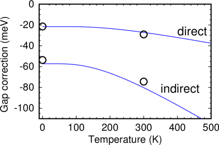
Figure 2: Calculated temperature dependent corrections to the direct and indirect gaps of silicon. The blue lines were obtained over the entire temperature range from (12), while the circles were calculated at specific temperatures (0 K and 300 K) using (89).

Silicon is an indirect gap semiconductor, with the valence band maximum located at the $\Gamma$-point and the conduction band minimum located close to the $X$-point. With the ions frozen in their equilibrium positions we find a value of 2.55 eV for the direct gap at $\Gamma$ and a value of 0.62 eV for the indirect $X$-$\Gamma$ gap. We introduce the temperature-dependent corrections to these gaps as $(\langle\varepsilon_{\alpha}\rangle_{T}-\langle\varepsilon_{\beta}\rangle_{T})-(\varepsilon_{\alpha}-\varepsilon_{\beta})$, where $\beta$ refers to the occupied state at the $\Gamma$ point and $\alpha$ refers to the unoccupied states either at the $\Gamma$ point (direct gap) or $X$ point (indirect gap).

The values obtained for the gap corrections over the entire temperature range using (12) are shown as the blue lines in Fig. 2. We also plot as circles the corrections obtained at 0 K and 300 K using (89).

In general, we see that the quantum motion of the nuclei acts to close the band gap, albeit only by a small amount. Using the quadratic expansion of (12), we obtain zero-point corrections of -22 meV and -57 meV to the direct and indirect gaps. The zero-point correction obtained for the indirect gap is close to the value of -52 meV found in recent calculations [39]. At 300 K the magnitudes of these corrections increase slightly, to 27 and 80 meV for the direct and indirect gaps respectively.

Using (89), we calculate corrections of -21 and -54 meV to the direct and indirect gaps at 0 K, and -29 and -74 meV at 300 K. Within the error expected from our sampling procedure, these values are equal to those obtained with (12). Thus the neglect of the ${\mathcal{O}}(x_{\nu}^{4})$ in the latter approach is justified in this case.

10.4 Phonon assisted absorption

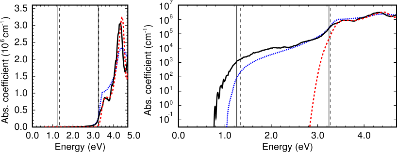
Figure 3: The absorption coefficient of bulk silicon, calculated with the ions fixed in their equilibrium positions (red dashed lines) and with the semiclassical expression (91) at 300 K (black line), compared to the experimental measurements of Ref. [54] (blue dotted line). The same data are shown on linear (left) and logarithmic (right) scales. The vertical lines indicate the calculated band gaps (including scissor correction), both with nuclei fixed in their equilibrium positions (dashed) and after including temperature renormalization at 300 K, from Fig. 2 (solid).

We now turn to the optical absorption spectrum. In Fig. 3 we plot the absorption coefficient obtained for the Si ions fixed in their equilibrium positions (red line), and compare to the experimental measurements at 300 K reported in Ref. [54] (blue line). The theoretical fixed-ion spectrum displays no absorption until the direct onset at 3.3 eV, while in experiment indirect transitions are observed above the threshold of 1.1 eV.

When we evaluate the semiclassical expression (91) at 300 K (black line) we find that the theoretical spectrum correctly displays absorption below the direct gap. The absorption coefficient slowly increases in magnitude over the region 1.1–3.3 eV, before a sharp increase above the direct gap threshold.

The semiclassical lineshape obtained here is not in perfect agreement with experiment. We assign the discrepancy to our use of a small supercell, equivalent to a $2\times 2\times 2$ $\vec{q}$-point sampling (by contrast the calculations of Ref. [10] used the Wannier interpolation scheme of Ref. [62] to obtain extremely fine $\vec{q}$ grids, up to $40\times 40\times 40$). The $2\times 2\times 2$ sampling is sufficient for us to at least observe the indirect $X-\Gamma$ transition, but it is likely that the inclusion of more phonon modes will redistribute the spectral weight in this energy region. Investigating the convergence of the spectrum with increasing supercell size is an important topic for future study.

Apart from this discrepancy, our calculated spectrum in Fig. 3 illustrates that the semiclassical approximation discussed in section 9 captures phonon-assisted indirect optical absorption in solids. Furthermore this simple approach automatically incorporates the temperature dependence of the energy levels and their zero-point renormalization, shown by the vertical lines in Fig. 3.

11 Choice of the electronic Hamiltonian

Throughout this manuscript we employed a formalism based on the many-body electronic Hamiltonian $H_{e}^{R}(r)$, wavefunctions $\Psi_{\alpha}^{R}(r)$, and eigenstates $E_{\alpha}^{R}$, see (2) and (3). In practical calculations these quantities need to be replaced with appropriate approximations, for example the Hartree-Fock method or the Kohn-Sham formulation of DFT [20, 63].

If we consider Kohn-Sham DFT [20], then the electronic Hamiltonian at fixed nuclei is replaced by the self-consistent Kohn-Sham Hamiltonian, and the many-body wavefunctions are replaced by Slater determinants of Kohn-Sham single-particle states, as we have done in section 10. After these substitutions all the formalism presented in this work remains essentially unchanged. For example, if the determinants $|\Psi_{\alpha}\rangle$ and $|\Psi_{\beta}\rangle$ differ only in the occupations of the single-particle states $\psi_{\alpha}$ and $\psi_{\beta}$, then the many-body electron-phonon matrix elements $G_{\alpha\beta}^{R}$ introduced in (54) need to be replaced by matrix elements of of the self-consistent Kohn-Sham potential taken between these Kohn-Sham states, $g_{\alpha\beta}^{\nu}=\langle\psi_{\alpha}({\bf r})|\Delta_{\nu}V_{\rm SCF}^{R}({\bf r})|\psi_{\beta}({\bf r})\rangle$ (with $\Delta_{\nu}=l_{\nu}\partial/\partial x_{\nu}$). Similarly, the quadratic electron-phonon couplings $\partial\varepsilon_{\alpha}/\partial n_{\nu}$ in (13) need to be evaluated using differences in Kohn-Sham eigenvalues for the excitation energies. Calculations of electron-phonon renormalization based on single-particle Hamiltonians (either empirical or DFT) are abundant in the literature [11, 13, 35, 36, 14, 37, 31, 32], therefore it is expected that the formalism presented here will find immediate application in such calculations, as demonstrated in the previous section.

In more sophisticated approaches it should be possible to describe excited states using the solutions of the two-particle Bethe-Salpeter equation [22]: $|\Psi_{\alpha}\rangle=\sum_{cv}A_{cv}^{\alpha}a_{c}a^{\dagger}_{v}|\Psi_{0}\rangle$, with $a_{c}$ and $a_{v}^{\dagger}$ the operators for creating an electron and a hole in the single-particle states $\psi_{c}$ and $\psi_{v}$, respectively, and $A_{cv}^{\alpha}$ the Bethe-Salpeter eigenvector. In this case the many-body electron-phonon matrix element in (54) would incorporate both the eigenvectors $A_{cv}^{\alpha}$ and the Kohn-Sham electron-phonon matrix elements $g_{cv}^{\nu}$. This alternative approach could be used to investigate exciton-phonon interactions, provided practical approximations for the variation of the Bethe-Salpeter Kernel with the nuclear positions can be found, for example along the lines of Ref. [47].

The large flexibility afforded by the present formulation stems precisely from the choice of introducing nuclear PES using (4), without making any assumptions on the underlying electronic Hamiltonian at fixed nuclei.

12 Summary and conclusions

Table 1: Summary of key results obtained in this work for quick reference. The first two sets apply to solids and molecules, respectively, and reflect the different choices of the non-interacting Hamiltonians. The last set provides a unified description of electron-phonon effects in the optical spectra of solids and molecules, irrespective of system size.

	Solids
	Description	Equation
	Allen-Heine theory	(12)
	Zero-point renormalization	(45)
	No-phonon direct absorption	(62)
	Phonon-assisted direct absorption	(67)
	Phonon-assisted indirect absorption	(70)
	Exponential Urbach tail	(72)
	Molecules
	Description	Equation
	Born-Huang expansion	(31)
	Franck-Condon theory	(37)
	Herzberg-Teller theory	(34)
	Molecules and Solids
	Description	Equation
	Semiclassical approximation to optical absorption	(80)
	Temperature-dependent absorption using Mehler’s formula	(83)

In this work we presented an attempt to place the theories of electron-phonon effects in the optical spectra of solids and molecules within a common framework.

We showed that the discussion of these phenomena in the quantum chemistry literature and in the solid-state physics literature differ by the choice of the underlying non-interacting electron-phonon Hamiltonian: in the case of molecules (which by extension emcompasses the cases of point defects and Frenkel excitons in solids) the nuclei experience a different potential energy surface for each electronic excitation, whilst in the case of solids the nuclear dynamics is described by considering only the PES generated by the electrons in their ground state. This subtle difference can be identified as the origin of the widely different approaches and methods developed for studying electron-phonon effects in chemistry and in physics.

Concentrating on molecules, we showed how well-established conceptual models of electron-phonon effects in molecules, such as the Franck-Condon theory, the Born-Huang expansion, and the Herzberg-Teller effect, can all be obtained by straightforward low-order time-independent perturbation theory.

Along similar lines, we were able to derive the standard expression for indirect optical absorption in solids using time-independent perturbation theory. In this case our analysis revealed a number of subtle effects which have gone largely unnoticed in the literature, for example we identified phonon-assisted optical absorption in direct band gap materials.

The present work also allowed us to identify an exponential tail in the optical absorption edge, which we tentatively assigned to the famous Urbach tail. To the best of our knowledge, this is the first time that an exponential edge emerges from a first-principles theory, while earlier proposals invariably used phenomenological models.

We analyzed the formal basis of the Allen-Heine theory of temperature-dependent band structures. In this case we showed that the off-diagonal couplings between nuclear wavefunctions yield a correction to the zero-point renormalization not usually considered in first-principles calculations.

Finally, we considered the semiclassical approach proposed in Ref. [30] for molecules as an avenue to calculating optical absorption across the length scales. In particular we pointed out that the resulting expression avoids the difficulties associated with nuclear wavefunctions corresponding to excited-state potential energy surfaces, and that it applies generally also to the case of solids. We demonstrated an application of this expression by calculating the phonon-assisted optical absorption spectrum of bulk silicon. We provide a quick reference to our main results in Table 1.

One important aspect of our theory is that the electron-phonon renormalization and the phonon-assisted optical absorption are described on the same footing. This strategy leads to a consistent theory of temperature-dependent optical absorption, and avoids the ambiguity that arises when trying to merge the theory of indirect absorption with that of temperature-dependent band structures.

In this work an effort was made to develop the theory by relying on a minimal set of approximations. In order to keep the discussion accessible to the broadest audience we purposely refrained from making specific assumptions, e.g. the form of the electronic Hamiltonian at fixed nuclei or the translational invariance and the reciprocal space formalism for solids. This choice should make it easier to tailor the present theory to specific applications, and work is currently in process to assess the performance of the formalism within the context of first-principles calculations.

It is hoped that the theory developed here will help clarifying the links between the many different approaches to the electron-phonon problem, and will serve as a general and well defined conceptual framework for future first-principles calculations of optical spectra.

Appendix A Normal modes of vibrations and ladder operators

In order to make the manuscript self-contained we review the basic concepts and quantities needed to describe the ground-state nuclear PES, $U^{R}_{0}$, in the harmonic approximation [17]. By expanding $U^{R}_{0}$ in powers of the nuclear displacements from their equilibrium geometry $R_{0}$ and retaining terms up to second order (harmonic approximation) we have:

$$U^{R}_{0}=U^{R_{0}}_{0}+\frac{1}{2}\sum_{I\kappa,J\lambda}\frac{\partial^{2}U^{R}_{0}}{\partial R_{I\kappa}R_{J\lambda}}u_{I\kappa}u_{J\lambda},$$ (92)

where $u_{I\kappa}$ denotes the displacement from equilibrium of the $I$-th nucleus along the Cartesian direction $\kappa$, and similary for $u_{J\lambda}$. From this expression the dynamical matrix is introduced as:

$$D_{I\kappa,J\lambda}=\sqrt{\frac{1}{M_{I}M_{J}}}\left.\frac{\partial^{2}U^{R}_{0}}{\partial R_{I\kappa}R_{J\lambda}}\right|_{R_{0}},$$ (93)

where $M_{I}$ and $M_{J}$ are the nuclear masses. Let us denote by $e^{\nu}_{I\kappa}$ the eigenvector of this matrix for the eigenvalue $\Omega_{\nu}^{2}$. We can perform the transformation to normal mode coordinates $x_{\nu}$ as follows:

$$u_{I\kappa}=\sqrt{\frac{M_{P}}{M_{I}}}\sum_{\nu}e^{\nu}_{I\kappa}x_{\nu},$$ (94)

where $M_{P}$ is a reference mass (usually the mass of a proton). In normal mode coordinates the PES becomes:

$$U_{0}^{R}=U^{R_{0}}_{0}+{\sum}_{\nu}\frac{1}{2}M_{P}\Omega_{\nu}^{2}x_{\nu}^{2}.$$ (95)

By applying the same coordinate transformation to the kinetic energy we can rewrite (7) as:

$$\sum_{\nu}\left[-\frac{\hbar^{2}}{2M_{P}}\frac{\partial^{2}}{\partial x_{\nu}^{2}}+\frac{1}{2}M_{P}\Omega_{\nu}^{2}x_{\nu}^{2}\right]\chi_{0n}=\left[E_{0n}-U^{R_{0}}_{0}\right]\chi_{0n}.$$ (96)

The solution of this equation is obtained as a product of independent quantum harmonic oscillators, $\chi_{0n}={\prod}_{\nu}\phi_{n_{\nu}}(x_{\nu})$, with:

$$\phi_{n_{\nu}}(x_{\nu})=\frac{(2\pi l_{\nu}^{2})^{-1/4}}{\sqrt{2^{n_{\nu}}n_{\nu}!}}\exp\left(-\frac{x_{\nu}^{2}}{4l_{\nu}^{2}}\right)H_{n_{\nu}}\left(\frac{x_{\nu}}{\sqrt{2}l_{\nu}}\right),$$ (97)

and energy $E_{0n_{\nu}}=\hbar\Omega_{\nu}(1/2+n_{\nu})$. In this equation $H_{n_{\nu}}(x)$ is the Hermite polynomial of order $n_{\nu}$ and $l_{\nu}$ is defined as in (14). The set of quantum numbers $n_{1},n_{2},\dots$ defines the composite index $n$ in the wavefunction $\chi_{0n}$, and identify the occupations of each vibrational quantum state. It is customary to indroduce the ladder operators $b_{\nu}^{\dagger}$ and $b_{\nu}$ such that:

$$b^{\dagger}_{\nu}|\phi_{n_{\nu}}\rangle=\sqrt{n_{\nu}+1}|\phi_{n_{\nu}+1}\rangle,\qquad b_{\nu}|\phi_{n_{\nu}}\rangle=\sqrt{n_{\nu}}|\phi_{n_{\nu}-1}\rangle.$$ (98)

These operators have the following useful properties which are used repeatedly throughout the manuscript:

$$[b_{\nu},b^{\dagger}_{\mu}]=\delta_{\nu\mu},$$ (99)

$$b^{\dagger}_{\nu}b_{\nu}|\phi_{n_{\nu}}\rangle=n_{\nu}|\phi_{n_{\nu}}\rangle,$$ (100)

$$x_{\nu}=l_{\nu}(b^{\dagger}_{\nu}+b_{\nu}),$$ (101)

$$x_{\nu}^{2}=l_{\nu}^{2}(b^{\dagger}_{\nu}b^{\dagger}_{\nu}+b_{\nu}b_{\nu}+2b^{\dagger}_{\nu}b_{\nu}+1).$$ (102)

In addition the kinetic energy operator can be rewritten in terms of ladder operators as:

$$T^{R}=-\frac{1}{4}\sum_{\nu}\hbar\Omega_{\nu}(b^{\dagger}_{\nu}-b_{\nu})^{2}.$$ (103)

Using (98) and (102) the expectation value of the square displacement is obtained as:

$$\langle\phi_{n_{\nu}}|x_{\nu}^{2}|\phi_{n_{\nu}}\rangle=l_{\nu}^{2}(2n_{\nu}+1),$$ (104)

and the corresponding thermal average is given by:

$$\langle x^{2}_{\nu}\rangle_{T}=\frac{1}{Z}{\sum}_{n_{\nu}=0}^{\infty}\exp\left[-\frac{E_{0n_{\nu}}}{{k_{\rm B}T}}\right]l_{\nu}^{2}(2n_{\nu}+1)=l_{\nu}^{2}[2n_{B}(\Omega_{\nu},T)+1],$$ (105)

with $Z={\sum}_{n_{\nu}=0}^{\infty}\exp(-E_{0n_{\nu}}/{k_{\rm B}T})$ being the canonical partition function and $n_{\rm B}$ the Bose-Einstein distribution. The total energy of the state $E_{0n}$ is:

$$E_{0n}=U^{R_{0}}_{0}+{\sum}_{\nu}\hbar\Omega_{\nu}\left[\frac{1}{2}+n_{\nu}\right].$$ (106)

The eigenstates of the quantum harmonic oscillator have the following useful property:

$$\frac{1}{Z}{\sum}_{n_{\nu}=0}^{\infty}e^{-\frac{E_{0n_{\nu}}}{{k_{\rm B}T}}}|\phi_{n_{\nu}}(x_{\nu})|^{2}=\frac{1}{\sqrt{2\pi\langle x^{2}_{\nu}\rangle_{T}}}\exp\left[-\frac{x^{2}}{2\langle x^{2}_{\nu}\rangle_{T}}\right],$$ (107)

with $\langle x^{2}_{\nu}\rangle_{T}$ given by (104). This result derives directly from (97) and Mehler’s formula [48]:

$$\sum_{n=0}^{\infty}\frac{\exp\left[-(x^{2}+y^{2})/2\right]}{2^{n}n!\sqrt{\pi}}t^{n}H_{n}(x)H_{n}(y)=$$

$$\qquad\qquad\frac{1}{\sqrt{\pi(1-t^{2})}}\exp\left[\frac{4xyt-(x^{2}+y^{2})(1+t^{2})}{2(1-t^{2})}\right],$$ (108)

with $x$, $y$, and $t$ real numbers.

Appendix B Perturbative expansions

B.1 General formulas

All the results presented in this work are based on standard time-independent nondegenerate perturbation theory [18]. For ease of reference we report here the key equations employed throughout the manuscript. The eigenstates of total Hamiltonian of the joint electron-nuclear system, ${\mathcal{H}}$ in (1), are denoted by $|\alpha n^{\rm e}\rangle$, with the superscript standing for “exact”. The corresponding energy is denoted as $E_{\alpha n}^{\rm e}$: ${\mathcal{H}}|\alpha n^{\rm e}\rangle=E_{\alpha n}^{\rm e}|\alpha n^{\rm e}\rangle$. We express the total Hamiltonian as the sum of a “non-interacting” Hamiltonian, $H_{0}$, and a perturbation, $\Delta H$, so that the non-interacting eigenstates and eigenvalues are given by: $H_{0}|\alpha n\rangle=E_{\alpha n}|\alpha n\rangle$. The second-order perturbative expansion of the energy $E_{\alpha n}^{\rm e}$ is given by:

$$E_{\alpha n}^{\rm e}=E_{\alpha n}+\langle\alpha n|\Delta H|\alpha n\rangle+{\sum_{\beta m}}^{\prime}\frac{|\langle\beta m|\Delta H|\alpha n\rangle|^{2}}{E_{\alpha n}-E_{\beta m}}+{\mathcal{O}}(3),$$ (109)

where the prime on the summation is to exclude the term with $\alpha=\beta$ and $n=m$. The first-order expansion of the eigenstate $|\alpha n^{\rm e}\rangle$ is:

$$|\alpha n^{\rm e}\rangle = |\alpha n\rangle+{\sum_{\beta m}}^{\prime}\frac{\langle\beta m|\Delta H|\alpha n\rangle}{E_{\alpha n}-E_{\beta m}}|\beta m\rangle+{\mathcal{O}}(2).$$ (110)

In both expressions the notation ${\mathcal{O}}(n)$ stands to indicate that the neglected terms are proportional to $\langle\beta m|\Delta H|\alpha n\rangle^{n}$.

The choice of the non-interacting Hamiltonians in section 4 guarantees that the use of perturbation theory is legitimate. In fact, if we consider for instance the case of solids, the size of the first order correction to the energy in (109) is of the order of the ratio between a characteristic phonon energy and the band gap, $\hbar\Omega_{\nu}/E_{\rm g}$ [38].

B.2 Degeneracies in the electronic spectrum

In this work we considered exclusively the case of non-degenerate perturbation theory. In the case that electronic states calculated for nuclei in their equilibrium positions $R_{0}$ are degenerate, i.e. $E_{\alpha}=E_{\beta}$, there exists an ambiguity in the perturbation expansion. This is best seen by considering (18), which shows that the energy denominator $E_{\alpha}-E_{\beta}$ yields a singularity. In this case it is necessary to repeat the entire set of derivations presented in this work using degenerate perturbation theory [18]. Following the prescription of degenerate perturbation theory, we would need to set the gauge of the wavefunctions in the degenerate subspace by diagonalizing the perturbation $\Delta H$ in the same subspace.

The treatment of electronic degeneracies does not pose any problems in the semiclassical approach described in section 9, since the degeneracy is traced out in the evaluation of the optical absorption spectra. This is easily understood by noting that the key equation (80) does not contain any energy denominators. The situation is more complex in the solid-state picture and in the molecular picture described in sections 4.1 and 4.2, respectively. In fact in the molecular case electronic degeneracies correspond to crossings of potential energy surfaces. These crossings are responsible for non-adiabatic couplings and have been the subject of numerous investigations in the quantum chemistry literature [27, 52]. In the case of solids the electronic degeneracies can be addressed by modifying the definition of the perturbative correction in (24) in such a way as to treat the non-degenerate and the degenerate parts separately.

B.3 Order of perturbative corrections

Throughout the manuscript we indicated the order of the perturbative expansion using alternatively the notation ${\mathcal{O}}(n)$ or ${\mathcal{O}}(x_{\nu}^{n})$. This distinction is important in the study of electron-phonon interactions, as already pointed out in Ref. [4].

In order to make this point clear we consider the matrix elements for optical transitions in solids, $\langle\beta m^{\rm e,s}|\Delta|\alpha n^{\rm e,s}\rangle$. In (49) this matrix element is expanded up to order ${\mathcal{O}}(2)$ in the perturbation $H_{e}^{R}-H_{e}^{R_{0}}$. However, the terms $\varepsilon_{\alpha}^{R}$ and $V_{\alpha\beta}^{R}$ appearing in (51)–(53) can be expanded further in terms of nuclear displacements to arbitrary order. For example, these terms are given in (55)–(56) up to an error of order ${\mathcal{O}}(x_{\nu}^{2})$.

More generally, an expansion to order ${\mathcal{O}}(n)$ always implies that the expression is also correct up to errors of order at least ${\mathcal{O}}(x_{\nu}^{n})$, but the reverse is not true in general. For this reason it is important to always follow the sequence of expanding first in terms of the Hamiltonian perturbation $\Delta H$, and then in terms of the nuclear displacements.

While this simple rule appears obvious, a considerable amount of debate in the literature was generated precisely by confusion on this point, most notably the link between the Fan and Debye-Waller corrections to the band structures of solids [4].

References

References

- [1] R M Martin. Electronic Structure: Basic Theory and Practical Methods. Cambridge: Cambridge University Press, 2004.
- [2] R O Jones and O Gunnarsson. The density functional formalism, its applications and prospects. Rev. Mod. Phys., 61:689, 1989.
- [3] S G Louie and M L Cohen, editors. Conceptual Foundations of Materials: A standard model for ground- and excited-state properties. Amsterdam: Elsevier, 2006.
- [4] P B Allen and V Heine. Theory of the temperature dependence of electronic band structures. J. Phys. C: Solid State Phys, 9:2305, 1976.
- [5] F Bassani and G Pastori Parravicini. Electronic States and Optical Transition in Solids. Oxford: Pergamon Press, 1975.
- [6] F Urbach. The long-wavelength edge of photographic sensitivity and of the electronic absorption of solids. Phys. Rev., 92:1324, 1953.
- [7] I C Cheeseman. The structure of the long wave absorption edge of insulating crystals. Proc. Phys. Soc. A, 65:25, 1952.
- [8] L H Hall, J Bardeen, and F J Blatt. Infrared absorption spectrum of Germanium. Phys. Rev., 95:559, 1954.
- [9] H Y Fan. Infra-red absorption in semiconductors. Rep. Prog. Phys., 19:107, 1956.
- [10] J Noffsinger, E Kioupakis, C G Van de Walle, S G Louie, and M L Cohen. Phonon-assisted optical absorption in silicon from first principles. Phys. Rev. Lett., 108:167402, 2012.
- [11] F Giustino, S G Louie, and M L Cohen. Electron-phonon renormalization of the direct band gap of diamond. Phys. Rev. Lett., 105:265501, 2010.
- [12] E Cannuccia and A Marini. Effect of the quantum zero-point atomic motion on the optical and electronic properties of diamond and trans-polyacetylene. Phys. Rev. Lett., 107:255501, 2011.
- [13] A Marini. Ab initio finite-temperature excitons. Phys. Rev. Lett., 101:106405, 2008.
- [14] X Gonze, P Boulanger, and M Côté. Theoretical approaches to the temperature and zero-point motion effects on the electronic band structure. Ann. Phys. (Berlin), 523:168, 2011.
- [15] F Santoro, A Lami, R Improta, J Bloino, and V Barone. Effective method for the computation of optical spectra of large molecules at finite temperature including the Duschinsky and Herzberg-Teller effect: The band of porphyrin as a case study. J. Chem. Phys., 128(22):224311, 2008.
- [16] P W Atkins and R S Friedman. Molecular Quantum Mechanics. Oxford: Oxford University Press, 2010.
- [17] J C Inkson. Many-Body Theory of Solids. New York: Plenum Press, 1983.
- [18] J J Sakurai. Modern Quantum Mechanics. Addison-Wesley, 1994.
- [19] P Hohenberg and W Kohn. Inhomogeneous electron gas. Phys. Rev., 136:B864, 1964.
- [20] W Kohn and L J Sham. Self-consistent equations including exchange and correlation effects. Phys. Rev., 140:A1133, 1965.
- [21] E Runge and E K U Gross. Density-functional theory for time-dependent systems. Phys. Rev. Lett., 52:997, 1984.
- [22] G Onida, L Reining, and A Rubio. Electronic excitations: density-functional versus many-body Green’s-function approaches. Rev. Mod. Phys., 74:601, 2002.
- [23] G Onida, L Reining, R W Godby, R Del Sole, and W Andreoni. Ab Initio calculations of the quasiparticle and absorption spectra of clusters: The sodium tetramer. Phys. Rev. Lett., 75:818, 1995.
- [24] M Rohlfing and S G Louie. Electron-hole excitations in semiconductors and insulators. Phys. Rev. Lett., 81:2312, 1998.
- [25] I Shavitt and R J Bartlett. Many-Body Methods in Chemistry and Physics: MBPT and Coupled-Cluster Theory. Cambridge: Cambridge University Press, 2009.
- [26] M E Casida. Time-dependent density functional theory for molecules. In D E Chong, editor, Recent Advances in Density Functional Methods, page 155. Singapore: World Scientific, 1995.
- [27] W Domcke and D R Yarkony. Role of conical intersections in molecular spectroscopy and photoinduced chemical dynamics. Annu. Rev. Phys. Chem., 63:325, 2012.
- [28] S Baroni, S de Gironcoli, A Dal Corso, and P Giannozzi. Phonons and related crystal properties from density-functional perturbation theory. Rev. Mod. Phys., 73:515, 2001.
- [29] B Monserrat, N D Drummond, and R J Needs. Anharmonic vibrational properties in periodic systems: energy, electron-phonon coupling, and stress. Phys. Rev. B, 87:144302, 2013.
- [30] M Lax. The Franck-Condon principle and its application to crystals. J. Chem. Phys., 20:1752, 1952.
- [31] R Ramírez, C P Herrero, and E R Hernández. Path-integral molecular dynamics simulation of diamond. Phys. Rev. B, 73:245202, 2006.
- [32] C E Patrick and F Giustino. Quantum nuclear motion in the photophysics of diamondoids. Nat. Commun., 4:3006, 2013.
- [33] P B Allen and M Cardona. Theory of the temperature dependence of the direct gap of germanium. Phys. Rev. B, 23:1495, 1981.
- [34] P B Allen and M Cardona. Temperature dependence of the direct gap of Si and Ge. Phys. Rev. B, 27:4760, 1983.
- [35] R B Capaz, C D Spataru, P Tangney, M L Cohen, , and S G Louie. Temperature dependence of the band gap of semiconducting carbon nanotubes. Phys. Rev. Lett., 94:036801, 2005.
- [36] P Han and G Bester. Large nuclear zero-point motion effect in semiconductor nanoclusters. Phys. Rev. B, 88:165311, 2013.
- [37] B Monserrat, G J Conduit, and R J Needs. arXiv:1308.3483, 2013.
- [38] M Cardona and M L W Thewalt. Isotope effects on the optical spectra of semiconductors. Rev. Mod. Phys., 77:1173, 2005.
- [39] B Monserrat and R J Needs. Comparing electron-phonon coupling strength in diamond, silicon, and silicon carbide: First-principles study. Phys. Rev. B, 89:214304, 2014.
- [40] M Born and K Huang. Dynamical theory of crystal lattices. Oxford: Oxford University Press, 1954.
- [41] G Herzberg. Electronic Spectra and Electronic Structure of Polyatomic Molecules: v. 3: Molecular Spectra and Molecular Structure. New York: Van Nostrand, 1966.
- [42] W P Dumke. Indirect transitions at the center of the Brillouin zone with application to InSb, and a possible new effect. Phys. Rev., 108:1419, 1957.
- [43] M V Kurik. Urbach rule. Phys. Status. Solidi A, 8:9, 1971.
- [44] Y Toyozawa. A proposed model for the explanation of the Urbach rule. Prog. Theor. Phys., 22:455, 1959.
- [45] T H Keil. Theory of the Urbach rule. Phys. Rev., 144:582, 1966.
- [46] A. S. Davydov. Theory of Urbach’s rule. Phys. Status Solidi B, 27(1):51, 1968.
- [47] S Ismail-Beigi and S G Louie. Excited-state forces within a first-principles Green’s function formalism. Phys. Rev. Lett., 90:076401, 2003.
- [48] G N Watson. Notes on generating functions of polynomials: (2) Hermite polynomials. J. London Math. Soc., s1-8:194, 1933.
- [49] F Della Sala, R Rousseau, A Görling, and D Marx. Quantum and thermal fluctuation effects on the photoabsorption spectra of clusters. Phys. Rev. Lett., 92:183401, 2004.
- [50] C P Schwartz, J S Uejio, R J Saykally, and D Prendergast. On the importance of nuclear quantum motions in near edge x-ray absorption fine structure spectroscopy of molecules. J. Chem. Phys., 130:184109, 2009.
- [51] T H Keil. Shapes of impurity absorption bands in solids. Phys. Rev., 140:A601, 1965.
- [52] I B Bersuker. The Jahn-Teller Effect and Vibronic Interactions in Modern Chemistry. New York: Plenum Press, 1984.
- [53] A Patzer, M Schütz, T Möller, and O Dopfer. Infrared spectrum and structure of the adamantane cation: Direct evidence for Jahn-Teller distortion. Angew. Chem. Int. Ed., 51:4925, 2012.
- [54] M A Green and M J Keevers. Optical properties of intrinsic silicon at 300 K. Prog. Photovolt: Res. Appl., 3:189–192, 1995.
- [55] S Baroni and R Resta. Ab initio calculation of the macroscopic dielectric constant in silicon. Phys. Rev. B, 33:7017, 1986.
- [56] H Lambert and F Giustino. Ab initio Sternheimer-GW method for quasiparticle calculations using plane waves. Phys. Rev. B, 88:075117, 2013.
- [57] S E Brown, I Georgescu, and V A Mandelshtam. Self-consistent phonons revisited. II. A general and efficient method for computing free energies and vibrational spectra of molecules and clusters. J. Chem. Phys., 138:044317, 2013.
- [58] M Ceriotti, private communication.
- [59] P Giannozzi et al. QUANTUM ESPRESSO: a modular and open-source software project for quantum simulations of materials. J. Phys.: Condens. Matter, 21(39):395502, 2009.
- [60] M Fuchs and M Scheffler. Ab initio pseudopotentials for electronic structure calculations of poly-atomic systems using density-functional theory. Comp. Phys. Commun., 119:67 – 98, 1999.
- [61] G J Ackland, M C Warren, and S J Clark. Practical methods in ab initio lattice dynamics. J. Phys.: Condens. Matter, 9:7861, 1997.
- [62] F Giustino, M L Cohen, and S G Louie. Electron-phonon interaction using Wannier functions. Phys. Rev. B, 76:165108, 2007.
- [63] J C Slater. A simplification of the Hartree-Fock method. Phys. Rev., 81:385, 1951.