Measurement of the branching ratio of $\bar{B}^{0}\rightarrow D^{*+}\tau^{-}\bar{\nu}_{\tau}$ relative to $\bar{B}^{0}\rightarrow D^{*+}\ell^{-}\bar{\nu}_{\ell}$ decays with a semileptonic tagging method

Abstract

We report a measurement of the ratio ${\cal R}(D^{*})={\cal B}(\bar{B}^{0}\rightarrow D^{*+}\tau^{-}\bar{\nu}_{\tau})/{\cal B}(\bar{B}^{0}\rightarrow D^{*+}\ell^{-}\bar{\nu}_{\ell})$, where $\ell$ denotes an electron or a muon. The results are based on a data sample containing $772\times 10^{6}$ $B\bar{B}$ pairs recorded at the $\Upsilon(4S)$ resonance with the Belle detector at the KEKB $e^{+}e^{-}$ collider. We select a sample of $B^{0}\bar{B}^{0}$ pairs by reconstructing both $B$ mesons in semileptonic decays to $D^{*\mp}\ell^{\pm}$. We measure ${\cal R}(D^{*})=0.302\pm 0.030({\rm stat)}\pm 0.011({\rm syst)}$, which is within $1.6\sigma$ of the Standard Model theoretical expectation, where the standard deviation $\sigma$ includes systematic uncertainties. We use this measurement to constrain several scenarios of new physics in a model-independent approach.

I INTRODUCTION

Semitauonic $B$ meson decays of the type $b\rightarrow c\tau\nu_{\tau}$ CHARGE_CONJUGATION are sensitive probes to search for physics beyond the Standard Model (SM). Charged Higgs bosons, which appear in supersymmetry CHARGED_HIGGS_SUSY and other models with at least two Higgs doublets CHARGED_HIGGS_2HDM , may contribute measurably to the decays due to the large mass of the $\tau$. Similarly, leptoquarks LQ1 , which carry both baryon number and lepton number, may also contribute to this process. The ratio of branching fractions

$${\cal R}(D^{(*)})=\frac{{\cal B}(\bar{B}\rightarrow D^{(*)}\tau^{-}\bar{\nu}_{\tau})}{{\cal B}(\bar{B}\rightarrow D^{(*)}\ell^{-}\bar{\nu}_{\ell})}\hskip 8.00003pt(\ell=e,\mu),$$ (1)

is typically used instead of the absolute branching fraction of $\bar{B}\rightarrow D^{(*)}\tau^{-}\bar{\nu}_{\tau}$ to reduce several systematic uncertainties, such as those on the experimental efficiency, the magnitude of the Cabibbo-Kobayashi-Maskawa matrix element $|V_{cb}|$ and the semileptonic decay form factors. The SM calculations on these ratios predict ${\cal R}(D^{*})=0.252\pm 0.003$ SM_PREDICTION_2 and ${\cal R}(D)=0.297\pm 0.017$ SM_PREDICTION_1 ; BABAR_HAD_NEW with a precision of better than 2% and 6% for ${\cal R}(D^{*})$ and ${\cal R}(D)$, respectively. Consistent values of ${\cal R}(D)$ are predicted using lattice quantum chromodynamics (QCD) calculations: ${\cal R}(D)=0.299\pm 0.011$ SM_PREDICTION_LQCD_1 and ${\cal R}(D)=0.300\pm 0.008$ SM_PREDICTION_LQCD_2 . Exclusive semitauonic $B$ decays were first observed by Belle BELLE_INCLUSIVE_OBSERVATION , with subsequent studies reported by Belle BELLE_INCLUSIVE ; BELLE_HAD_NEW , B A B AR BABAR_HAD_NEW , and LHCb LHCB_RESULT . All the experimental results are consistent with each other, and the average values of Refs. BELLE_HAD_NEW ; BABAR_HAD_NEW ; LHCB_RESULT are ${\cal R}(D^{*})=0.322\pm 0.018\pm 0.012$ and ${\cal R}(D)=0.391\pm 0.041\pm 0.028$ HFAG , which exceed the SM predictions by $3.0\sigma$ and $1.7\sigma$, respectively. The combined analysis of ${\cal R}(D^{*})$ and ${\cal R}(D)$, taking into account measurement correlations, finds that the deviation is $3.9\sigma$ from the SM prediction HFAG .

So far, measurements of ${\cal R}(D^{(*)})$ at the $B$ factories have been performed using hadronic BELLE_HAD_NEW ; BABAR_HAD_NEW or inclusive tagging methods BELLE_INCLUSIVE_OBSERVATION ; BELLE_INCLUSIVE . Semileptonic tagging methods have been employed in studies of $B^{-}\rightarrow\tau^{-}\bar{\nu}_{\tau}$ decays and have been shown to have similar experimental precision to that of the hadronic tagging method TAUNU_BELLE_SEMILEP ; TAUNU_BABAR_SEMILEP . In this paper, we report the first measurement of ${\cal R}(D^{*})$ using the semileptonic tagging method. We reconstruct signal $B^{0}\bar{B}^{0}$ events in modes where one $B$ decays semitauonically, $\bar{B}^{0}\rightarrow D^{*+}\tau^{-}\bar{\nu}_{\tau}$ followed by $\tau^{-}\rightarrow\ell^{-}\bar{\nu}_{\ell}\nu_{\tau}$ (referred to hereinafter as $B_{\rm sig}$), and the other $B$ decays in a semileptonic channel $\bar{B}^{0}\rightarrow D^{*+}\ell^{-}\bar{\nu}_{\ell}$ (referred to hereinafter as $B_{\rm tag}$). In order to form ${\cal R}(D^{*})$, we also reconstruct normalization $B^{0}\bar{B}^{0}$ events in modes where both $B$ mesons decay to $D^{*+}\ell^{-}\bar{\nu}_{\ell}$.

II DETECTOR AND MC SIMULATION

We use the full $\Upsilon(4S)$ data sample containing $772\times 10^{6}$ $B\bar{B}$ pairs recorded with the Belle detector BELLE at the KEKB $e^{+}e^{-}$ collider KEKB . The Belle detector is a general-purpose magnetic spectrometer, which consists of a silicon vertex detector (SVD), a 50-layer central drift chamber (CDC), an array of aerogel threshold Cherenkov counters (ACC), time-of-flight scintillation counters (TOF), and an electromagnetic calorimeter (ECL) comprising CsI(Tl) crystals. The devices are located inside a superconducting solenoid coil that provides a 1.5 T magnetic field. An iron flux-return yoke located outside the coil is instrumented to detect $K_{L}^{0}$ mesons and to identify muons (KLM). The detector is described in detail elsewhere BELLE .

To determine the reconstruction efficiency and probability density functions (PDF) for signal, normalization, and background processes, we use Monte Carlo (MC) simulated events, which are generated with the EvtGen event generator EVTGEN and simulated with the GEANT3 package GEANT . The MC samples for signal events are generated using the decay model based on the heavy quark effective theory (HQET) in Ref. SIG_DECAY_MODEL . The normalization mode is simulated using HQET, and reweighted according to the current world-average form factor values: $\rho^{2}=1.207\pm 0.015\pm 0.021$, $R_{1}=1.403\pm 0.033$, and $R_{2}=0.854\pm 0.020$ HFAG . Background $B\rightarrow D^{**}\ell\nu_{\ell}$ events are simulated with the ISGW ISGW model and reweighted to match the kinematics predicted by the LLSW model LLSW . Here, $D^{**}$ denotes the orbitally excited states $D_{1}$, $D_{2}^{*}$, $D_{1}^{\prime}$, and $D_{0}^{*}$. Radially excited states are neglected. We consider $D^{**}$ decays to a $D^{(*)}$ and a pion, a $\rho$ or an $\eta$ meson, or a pair of pions, where branching fractions are assumed based on quantum-number, phase-space, and isospin arguments. The sample sizes of the signal, $B\bar{B}$, and continuum $q\bar{q}$ $(q=u,d,s,c)$ production processes correspond to about 40, 10, and 6 times the integrated luminosity of the on-resonance $\Upsilon(4S)$ data sample, respectively.

III EVENT SELECTION

Charged particle tracks are reconstructed with the SVD and CDC. All tracks other than $K_{S}^{0}\rightarrow\pi^{+}\pi^{-}$ decay daughters are required to originate from near the interaction point (IP). Electrons are identified by a combination of the specific ionization ($dE/dx$) in the CDC, the ratio of the cluster energy in the ECL to the track momentum measured with the SVD and CDC, the response of the ACC, the shower shape in the ECL, and the match between the positions of the shower and the track at the ECL EID . To recover bremsstrahlung photons from electrons, we add the four-momentum of each photon detected within 0.05 radians of the original track direction to the electron momentum. Muons are identified by the track penetration depth and hit distribution in the KLM MUID . Charged kaons are identified by combining information from the $dE/dx$ in the CDC, the flight time measured with the TOF, and the response of the ACC PID . We do not apply any particle identification criteria on charged pions.

Candidate $K_{S}^{0}$ mesons are formed by combining two oppositely charged tracks with pion mass hypotheses. We require their invariant mass to lie within 15 MeV/$c^{2}$ of the nominal $K^{0}$ mass PDG , which corresponds to approximately $7\sigma$, where $\sigma$ denotes the resolution of the $\pi^{+}\pi^{-}$ invariant mass. We then impose the following additional requirements: both pion tracks must have a large distance of closest approach to the IP in the plane perpendicular to the electron beam line; the pion tracks must intersect at a common vertex that is displaced from the IP; and the momentum vector of the $K_{S}^{0}$ candidate should originate from the IP.

Neutral pion candidates are formed from pairs of photons with further criteria specific to whether the $\pi^{0}$ is from a $D^{*+}$ decay or $D$ decay. For neutral pions from $D$ decays, we require the photon daughter energies to be greater than 50 MeV, the cosine of the angle in the laboratory frame between the two photons to be greater than zero, and the $\gamma\gamma$ invariant mass to be within $-15$ and $+10$ MeV/$c^{2}$ of the nominal $\pi^{0}$ mass PDG , which corresponds to approximately $\pm 1.8\sigma$. Photons are measured as an energy cluster in the ECL with no associated charged tracks. A mass-constrained fit is then performed to obtain the $\pi^{0}$ momentum. For neutral pions from $D^{*+}$ decays, which have lower energies, we require one photon to have an energy of at least 50 MeV and the other to have an energy of at least 20 MeV. We also require a narrow window around the di-photon invariant mass to compensate for the lower photon-energy requirement: within 10 MeV/$c^{2}$ of the nominal $\pi^{0}$ mass, which corresponds to approximately $\pm 1.6\sigma$.

Neutral $D$ mesons are reconstructed in the following decay modes: $D^{0}\rightarrow K^{-}\pi^{+}$, $K_{S}^{0}\pi^{0}$, $K^{+}K^{-}$, $\pi^{+}\pi^{-}$, $K_{S}^{0}\pi^{+}\pi^{-}$, $K^{-}\pi^{+}\pi^{0}$, $\pi^{+}\pi^{-}\pi^{0}$, $K_{S}^{0}K^{+}K^{-}$, $K^{-}\pi^{+}\pi^{+}\pi^{-}$, and $K_{S}^{0}\pi^{+}\pi^{-}\pi^{0}$. Charged $D$ mesons are reconstructed in the following modes: $D^{+}\rightarrow K_{S}^{0}\pi^{+}$, $K^{-}\pi^{+}\pi^{+}$, $K_{S}^{0}\pi^{+}\pi^{0}$, $K^{+}K^{-}\pi^{+}$, and $K_{S}^{0}\pi^{+}\pi^{+}\pi^{-}$. The combined reconstructed branching fractions are 37% and 22% for $D^{0}$ and $D^{+}$, respectively. For $D$ decay modes without a $\pi^{0}$ in the final state, we require the invariant mass of the $D$ candidates to be within 15 MeV/$c^{2}$ of the $D^{0}$ or $D^{+}$ mass, which corresponds to a window of approximately $\pm 3\sigma$. For modes with a $\pi^{0}$ in the final state, we require a wider invariant mass window: from $-45$ to $+30$ MeV/$c^{2}$ around the nominal $D^{0}$ mass for $D^{0}$ candidates, and from $-36$ to $+24$ MeV/$c^{2}$ around the nominal $D^{+}$ mass for $D^{+}$ candidates. These windows correspond to approximately [$-1.2\sigma,+1.8\sigma$] and [$-1.0\sigma,+1.5\sigma$], respectively, in resolution. Candidate $D^{*+}$ mesons are formed by combining $D^{0}$ and $\pi^{+}$ candidates or $D^{+}$ and $\pi^{0}$ candidates. To improve the resolution of the $D^{*}$-$D$ mass difference, $\Delta M$, for the $D^{*+}\rightarrow D^{0}\pi^{+}$ decay mode, the charged pion track from the $D^{*+}$ is refitted to the $D^{0}$ decay vertex. We require $\Delta M$ to be within 2.5 MeV/$c^{2}$ and 2.0 MeV/$c^{2}$, respectively, around the value of the nominal $D^{*}$-$D$ mass difference for the $D^{*+}\rightarrow D^{0}\pi^{+}$ and $D^{*+}\rightarrow D^{+}\pi^{0}$ decay modes. These windows correspond to $\pm 3.2\sigma$ and $\pm 2.0\sigma$, respectively, in resolution. We apply a tighter window in the $D^{*+}\rightarrow D^{+}\pi^{0}$ decay mode to suppress a large contribution to the background arising from falsely reconstructed neutral pions.

To tag semileptonic $B$ decays, we combine $D^{*+}$ and lepton candidates of opposite electric charge and calculate the cosine of the angle between the momentum of the $B$ meson and the $D^{*}\ell$ system in the $\Upsilon(4S)$ rest frame, under the assumption that only one massless particle is not reconstructed:

$$\cos\theta_{B\mathchar 45\relax D^{*}\ell}\equiv\frac{2E_{\rm beam}E_{D^{*}\ell}-m_{B}^{2}c^{4}-M_{D^{*}\ell}^{2}c^{4}}{2|\vec{p}_{B}|\cdot|\vec{p}_{D^{*}\ell}|c^{2}},$$ (2)

where $E_{\rm beam}$ is the energy of the beam, and $E_{D^{*}\ell}$, $\vec{p}_{D^{*}\ell}$, and $M_{D^{*}\ell}$ are the energy, momentum, and mass, respectively, of the $D^{*}\ell$ system. The variable $m_{B}$ is the nominal $B$ meson mass PDG , and $\vec{p}_{B}$ is the nominal $B$ meson momentum. All variables are defined in the $\Upsilon(4S)$ rest frame. Figure 1 shows the $\cos\theta_{B\mathchar 45\relax D^{*}\ell}$ distribution for signal and normalization decay modes in MC samples. Correctly reconstructed $B$ candidates in the normalization decay mode are expected to have a value of $\cos\theta_{B\mathchar 45\relax D^{*}\ell}$ between $-1$ and $+1$. Correctly reconstructed $B$ candidates in the signal decay mode and falsely reconstructed $B$ candidates tend to have values of $\cos\theta_{B\mathchar 45\relax D^{*}\ell}$ below the physical region due to contributions from additional particles.

In each event we require two tagged $B$ candidates that are opposite in flavor. Signal events may have the same flavor due to $B\bar{B}$ mixing; however, we veto such events as they lead to ambiguous $D^{*}\ell$ pair assignment and larger combinatorial background. We require that at most one $B$ meson be reconstructed from a $D^{+}$ mode to avoid large background from fake neutral pions when forming $D^{*}$ candidates. In each signal event, we assign the candidate with the lower value of $\cos\theta_{B\mathchar 45\relax D^{*}\ell}$ (referred to hereinafter as $\cos\theta_{B\mathchar 45\relax D^{*}\ell}^{\rm sig}$) as $B_{\rm sig}$. The probability of falsely assigning the $B_{\rm sig}$ as the $B_{\rm tag}$ for signal events is about 3%, according to MC simulation.

After the identification of the $B_{\rm sig}$ and $B_{\rm tag}$ candidates, we apply further background suppression criteria. On the tag side, we require $-2.0<\cos\theta^{\rm tag}_{B\mathchar 45\relax D^{*}\ell}<+1.5$ to select $B\rightarrow D^{*}\ell\nu_{\ell}$. On the signal side, we require the $D^{*}$ momentum in the $\Upsilon(4S)$ rest frame to be less than 2.0 GeV/$c$, while, on the tag side, we require it to be less than 2.5 GeV/$c$, which accounts for the lepton mass difference. Finally, we require that events contain no extra charged tracks, $K_{S}^{0}$ candidates, or $\pi^{0}$ candidates, which are reconstructed with the same criteria as those used for the $D$ candidates.

At this stage, the probability of finding multiple candidates is 7% which is mainly caused by swapped pions between signal and tag sides. When multiple candidates are found in an event, we select a single candidate, which has the smallest sum of two chi-square in vertex-constrained fits for the $D$ mesons, among multiple candidates. In the final sample, the fraction of signal and normalization events are estimated to be 5% and 68% from MC simulation.

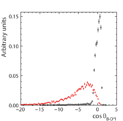
Figure 1: The $\cos\theta_{B\mathchar 45\relax D^{*}\ell}$ distributions for $\bar{B}^{0}\rightarrow D^{*+}\tau^{-}\bar{\nu}_{\tau}$ (solid red circles) and $\bar{B}^{0}\rightarrow D^{*+}\ell^{-}\bar{\nu}_{\ell}$ (open black circles) taken from MC simulation.

IV SIGNAL, NORMALIZATION AND BACKGROUND SEPARATION

To separate reconstructed signal and normalization events, we employ a neural network using the NeuroBayes software package NEUROBAYES . The variables used as inputs to the network are $\cos\theta^{\rm sig}_{B\mathchar 45\relax D^{*}\ell}$, the missing mass squared $M_{\rm miss}^{2}=(2E_{\rm beam}-\sum_{i}E_{i})^{2}/c^{4}-|\sum_{i}\vec{p}_{i}|^{2}/c^{2}$, and the visible energy $E_{\rm vis}=\sum_{i}E_{i}$, where $(E_{i},\vec{p}_{i})$ is the four-momentum of particle $i$ in the $\Upsilon(4S)$ rest frame. The most powerful observable in separating signal and normalization is $\cos\theta^{\rm sig}_{B\mathchar 45\relax D^{*}\ell}$. The neural network is trained using MC samples of signal and normalization events. We will use the neural network classifier as one of the fitting variables for the measurement of ${\cal R}(D^{*})$ without any selection on the neural network classifier. Typically, for a requirement the neural network classifier to be larger than 0.8, 82% of the signal is kept while rejecting 97% of the normalization events.

The dominant background contributions arise from events with misreconstructed $D^{(*)}$ mesons (denoted fakes). The sub-dominant contributions arise from two sources in which $D^{*}$ mesons from both $B_{\rm sig}$ and $B_{\rm tag}$ are correctly reconstructed. One source is $B\rightarrow D^{**}\ell\nu_{\ell}$, where the $D^{**}$ meson decays to $D^{(*)}$ and other particles. The other source is $B\rightarrow X_{c}D^{*}$ events, where one $D^{*}$ meson is correctly reconstructed and the other charmed meson $X_{c}$ decays semileptonically. If the hadrons in the semileptonic $X_{c}$ decay are not identified, such events can mimic signal. Similarly, events in which $X_{c}$ is a $D_{s}^{+}$ meson decaying into $\tau^{+}\nu_{\tau}$ can also mimic signal.

To separate signal and normalization events from background processes, we place a criterion on the sum of the energies of neutral clusters detected in the ECL that are not associated with reconstructed particles, denoted as $E_{\rm ECL}$. To mitigate the effects of photons related to beam background in the energy sum, we only include clusters with energies greater than 50, 100, and 150 MeV, respectively, from the barrel, forward, and backward calorimeter regions, defined in Ref. BELLE . Signal and normalization events peak near zero in $E_{\rm ECL}$, while background events can populate a wider range as shown in Figure 2. We require $E_{\rm ECL}$ to be less than 1.2 GeV.

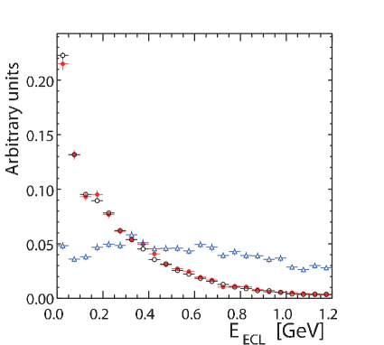
Figure 2: The $E_{\rm ECL}$ distributions for the signal (solid red circles), the normalization (open black circles), and the background (open blue triangles) taken from MC simulation, where the $E_{\rm ECL}$ is defined as the sum of the energies of neutral clusters detected in the ECL that are not associated with reconstructed particles.

V MC CALIBRATION

To improve the accuracy of the MC simulation, we apply a series of calibration factors determined from control sample measurements. The lepton identification efficiencies are separately corrected for electrons and for muons to account for differences between the detector responses in data and MC. Correction factors for lepton identification efficiencies are evaluated as a functions of the momentum and direction of the lepton using $e^{+}e^{-}\rightarrow e^{+}e^{-}\ell^{+}\ell^{-}$ and $J/\psi\rightarrow\ell^{+}\ell^{-}$ decays. We reweight events to account for differing $D^{(*)}$ yields between data and MC.

The differing yields of correctly reconstructed $D^{(*)}$ mesons in data and MC affect the ${\cal R}(D^{*})$ measurement, as it biases the determination of the background contribution. Calibration factors for events with both correctly- and falsely-reconstructed $D$ mesons are estimated for each $D$ meson decay mode using a two-dimensional fit to $M_{D}$. For this calibration, we use samples with all selection criteria other than $D$ mass and $\Delta M$ applied. A two-dimensional PDF is constructed by taking the product of the one-dimensional functions for $M_{D}$. The PDF in each dimension is the sum of a signal component and a background component modelled with a first-order polynomial. The signal component is a triple Gaussian for $D^{0}$ decay modes without a $\pi^{0}$ and a Crystal Ball function CB_FUNCTION plus a Gaussian for $D^{0}$ decay modes with a $\pi^{0}$ and $D^{+}$ decay modes. In this calibration, we do not distinguish signal and tag sides. To estimate calibration factors for specific $D$ decay modes, we fit samples in which one $D$ meson is reconstructed in a specific mode while the other is reconstructed in any signal mode. From the ratios of data to MC samples in signal and background yields, we derive calibration factors of the specific decay mode for events with correctly and falsely reconstructed $D$ mesons. We cannot independently determine calibration factors for all $D$ meson decay modes as we use other decay modes when we calibrate each specific decay mode of a given $D$ meson. To estimate all the calibration factors correctly, we first perform the two-dimensional fit for each decay mode without weighting factors, and then iterate the fits using resultant weighting factors until all calibration factors converge.

Similarly, we estimate calibration factors for events with correctly and falsely reconstructed $D^{*}$ mesons from a two-dimensional fit to $\Delta M$. Calibration factors for events with correctly and falsely reconstructed $D^{*}$ mesons are separately estimated for subsequent decay to $D^{0}$ and $D^{+}$ mesons. For this calibration, we use samples in which one $D^{*}$ meson is reconstructed from $D^{0}\pi^{+}$ and the other $D^{*}$ meson is reconstructed from $D^{+}\pi^{0}$. We apply derived calibration factors to samples, in which both $D^{*}$ mesons are reconstructed from $D^{0}\pi^{+}$, and find good agreement. Eventually, the deviations of the yields between the MC sample and the data reduce from 1.1$\sigma$ to 0.2$\sigma$ for the yields of correctly reconstructed $D^{*}$ mesons and from 8.7$\sigma$ to 0.3$\sigma$ for the yields of falsely reconstructed $D^{*}$ mesons, where $\sigma$ is quadratic sum of statistical error from two-dimensional fit to $\Delta M$ in data and MC.

VI MAXIMUM LIKELIHOOD FIT

We extract the yields of the signal and normalization processes from a two-dimensional extended maximum-likelihood fit to neural network classifier output ${\cal O}_{\mathit{NB}}$ and $E_{\rm ECL}$. The likelihood function consists of five components: signal, normalization, fake $D^{(*)}$ events, $B\rightarrow D^{**}\ell\nu_{\ell}$, and other backgrounds (predominantly from $B\rightarrow X_{c}D^{*}$). The PDFs of all components are determined from MC simulation. There are significant correlations between ${\cal O}_{\mathit{NB}}$ and $E_{\rm ECL}$ in the normalization and background components, but not for the signal. We therefore construct the normalization and background PDFs using two-dimensional histograms and apply a smoothing procedure to account for its limited statistical power SMOOTHING . The signal PDF is the product of one-dimensional histograms in ${\cal O}_{\mathit{NB}}$ and $E_{\rm ECL}$.

Three parameters are floated in the final fit: the yields of the signal, normalization, and $B\rightarrow D^{**}\ell\nu_{\ell}$ components. The yield of fake $D^{(*)}$ events is fixed to the value estimated from sidebands in the $\Delta M$ distribution. Since the PDF shape of fake $D^{(*)}$ events depends on the composition of signal, normalization, $B\rightarrow D^{**}\ell\nu_{\ell}$, and other backgrounds, the relative contributions of these processes to the fake $D^{(*)}$ component are described as a function of the three fit parameters. The yields of other backgrounds are fixed to the values expected from MC simulation. The ratio ${\cal R}(D^{*})$ is given by the formula:

$${\cal R}(D^{*}) = \frac{1}{2{\cal B}(\tau^{-}\rightarrow\ell^{-}\bar{\nu}_{\ell}\nu_{\tau})}\cdot\frac{\varepsilon_{\rm norm}}{\varepsilon_{\rm sig}}\cdot\frac{N_{\rm sig}}{N_{\rm norm}},$$ (3)

where $\varepsilon_{\rm sig(norm)}$ and $N_{\rm sig(norm)}$ are the reconstruction efficiency and yields of signal (normalization) events. We use ${\cal B}(\tau^{-}\rightarrow\ell^{-}\bar{\nu}_{\ell}\nu_{\tau})=0.176\pm 0.003$ as the average of the world averages for $\ell=e$ and $\ell=\mu$ PDG . The ratio of efficiencies, $\varepsilon_{\rm norm}/\varepsilon_{\rm sig}$, is estimated to be $1.289\pm 0.015$ from MC simulation. The difference between reconstruction efficiencies of signal and normalization events arises from their distinct lepton momentum distributions, and the different event criteria on the $D^{*}$ momenta.

To validate the fit procedure, we perform the fitting to multiple subsets of the available MC samples. Furthermore, we validate the fit procedure by a large number of pseudo experiments. We have not observed any bias.

VII PDF VALIDATION

We validate the PDFs used in the fitting procedure by analysing various control samples. For fake $D^{(*)}$ events, we study the $\Delta M$ sidebands, where we find good agreement in both ${\cal O}_{\mathit{NB}}$ and $E_{\rm ECL}$. For $B\rightarrow D^{*}\ell\nu_{\ell}$ decays, we require one $B$ meson to be reconstructed with the hadronic tagging method HADTAG_NEURO and the other $B$ meson reconstructed with the nominal criteria of this analysis. We find good agreement between data and MC in the $E_{\rm ECL}$, $M_{\rm miss}^{2}$, and $E_{\rm vis}$ distributions, but small discrepancies in the $\cos\theta_{B\mathchar 45\relax D^{*}\ell}$ distributions SUPP , which we incorporate as a systematic uncertainty.

VIII SYSTEMATIC UNCERTAINTIES

To estimate the systematic uncertainties on ${\cal R}(D^{*})$, we vary every fixed parameter in turn by one standard deviation and repeat the fit. The systematic uncertainties are summarized in Table 1. The dominant systematic uncertainty arises from the limited size of the MC samples: to estimate this uncertainty, we recalculate PDFs for signal, normalization, fake $D^{(*)}$ events, $B\rightarrow D^{**}\ell\nu_{\ell}$, and other backgrounds by generating toy MC samples from the nominal PDFs according to Poisson statistics and repeat the fit with the new PDFs.

Small discrepancies between the data and MC are found in the $\cos\theta_{B\mathchar 45\relax D^{*}\ell}$ distributions in the hadronic tagged samples. We estimate it as “PDF shape of the normalization in $\cos\theta_{B\mathchar 45\relax D^{*}\ell}$” in Table 1 by correcting the $\cos\theta_{B\mathchar 45\relax D^{*}\ell}$ distribution in MC samples according to the observed discrepancies, and repeating the fit.

The branching fractions of the $B\rightarrow D^{**}\ell\nu_{\ell}$ decay modes and the decays of the $D^{**}$ mesons are not well known and therefore contribute significantly to the total PDF uncertainty for $B\rightarrow D^{**}\ell\nu_{\ell}$ decays. The branching fraction of each $B\rightarrow D^{**}\ell\nu_{\ell}$ decay is varied within its uncertainty. The uncertainties are assumed to be $\pm 6\%$ for $D_{1}$, $\pm 10\%$ for $D_{2}^{*}$, $\pm 83\%$ for $D_{1}^{\prime}$, and $\pm 100\%$ for $D_{0}^{*}$, including the limited knowledge of the $D^{**}$ decays. We also consider the impact of contributions from radially excited $D(2S)$ and $D^{*}(2S)$, where we assume the branching fractions of $B\rightarrow D^{(*)}(2S)\ell\nu_{\ell}$ to be as large as $0.5\%$.

The yield of fake $D^{*}$ events is fixed to the value estimated from sidebands in the $\Delta M$ distribution. We vary this yield within its uncertainties. We also vary the calibration factors for $D$ meson decay modes within their uncertainties for events with falsely reconstructed $D^{(*)}$ events.

The yields of other background processes, predominantly from $B\rightarrow X_{c}D^{*}$ events, are fixed to the values estimated from MC simulation. We consider variations on the yield and shape of the PDF of these background processes within their measured uncertainties. The uncertainties for the $B\rightarrow X_{c}D^{*}$ channels are assumed to be $\pm 8\%$ for $B\rightarrow D_{s}^{*}D^{*-}$, $\pm 14\%$ for $B\rightarrow D_{s}D^{*-}$, $\pm 8\%$ for $B\rightarrow D^{*+}D^{*-}$, and $\pm 10\%$ for $B\rightarrow D^{+}D^{*-}$. Furthermore, we add an uncertainty of $\pm 4\%$ due to the size of the MC sample. We determine the uncertainty from the branching fraction of $D_{s}\rightarrow\tau\nu_{\tau}$ decay (which may peak near the signal in the $E_{\rm ECL}$ distribution) to be negligible.

The reconstruction efficiency ratio of signal to normalization events is varied within its uncertainty, which is limited by the size of the MC samples for signal events.

We include other minor systematic uncertainties from two sources: one related to the parameters that are used for the reweighting of the semileptonic $B\rightarrow D^{(*(*))}\ell\nu_{\ell}$ decays from the ISGW model to the LLSW model; and the other from the branching fraction of $\tau^{-}\rightarrow\ell^{-}\bar{\nu}_{\ell}\nu_{\tau}$ decay PDG . The total systematic uncertainty is estimated by summing the above uncertainties in quadrature.

Table 1: Summary of the systematic uncertainties on ${\cal R}(D^{*})$ for electron and muon modes combined and separated. The uncertainties are relative and are given in percent.

	${\cal R}(D^{*})$ [%]
Sources	$\ell^{\rm sig}=e,\mu$	$\ell^{\rm sig}=e$	$\ell^{\rm sig}=\mu$
MC size for each PDF shape	2.2	2.5	3.9
PDF shape of the normalization in $\cos\theta_{B\mathchar 45\relax D^{*}\ell}$	${}^{+1.1}_{-0.0}$	${}^{+2.1}_{-0.0}$	${}^{+2.8}_{-0.0}$
PDF shape of $B\rightarrow D^{**}\ell\nu_{\ell}$	${}^{+1.0}_{-1.7}$	${}^{+0.7}_{-1.3}$	${}^{+2.2}_{-3.3}$
PDF shape and yields of fake $D^{(*)}$	1.4	1.6	1.6
PDF shape and yields of $B\rightarrow X_{c}D^{*}$	1.1	1.2	1.1
Reconstruction efficiency ratio $\varepsilon_{\rm norm}/\varepsilon_{\rm sig}$	1.2	1.5	1.9
Modeling of semileptonic decay	0.2	0.2	0.3
${\cal B}(\tau^{-}\rightarrow\ell^{-}\bar{\nu}_{\ell}\nu_{\tau})$	0.2	0.2	0.2
Total systematic uncertainty	${}^{+3.4}_{-3.5}$	${}^{+4.1}_{-3.7}$	${}^{+5.9}_{-5.8}$

IX RESULTS

The ${\cal O}_{\mathit{NB}}$ and $E_{\rm ECL}$ projections of the fitted distributions are shown in Figure 3. The yields of signal and normalization events are measured to be $231\pm 23({\rm stat})$ and $2800\pm 57({\rm stat})$, respectively. The ratio ${\cal R}(D^{*})$ is found to be

$${\cal R}(D^{*}) = 0.302\pm 0.030\pm 0.011,$$ (4)

where the first uncertainty is statistical and the second systematic (and likewise for all following results).

We calculate the statistical significance of the signal as $\sqrt{-2\ln({\cal L}_{0}/{\cal L}_{\rm max})}$, where ${\cal L}_{\rm max}$ and ${\cal L}_{0}$ are the maximum likelihood and the likelihood obtained assuming zero signal yield, respectively. We obtain a statistical significance of $13.8\sigma$. We also estimate the compatibility of the measured value of ${\cal R}(D^{*})$ and the SM prediction. The effect of systematic uncertainties is included by convolving the likelihood function with a Gaussian distribution. We conclude that our result is larger than the SM prediction by $1.6\sigma$.

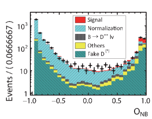
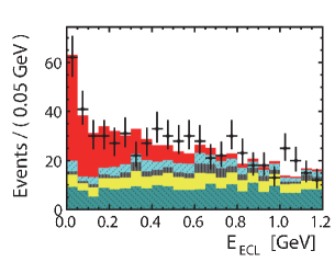
Figure 3: Projections of the fit results with data points overlaid for (left) the neural network classifier output, ${\cal O}_{\mathit{NB}}$, and the $E_{\rm ECL}$ distribution in (center) the signal-enhanced region, ${\cal O}_{\mathit{NB}}>0.8$, and (right) the normalization-enhanced region, ${\cal O}_{\mathit{NB}}<0.8$. The background categories are described in detail in the text, where “others” refers to predominantly $B\rightarrow X_{c}D^{*}$ decays.

X CROSS-CHECKS

To determine the consistency of the measured value of ${\cal R}(D^{*})$ among $\tau$ final states, we divide the data samples by lepton flavor on the signal side and fit them separately. All PDFs for electron and muon channels are separately constructed from the MC samples. The efficiency ratios $\varepsilon_{\rm norm}/\varepsilon_{\rm sig}$ are estimated to be $1.107\pm 0.016$ and $1.591\pm 0.030$ for electron and muon channels of the tau decays, respectively. We obtain

$${\cal R}(D^{*}) = 0.311\pm 0.038\pm 0.013\hskip 5.0pt(\ell^{\rm sig}=e),$$ (5)

$${\cal R}(D^{*}) = 0.304\pm 0.051\pm 0.018\hskip 5.0pt(\ell^{\rm sig}=\mu).$$ (6)

The systematic uncertainties are summarized in Table 1. These two results are consistent with each other.

To study $B\rightarrow D^{**}\ell\nu_{\ell}$ background contributions, we require an additional $\pi^{0}$ with respect to the nominal event selection. In this control sample, we calculate $E^{\prime}_{\rm ECL}$, which is defined as the remaining energy after the energy deposit from the additional $\pi^{0}$ is removed from $E_{\rm ECL}$. The $B\rightarrow D^{**}\ell\nu_{\ell}$ background contributions are extracted from the control samples using the nominal fitting method, replacing $E_{\rm ECL}$ with $E^{\prime}_{\rm ECL}$, which is defined as $E_{\rm ECL}$ without the energy deposit from the additional $\pi^{0}$ SUPP . We find consistent results for the branching fractions of $B\rightarrow D^{**}\ell\nu_{\ell}$ in the control and signal samples.

XI NEW PHYSICS COMPATIBILITY TESTS

Assuming all neutrinos are left-handed, the effective Hamiltonian that contains all possible four-fermion operators for the $b\rightarrow c\tau\nu_{\tau}$ decay can be described as follows SIG_DECAY_MODEL :

$${\cal H}_{\rm eff} = \frac{4G_{F}}{\sqrt{2}}V_{cb}\left[{\cal O}_{V_{1}}+\sum_{X=S_{1},S_{2},V_{1},V_{2},T}C_{X}{\cal O}_{X}\right],$$ (7)

where the four-Fermi operators, ${\cal O}_{X}$, are defined as

$${\cal O}_{S_{1}} = (\bar{c}_{L}b_{R})(\bar{\tau}_{R}\nu_{\tau L}),$$ (8)

$${\cal O}_{S_{2}} = (\bar{c}_{R}b_{L})(\bar{\tau}_{R}\nu_{\tau L}),$$ (9)

$${\cal O}_{V_{1}} = (\bar{c}_{L}\gamma^{\mu}b_{L})(\bar{\tau}_{L}\gamma_{\mu}\nu_{\tau L}),$$ (10)

$${\cal O}_{V_{2}} = (\bar{c}_{R}\gamma^{\mu}b_{R})(\bar{\tau}_{L}\gamma_{\mu}\nu_{\tau L}),$$ (11)

$${\cal O}_{T} = (\bar{c}_{R}\sigma^{\mu\nu}b_{L})(\bar{\tau}_{R}\sigma_{\mu\nu}\nu_{\tau L}),$$ (12)

and the $C_{X}$ parameters are the Wilson coefficients of ${\cal O}_{X}$. We investigate the compatibility of the data samples with new physics using a model-independent approach, separately examining the impact of each operator. In each new-physics scenario, we take into account changes in the efficiency and fit PDF shapes using dedicated signal simulation. We set the Wilson coefficients to be real in all cases. Since ${\cal O}_{V_{1}}$ is just the SM operator, it would change only ${\cal R}(D^{*})$, but not the kinematic distributions. In the type-II two-Higgs doublet model (2HDM), the relevant Wilson coefficients are given as $C_{S_{1}}=-m_{b}m_{\tau}\tan^{2}\beta/m_{H^{+}}^{2}$ and $C_{S_{2}}=-m_{c}m_{\tau}/m_{H^{+}}^{2}$, where $\tan\beta$ is the ratio of the vacuum expectation values of the two Higgs doublets, and $m_{b}$, $m_{c}$, $m_{\tau}$, and $m_{H^{+}}$ are the masses of the $b$ quark, $c$ quark, $\tau$ lepton, and charged Higgs boson. Since the contribution from $C_{S_{2}}$ is almost negligibly small except for the light charged Higgs boson, we neglect the contribution from $C_{S_{2}}$ in the type-II 2HDM.

Various leptoquark models have been presented to explain anomalies in ${\cal R}(D^{(*)})$ in Ref. LQ1 . In addition to the model-independent study, we study two representative models: $R_{2}$ and $S_{1}$. Model $R_{2}$ contains scalar leptoquarks of the type $(3,2)_{7/6}$ using the notation $(SU(3)_{c},SU(2)_{L})_{Y}$, where $SU(3)_{c}$ is the representation under the generators of QCD, $SU(2)_{L}$ is the representation under the generators of weak isospin, and $Y$ is the weak hypercharge. Model $S_{1}$ contains leptoquarks of the type $(3^{*},1)_{1/3}$. In these leptoquark models, the relevant Wilson coefficients are related by $C_{S_{2}}=+7.8C_{T}$ for the $R_{2}$-type leptoquark model and $C_{S_{2}}=-7.8C_{T}$ for the $S_{1}$-type leptoquark model at the $b$ quark mass scale, assuming a leptoquark mass scale of 1 TeV/$c^{2}$. Although the $V_{1}$ operator can appear independently of the $S_{2}$ and $T$ operators in the $S_{1}$-type leptoquark model, we assume no contribution from the $V_{1}$ operator in this study.

Figure 4 shows the dependence of the efficiency and measured value of ${\cal R}(D^{*})$ as a function of the values of the respective parameters in the type-II 2HDM and the $R_{2}$-type leptoquark model. Efficiency variations for other scenarios are shown in Ref. SUPP . We find that efficiencies increase by up to 17% for ${\cal O}_{V_{2}}$ and ${\cal O}_{T}$, mainly due to the variation of the $D^{*}$ momentum distribution. Similarly, the efficiencies increase by up to 16% and 11% in $R_{2}$- and $S_{1}$-type leptoquark models, respectively, which include contributions from ${\cal O}_{T}$. In other scenarios, the efficiency variation is 6% or less. Figure 5 shows the dependency of the measured values of ${\cal R}(D^{*})$ on the values of the respective parameters in the type-II 2HDM and the $R_{2}$-type leptoquark model. The allowed regions with 68% confidence level (C.L.) of the respective parameters are summarized in Table 2.

Table 2: Allowed regions with 68% C.L. of Wilson coefficients SIG_DECAY_MODEL . $-4.25<C_{S_{1}}<-3.09$ corresponds to $0.65$ GeV${}^{-1}<\tan\beta/m_{H^{+}}<0.76$ GeV^-1 in type-II 2HDM, where $m_{b}=4.20$ GeV/$c^{2}$, $m_{c}=0.901$ GeV/$c^{2}$ QUARK_MASS and $m_{\tau}=1.77682$ GeV/$c^{2}$ PDG are used.

Models or operators	Parameters	Allowed regions
		(68% C.L.)
${\cal O}_{S_{1}}$	$C_{S_{1}}$	$[-4.25,-3.09],[+0.44,+1.57]$
${\cal O}_{S_{2}}$	$C_{S_{2}}$	$[-1.56,-0.43],[+3.12,+4.28]$
${\cal O}_{V_{1}}$	$C_{V_{1}}$	$[-2.15,-2.03],[+0.05,+0.15]$
${\cal O}_{V_{2}}$	$C_{V_{2}}$	$[-0.17,0.00],[+1.83,+1.96]$
${\cal O}_{T}$	$C_{T}$	$[-0.06,-0.01],[+0.34,+0.39]$
$R_{2}$-type leptoquark	$C_{T}(=+C_{S_{2}}/7.8)$	$[-0.05,-0.01],[+0.34,+0.38]$
$S_{1}$-type leptoquark	$C_{T}(=-C_{S_{2}}/7.8)$	$[-0.07,-0.01],[+0.22,+0.28]$

In Refs. BABAR_HAD_NEW and BELLE_HAD_NEW , the $q^{2}\equiv(p_{B}-p_{D^{*}})^{2}$ spectra are examined in order to study the effects of new physics beyond the SM. Since $q^{2}$ cannot be calculated here due to the neutrino in the decay of the $B_{\rm tag}$, we use instead the momenta of the $D^{*}$ and the $\ell$ in $B_{\rm sig}$ at the $\Upsilon(4S)$ rest frame. Figure 6 shows the momentum distributions of the background-subtracted data in the region of ${\cal O}_{\mathit{NB}}>0.8$ and $E_{\rm ECL}<0.5$ GeV for the SM, type-II 2HDM with $\tan\beta/m_{H^{+}}=0.7$ GeV^-1, and the $R_{2}$-type leptoquark model with $C_{T}=+0.36$. The PDF shapes of background events are taken from MC simulation and normalized to the yields obtained by the fitting. Table 3 shows $p$ values for all scenarios, where we include only the statistical uncertainty. We find our data are compatible with the SM and additional contributions from scalar and vector operators; large additional contributions from tensor operator or the $R_{2}$- and $S_{1}$-type leptoquark models are disfavored.

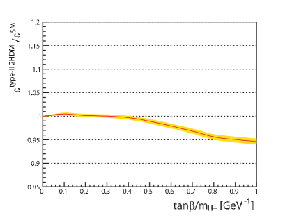
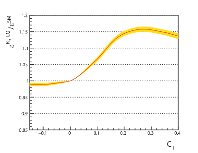
Figure 4: The efficiencies for (left) the type-II 2HDM and (right) $R_{2}$-type leptoquark model with respect to the SM value.

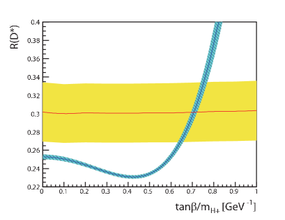
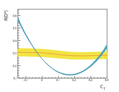
Figure 5: The measured values of ${\cal R}(D^{*})$ for (left) the type-II 2HDM and (right) $R_{2}$-type leptoquark models, where central values are given as the solid (red) curves and the $1\sigma$ uncertainties are given as the shaded (yellow) regions. The theoretical predictions and their $1\sigma$ uncertainties are shown as solid (blue) curves and hatched (light blue) regions, respectively SIG_DECAY_MODEL .

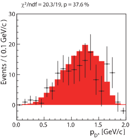
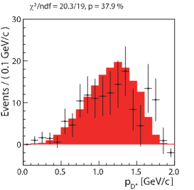
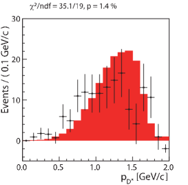
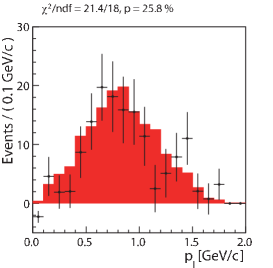
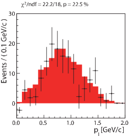
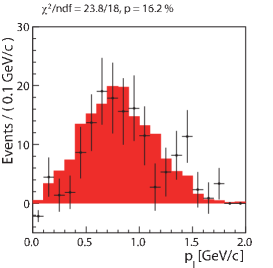
Figure 6: Background-subtracted momentum distributions of $D^{*}$ (top) and $\ell$ (bottom) in the region of ${\cal O}_{\mathit{NB}}>0.8$ and $E_{\rm ECL}<0.5$ GeV for (left) the SM, (center) the type-II 2HDM with $\tan\beta/m_{H^{+}}=0.7$ GeV^-1, and (right) $R_{2}$-type leptoquark model with $C_{T}=+0.36$. The points and the shaded histograms correspond to the measured and expected distributions, respectively. The expected distributions are normalized to the number of detected events.

Table 3: $p$ values for each scenario from the momentum distributions of the $D^{*}$ or the lepton on the signal side in the $\Upsilon(4S)$ rest frame, where we include only the statistical uncertainty.

		$p$ values [%]
Model or operator	Parameter	$p_{D^{*}}$	$p_{\ell}$
SM		37.6	25.8
Type-II 2HDM	$\frac{\tan\beta}{m_{H^{+}}}=0.7$ GeV-1	37.9	22.5
${\cal O}_{V_{2}}$	$C_{V_{2}}=+1.88$	24.1	18.6
${\cal O}_{T}$	$C_{T}=+0.36$	0.9	19.2
$R_{2}$-type leptoquark model	$C_{T}=+0.36$	1.4	16.2
$S_{1}$-type leptoquark model	$C_{T}=+0.26$	1.1	15.4

XII CONCLUSION

In conclusion, we report the first measurement of ${\cal R}(D^{*})$ with a semileptonic tagging method using a data sample containing $772\times 10^{6}B\bar{B}$ pairs collected with the Belle detector. The result is

$${\cal R}(D^{*}) = 0.302\pm 0.030\pm 0.011,$$ (13)

which is within $1.6\sigma$ of the SM prediction including systematic uncertainties, and is in good agreement with other measurements by Belle BELLE_INCLUSIVE_OBSERVATION ; BELLE_INCLUSIVE ; BELLE_HAD_NEW , B A B AR BABAR_HAD_NEW , and LHCb LHCB_RESULT . The result is statistically independent of earlier Belle measurements. We investigate the compatibility of the data samples with new physics in a model-independent method by adding the operators one by one. We also study two types of leptoquark models. We find our data allow the additional contributions from scalar and vector operators while disfavoring large additional contributions from a tensor operator with $+0.34<C_{T}<+0.39$, an $R_{2}$-type leptoquark model with $+0.34<C_{T}<+0.38$, or an $S_{1}$-type leptoquark model with $+0.22<C_{T}<+0.28$, when considering the impact on the decay kinematics.

XIII ACKNOWLEDGEMENTS

We thank Y. Sakaki, R. Watanabe, and M. Tanaka for their invaluable suggestions. This work was supported in part by a Grant-in-Aid for JSPS Fellows (No.13J03438) and a Grant-in-Aid for Scientific Research (S) “Probing New Physics with Tau-Lepton” (No.26220706). We thank the KEKB group for the excellent operation of the accelerator; the KEK cryogenics group for the efficient operation of the solenoid; and the KEK computer group, the National Institute of Informatics, and the PNNL/EMSL computing group for valuable computing and SINET4 network support. We acknowledge support from the Ministry of Education, Culture, Sports, Science, and Technology (MEXT) of Japan, the Japan Society for the Promotion of Science (JSPS), and the Tau-Lepton Physics Research Center of Nagoya University; the Australian Research Council; Austrian Science Fund under Grant No. P 22742-N16 and P 26794-N20; the National Natural Science Foundation of China under Contracts No. 10575109, No. 10775142, No. 10875115, No. 11175187, No. 11475187 and No. 11575017; the Chinese Academy of Science Center for Excellence in Particle Physics; the Ministry of Education, Youth and Sports of the Czech Republic under Contract No. LG14034; the Carl Zeiss Foundation, the Deutsche Forschungsgemeinschaft, the Excellence Cluster Universe, and the VolkswagenStiftung; the Department of Science and Technology of India; the Istituto Nazionale di Fisica Nucleare of Italy; the WCU program of the Ministry of Education, National Research Foundation (NRF) of Korea Grants No. 2011-0029457, No. 2012-0008143, No. 2012R1A1A2008330, No. 2013R1A1A3007772, No. 2014R1A2A2A01005286, No. 2014R1A2A2A01002734, No. 2015R1A2A2A01003280, No. 2015H1A2A1033649; the Basic Research Lab program under NRF Grant No. KRF-2011-0020333, Center for Korean J-PARC Users, No. NRF-2013K1A3A7A06056592; the Brain Korea 21-Plus program and Radiation Science Research Institute; the Polish Ministry of Science and Higher Education and the National Science Center; the Ministry of Education and Science of the Russian Federation and the Russian Foundation for Basic Research; the Slovenian Research Agency; Ikerbasque, Basque Foundation for Science and the Euskal Herriko Unibertsitatea (UPV/EHU) under program UFI 11/55 (Spain); the Swiss National Science Foundation; the Ministry of Education and the Ministry of Science and Technology of Taiwan; and the U.S. Department of Energy and the National Science Foundation. This work is supported by a Grant-in-Aid from MEXT for Science Research in a Priority Area (“New Development of Flavor Physics”) and from JSPS for Creative Scientific Research (“Evolution of Tau-lepton Physics”).

XIV SUPPLEMENTAL MATERIAL

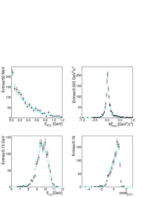
Figure 7: Distributions of $E_{\rm ECL}$ (top left), $M_{\rm miss}^{2}$ (top right), $E_{\rm vis}$ (bottom left), and $\cos\theta_{B\mathchar 45\relax D^{*}\ell}$ (bottom right) in the hadronic tagged sample. The signal side is reconstructed from the decay $\bar{B}^{0}\rightarrow D^{*+}\ell^{-}\bar{\nu}_{\ell}$ followed by $D^{*+}\rightarrow D^{0}\pi^{+}$. The black dots with error bars show the data and the light blue rectangles show the normalized MC samples.

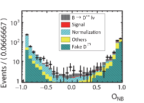
(a) ${\cal O}_{\mathit{NB}}$ distribution.

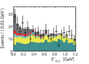
(b) $E^{\prime}_{\rm ECL}$ distribution with $B\rightarrow D^{**}\ell\nu_{\ell}$-enhanced ${\cal O}_{\mathit{NB}}$ region (${\cal O}_{\mathit{NB}}>0.0$).

(c) $E^{\prime}_{\rm ECL}$ distribution with normalization-enhanced ${\cal O}_{\mathit{NB}}$ region (${\cal O}_{\mathit{NB}}<0.0$).

Figure 8: Projection of the fit results of control samples with data points overlaid. In the control samples, we require $\pi^{0}$ in addition to the nominal event selection. $E^{\prime}_{\rm ECL}$ is defined as $E_{\rm ECL}$ excluded from energy deposit from additional $\pi^{0}$.

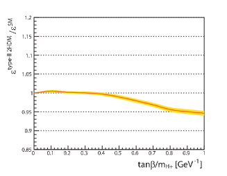
(a) Type-II 2HDM.

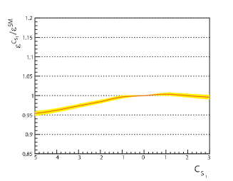
(b) SM with adding contribution from ${\cal O}_{S_{1}}$.

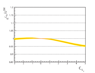
(c) SM with adding contribution from ${\cal O}_{S_{2}}$.

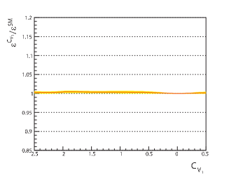
(d) SM with adding contribution from ${\cal O}_{V_{1}}$.

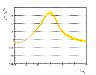
(e) SM with adding contribution from ${\cal O}_{V_{2}}$.

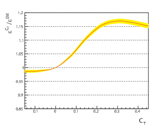
(f) SM with adding contribution from ${\cal O}_{T}$.

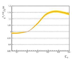
(g) $R_{2}$-type leptoquark model.

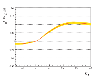
(h) $S_{1}$-type leptoquark model.

Figure 9: Efficiency with respect to the SM value.

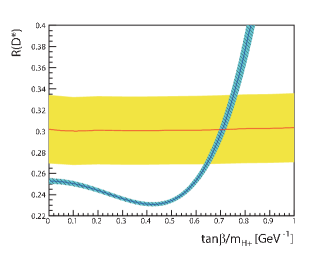
(a) Type-II 2HDM.

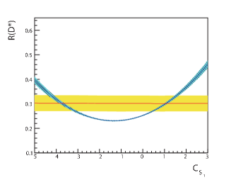
(b) SM with adding contribution from ${\cal O}_{S_{1}}$.

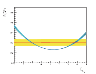
(c) SM with adding contribution from ${\cal O}_{S_{2}}$.

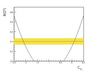
(d) SM with adding contribution from ${\cal O}_{V_{1}}$.

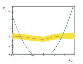
(e) SM with adding contribution from ${\cal O}_{V_{2}}$.

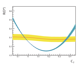
(f) SM with adding contribution from ${\cal O}_{T}$.

(g) $R_{2}$-type leptoquark model.

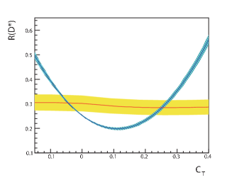
(h) $S_{1}$-type leptoquark model.

Figure 10: Measured values of ${\cal R}(D^{*})$ and their ($1\sigma$) uncertainties are shown by solid (red) curve and shaded (yellow) region. Theoretical predictions and their ($1\sigma$) uncertainties are shown by solid (blue) curve and hatched (light blue) region.

(a) SM.

(b) Type-II 2HDM with $\tan\beta/m_{H^{+}}=0.7$ GeV^-1.

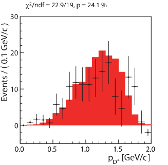
(c) SM with adding contribution from ${\cal O}_{V_{2}}$ ($C_{V_{2}}=+1.88$).

(d) SM with adding contribution from ${\cal O}_{T}$ ($C_{T}=+0.36$).

(e) $R_{2}$-type leptoquark model with $C_{T}=+0.36$.

(f) $S_{1}$-type leptoquark model with $C_{T}=+0.26$.

Figure 11: Background-subtracted $D^{*}$ momentum distributions in the region of ${\cal O}_{\mathit{NB}}>0.8$ and $E_{\rm ECL}<0.5$ GeV. The points and the shaded histograms correspond to the measured and expected distributions, respectively. The expected distributions are normalized to the number of detected events.

(a) SM.

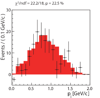
(b) Type-II 2HDM with $\tan\beta/m_{H^{+}}=0.7$ GeV^-1.

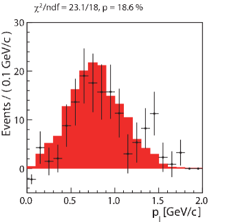
(c) SM with adding contribution from ${\cal O}_{V_{2}}$ ($C_{V_{2}}=+1.88$).

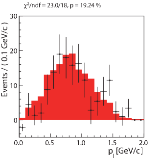
(d) SM with adding contribution from ${\cal O}_{T}$ ($C_{T}=+0.36$).

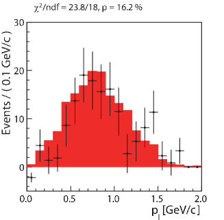
(e) $R_{2}$-type leptoquark model with $C_{T}=+0.36$.

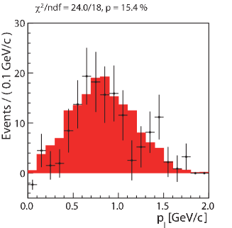
(f) $S_{1}$-type leptoquark model with $C_{T}=+0.26$.

Figure 12: Background-subtracted lepton momentum distributions in the region of ${\cal O}_{\mathit{NB}}>0.8$ and $E_{\rm ECL}<0.5$ GeV. The points and the shaded histograms correspond to the measured and expected distributions, respectively. The expected distributions are normalized to the number of detected events.

References

(1)
Charge-conjugate decays are implied throughout this paper,
unless otherwise stated.
(2)
H. Itoh, S. Komine, and Y. Okada,
Prog. Theor. Phys. 114, 179 (2005).
(3)
M. Tanaka, Z. Phys. C 67, 321 (1995).
(4)
Y. Sakaki, R. Watanabe, M. Tanaka, and A. Tayduganov,
Phys. Rev. D 88, 094012 (2013).
(5)
S. Fajfer, J.F. Kamenik, and I. Nisandzic,
Phys. Rev. D 85, 094025 (2012).
(6)
J.F. Kamenik, and F. Mescia,
Phys. Rev. D 78, 014003 (2008).
(7)
J.P. Lees et al.
(B A B
AR Collaboration),
Phys. Rev. Lett. 109, 101802 (2012);
J.P. Lees et al.
(B A B
AR Collaboration),
Phys. Rev. D 88, 072012 (2013).
(8)
J.A. Bailey et al. (Fermilab Lattice and MILC Collaborations),
Phys. Rev. D 92, 034506 (2015).
(9)
H. Na, C.M. Bouchard, G.P. Lepage, C. Monahan, and J. Shigemitsu,
Phys. Rev. D 92, 054510 (2015).
(10)
A. Matyja et al. (Belle Collaboration),
Phys. Rev. Lett. 99, 191807 (2007).
(11)
A. Bozek et al. (Belle Collaboration),
Phys. Rev. D 82, 072005 (2010).
(12)
M. Huschle et al. (Belle Collaboration),
Phys. Rev. D 92, 072014 (2015).
(13)
R. Aaij et al. (LHCb Collaboration),
Phys. Rev. Lett. 115, 111803 (2015).
(14)
Y. Amhis et al. (Heavy Flavor Averaging Group), arXiv:1412.7515
and online update at
http://www.slac.stanford.edu/xorg/hfag/.
(15)
B. Kronenbitter et al. (Belle Collaboration),
Phys. Rev. D 92, 051102(R) (2015).
(16)
B. Aubert et al.
(B A B
AR Collaboration),
Phys. Rev. D 81, 051101(R) (2010).
(17)
A. Abashian et al. (Belle Collaboration),
Nucl. Instrum. Methods Phys. Res., Sect. A 479, 117 (2002);
also see the detector section in J. Brodzicka et al., Prog. Theor. Exp. Phys. (2012) 04D001.
(18)
S. Kurokawa and E. Kikutani,
Nucl. Instrum. Methods Phys. Res., Sect. A 499, 1 (2003),
and other papers included in this volume;
T. Abe et al., Prog. Theor. Exp. Phys. (2013) 03A001
and following articles up to 03A011.
(20)
R. Brun et al.,
GEANT3.21,
CERN Report No. DD/EE/84-1, (1984) (unpublished).
(21)
M. Tanaka and R. Watanabe,
Phys. Rev. D 87, 034028 (2013).
(22)
D. Scora and N. Isgur,
Phys. Rev. D 52, 2783 (1995).
(23)
A.K. Leibovich, Z. Ligeti, I.W. Stewart, and M.B. Wise,
Phys. Rev. D 57, 308 (1998).
(24)
K. Hanagaki, H. Kakuno, H. Ikeda, T. Iijima, and T. Tsukamoto,
Nucl. Instrum. Methods Phys. Res., Sect. A 485, 490 (2002).
(25)
A. Abashian et al.,
Nucl. Instrum. Methods Phys. Res., Sect. A 491, 69 (2002).
(26)
E. Nakano,
Nucl. Instrum. Methods Phys. Res., Sect. A 494, 402 (2002).
(27)
K.A. Olive et al (Particle Data Group),
Chin. Phys. C 38, 090001 (2014).
(28)
M. Feindt and U. Kerzel,
Nucl. Instrum. Methods Phys. Res., Sect. A 559, 190 (2006).
(29)
T. Skwarnicki, Ph.D. Thesis,
Institute for Nuclear Physics,
Krakow 1986;
DESY Internal Report,
DESY F31-86-02 (1986).
(30)
J.H. Friedman, Data Analysis Techniques for High Energy Particle Physics,
in: Proc. 1974 CERN School of Computing, CERN 74-23 (1974).
(31)
M. Feindt, F. Keller, M. Kreps, T. Kuhr, S. Neubauer, D. Zander, and A. Zunpac,
Nucl. Instrum. Methods Phys. Res., Sect. A 654, 432 (2011).
(32)
See supplemental Material for
comparison of the data and MC distribution in hadronic tagged samples,
fit figures of the controls samples for backgrounds,
efficiency variation, measured value of ,
and background-subtracted momenta distributions of and lepton.
(33)
Z. z. Xing, H. Zhang and S. Zhou,
Phys. Rev. D 77, 113016 (2008).