Cosmological simulations of Milky Way-sized galaxies

Abstract

We introduce a new set of eight Milky Way-sized cosmological simulations performed using the AMR code ART + Hydrodynamics in a $\Lambda$CDM cosmology. The set of zoom-in simulations covers present-day virial masses that range from $8.3\times 10^{11}\mbox{$M_{\odot}$}$ to $1.56\times 10^{12}\mbox{$M_{\odot}$}$ and is carried out with our simple but effective deterministic star formation (SF) and “explosive” stellar feedback prescriptions. The work is focused on showing the goodness of the simulated set of “field” Milky Way-sized galaxies. To this end, we compare some of the predicted physical quantities with the corresponding observed ones. Our results are as follows. (a) In agreement with some previous works, we found circular velocity curves that are flat or slightly peaked. (b) All simulated galaxies with a significant disk component are consistent with the observed Tully-Fisher, radius-mass, and cold gas-stellar mass correlations of late-type galaxies. (c) The disk-dominated galaxies have stellar specific angular momenta in agreement with those of late-type galaxies, with values around $10^{3}$ km/s/kpc. (d) The SF rates at $z=0$ of all runs but one are comparable to those estimated for the star-forming galaxies. (e) The two most spheroid-dominated galaxies formed in halos with late active merger histories and late bursts of SF, but the other run that ends also as dominated by an spheroid, never had major mergers. (f) The simulated galaxies lie in the semi-empirical stellar-to-halo mass correlation of local central galaxies, and those that end up as disk dominated, evolve mostly along the low-mass branch of this correlation. Moreover, the baryonic and stellar mass growth histories of these galaxies are proportional to their halo mass growth histories since the last 6.5–10 Gyr. (g) Within the virial radii of the simulations, $\approx 25-50\%$ of the baryons are missed; the amount of gas in the halo is similar to the one in stars in the galaxy, and most of this gas is in the warm-hot phase. (h) The $z\sim 0$ vertical gas velocity dispersion profiles, $\sigma_{z}$($r$), are nearly flat and can be mostly explained by the kinetic energy injected by stars. The average values of $\sigma_{z}$ increase at higher redshifts, following roughly the shape of the SF history.

1. Introduction

The galaxy formation and evolution, circumscribed to the hierarchical structure formation scenario, is a fascinating problem. It is a complex phenomenon that involves many physical processes and scales, from the formation of the dark and gaseous halos at scales of tens to hundreds of kpc to the formation of stars in giant molecular clouds at scales of dozens of pc (e.g., McKee & Ostriker, 2007), passing through the formation of supermassive black holes at the center of massive galaxies at scales of $10^{-3}$ pc or less (e.g., Volonteri, 2010), with their corresponding stage of active galactic nuclei (AGN). They are accompanied by a variety of large-scale feedback effects such as, for example, supernovae (SNe) explosions and AGN outflows. Yet, we can encounter larger scales and new phenomena related to galaxy formation during the formation of groups and clusters of galaxies (e.g., Kravtsov & Borgani, 2012).

It has been long known that disks, as observed, should form when gas cools, condenses and collapses, within dark matter halos, while conserving its angular momentum, obtained through external torques (White & Rees, 1978; Fall & Efstathiou, 1980; Mo et al., 1998; Firmani & Avila-Reese, 2000). Yet, until recently, forming extended disk galaxies with flat rotation curves in hydrodynamic simulations, in a hierarchical cosmogony, was a challenge (e.g., Mayer et al., 2008).

Earlier works show that disks could be produced in simulations without difficulty but they inevitably ended up with too little (specific) angular momentum and too much stellar mass at the center of the galaxy (Navarro & Benz, 1991; Katz & Gun, 1991; Navarro & White, 1994, 1995; Somer-Larsen et al., 1999). The problem was that, because of an inefficient feedback or poor resolution or both, “clumps” (composed of gas, stars and dark matter) were too much concentrated by the time they were accreted by a halo/galaxy. The result, at the end, was that this lumpy mass lost most of their orbital angular momentum by a physical process called dynamical friction (e.g., Navarro & Benz, 1991). Later works, with better resolution and/or a more effective stellar feedback improved on this by producing more extended disks and less massive spheroids (Abadi et al., 2003; Somer-Larsen et al., 2003; Governato et al., 2004).

The relatively recent success on forming realistic galaxies can be attributed to some degree to resolution but mainly to a better understanding of the processes that play a major role in the classical overcooling (White & Rees, 1978; Dekel & Silk, 1986; White & Frenk, 1991) and angular momentum (e.g., Mayer et al., 2008) problems. Since the pioneer works of, for example, Navarro & Benz (1991) and Navarro & White (1994), it was clear that to avoid transforming most of the gas into stars a kind of stellar feedback was needed. This source of energy (and momentum) not only could avoid the overcooling of the gas but it could also solve the angular momentum problem by puffing the gas in the clumps up, making it less susceptible to the loss of angular momentum. It was soon realized that in order to do its job the feedback needs to be efficient. Most of works in the recent years get this in one way or another (Guedes et al., 2011; Brook et al., 2012; Governato et al., 2012; Agertz et al., 2013; Hopkins et al., 2014). For example, in a number of works the thermal feedback becomes efficient by delaying artificially, for about $\sim 10^{7}$yr, the cooling of the gas that surrounds the newly formed stellar particle (e.g., Thacker & Couchman, 2000; Stinson et al., 2006; Governato et al., 2007; Agertz et al., 2011; Colín et al., 2010; Piontek & Steinmetz, 2011; Guedes et al., 2011; Teyssier et al., 2013). In this recipe, further star formation (SF) is stopped by the high temperatures and low densities attained by the gas, as a result of turning off the cooling.

Another way of making the feedback efficient is by depositing momentum (kinetic energy) directly into the gas which, unlike the thermal energy, can not be radiated away (Navarro & White, 1993; Springel & Hernquist, 2003; Scannapieco et al., 2006; Oppenheimer & Dave, 2008; Marinacci et al., 2014). This wind method is somehow artificial in the sense that the kick is put by hand and because the wind particles are temporary decoupled from the hydrodynamic interaction. Traditionally, stellar feedback has been associated with the injection of energy only by SNe and in some cases with both SNe and stellar wind by massive stars (Somer-Larsen et al., 2003; Kravtsov, 2003), but very recently some kind of “early” feedback has also been incorporated (Stinson et al., 2013; Hopkins et al., 2014; Trujillo-Gomez et al., 2015). This feedback begins few millions of years before the first SN explodes and it includes radiation pressure (Krumholz et al., 2014) and photoheating by the ionizing radiation of massive stars. This latter has been shown can significantly affect the structure of molecular clouds and in some cases destroy them (Walch et al., 2012; Colín et al., 2013; Lopez et al., 2014). On the other hand, results from Trujillo-Gomez et al. (2015) show that radiation pressure alone has a small effect on the total stellar mass content, but see Hopkins et al. (2014). Nowadays these effects and others, such us cosmic rays (Salem et al., 2014) and turbulence in molecular clouds, are slowly being incorporated in the simulations of galaxy formation.

The MW-sized galaxies are special in the sense that they occupy the peak of the stellar mass growth efficiency within dark matter (DM) halos measured through the $\mbox{$M_{s}$}/\mbox{$M_{\rm vir}$}$ fraction (e.g., Avila-Reese & Firmani, 2011). For less massive galaxies, this efficiency decreases because of the global effects of SN-driven outflows, and for more massive ones, because of the long cooling times of the shock heated gas during the virialization of massive halos and the feedback from luminous AGNs (for a recent review on these processes see Somerville & Dave, 2015). Therefore, since the baryonic mass assembly of MW-sized galaxies is less affected by these astrophysical processes, the shape of their mass assembly history is expected not to deviate dramatically from the way their halos are assembled (see e.g., Conroy & Wechsler, 2009; Firmani et al., 2010; Behroozi et al., 2013a; Moster et al., 2013), being then interesting objects to constrain the $\Lambda$CDM cosmology. Moreover, being these galaxies less susceptible to the large-scale effects of stellar and AGN feedback, they are optimal to probe simple models of large-scale SF and self-regulation, where the generation of turbulence (traced by the cold gas velocity dispersion) and its dissipation in the ISM are key ingredients.

The aim of this work is to introduce a new suite of zoom-in Milky Way (MW) sized simulations run with the N-body + Hydrodynamic ART code (Kravtsov, 2003) and with the SF and stellar feedback prescription implemented for the first time in (Colín et al., 2010, see also Avila-Reese et al. 2011a), and used recently in Roca-Fàbrega et al. (2016) for the “Garrotxa” simulations. Here we use the same $n_{\rm SF}$ and $\epsilon_{\rm SF}$ values as in the latter paper. The dark matter (DM) halos were drawn from a 50 $h^{-1}$Mpc on a side box and have each about 1 million DM particles and cells within their virial radii. The spatial resolution, the side of the cell in the maximum level of refinement, is 136 pc. The runs use a deterministic SF approach; that is, stellar particles form every time gas satisfies certain conditions, with a conversion of gas to stars of 65%. Immediately after they are born, they dump $2\times 10^{51}$ ergs of thermal energy, for every star $>8\mbox{$M_{\odot}$}$, to the gas in the cell where the particle is located, rising its temperature to several $10^{7}\ \mbox{K}$. This high temperature value comes from the high SF efficiency we have assumed and from the fact that all the injected energy is concentrated in time and space (see subsection 4.3). We sometimes call this form of stellar feedback “explosive”, as opposed to the typical assumed feedback consisting of a continuous supply of thermal energy for about 40 Myr (e.g., Ceverino & Klypin, 2009). At this high temperature, the cooling time is much longer than the crossing time (Dalla Vecchia & Schaye, 2012) and so, the differences in the galaxies simulated under the assumption of a delayed cooling and those that do not consider it, are not expected to be significant.

From our sample of eight simulated halos/galaxies, we distinguish four that are clearly disk dominated. Two more have kinematic bulge-to-disk (B/D) ratios of 1.3 and 2.3. The other two had a violent late assembly phase and ended up with B/D ratios of 3 and 10. Here, we study the evolution of the specific angular momentum and the stellar-to-halo mass fraction, $\mbox{$M_{s}$}/\mbox{$M_{\rm vir}$}$, as a function of stellar mass. As usual in this kind of studies, we also compute the circular velocity profiles and the SF histories. The MW-sized galaxies simulated here present realistic $\mbox{$M_{s}$}/\mbox{$M_{\rm vir}$}$ fractions and are consistent with several observational correlations. We find, in agreement with our previous studies (e.g., González-Samaniego et al., 2014), nearly flat circular velocity curves. However, contrary to our results on the low-mass galaxies (Avila-Reese et al., 2011; González-Samaniego et al., 2014), and to some degree also on the MW-sized galaxy of Roca-Fàbrega et al. (2016), here our predicted $\mbox{$M_{s}$}/\mbox{$M_{\rm vir}$}$ values agree with those determined by semi-empirical methods.

The suite of MW-sized galaxies introduced here will be used elsewhere to study in detail the spatially-resolved SF and stellar mass growth histories with the aim to compare the results with look-back time studies and fossil record inferences from observational surveys like MaNGA/SDSS-IV (Bundy et al., 2015). They also will be used to study observational biases after post-processing them to include dust and spectral energy distributions to each stellar particle, and by further performing mock observations.

This paper is organized as follows. In Section 2, we describe the code, the SF and feedback prescriptions, as well as the simulations. In Section 3, we put our simulated galaxies into an observational context by presenting their circular velocity curves, and by comparing the predicted galaxy properties and correlations with observations. Then, we estimate the morphology of our simulated galaxies and present the spatial distribution of light in some color bands. Finally, in the rest of the Section 3 we present: (i) the halo mass aggregation and specific angular momentum evolution of the runs, (ii) the $M_{s}$/$M_{\rm vir}$ ratios and their evolution, (iii) the gas-to-stellar mass ratios, and (iv) the cold gas velocity dispersion profiles. In Section 4, we discuss the resolution issue and the validity our “explosive” stellar feedback. We also discuss the implications of the the dark/stellar mass assembly of our simulated galaxies, as well as the role of the SN feedback as the driver of turbulence and self-regulated SF in the disk. Our conclusions are given in in Section 5.

2. Numerical Methodology

2.1. The Code

The numerical simulations used in this work were run using the N-body + hydrodynamic Adaptive Refinement Tree (ART) code (Kravtsov et al., 1997; Kravtsov, 2003). The code incorporates a variety of physical processes that are essential to the modeling of galaxy formation such as gas cooling, SF, stellar feedback, advection of metals, and a UV heating background source. The Compton heating/cooling, atomic and molecular cooling, and UV heating from a cosmological background radiation (Haardt & Madau, 1996), are all included in the computation of the cooling/heating rates. These are tabulated for a temperature range of $10^{2}<T<10^{9}\ \mbox{K}$ and a grid of densities, metallicities, and redshifts using the CLOUDY code (Ferland et al., 1998, version 96b4).

2.2. Star formation and stellar feedback

Since the subgrid physics of SF and stellar feedback implemented in the code is discussed in detail in Colín et al. (2010) (see also Avila-Reese et al., 2011; Colín et al., 2013, 2015; Roca-Fàbrega et al., 2016), here we only give a brief summary. In the code, a cell form a stellar particle (hereafter SP, unless otherwise stated) if they are dense and cool enough; that is, if $T<\mbox{{$T_{\rm SF}$}}$ and $\rho_{g}>\mbox{$\rho_{\rm SF}$}$, where $T$ and $\rho_{g}$ are the temperature and density of the gas, respectively, and $T_{\rm SF}$ and $\rho_{\rm SF}$ are the temperature and density threshold, respectively. Here, we use the same values of $T_{\rm SF}$ and $n_{\rm SF}$ parameters as in Roca-Fàbrega et al. (2016); namely, 9000 K and 1 cm^-3, respectively, where $n_{\rm SF}$ is the density threshold in hydrogen atoms per cubic centimeter. In practice, the temperature requirement is almost always satisfied once the gas density reaches a value above $\rho_{\rm SF}$. In the present scheme of our subgrid SF+feedback recipe the outcome of the simulation is sensitive to $n_{\rm SF}$, the higher it is the less efficient is the stellar feedback; see Colín et al. (2010) for a discussion on the choice of the $n_{\rm SF}$ values. A stellar particle of mass $m_{*}=\mbox{{$\epsilon_{\rm SF}$}}\ m_{g}$ is placed in a grid cell every time the above conditions are simultaneously satisfied, where $m_{g}$ is the gas mass in the cell and $\epsilon_{\rm SF}$ is a parameter that measures the local efficiency by which gas is converted into stars. As in Roca-Fàbrega et al. (2016), we set $\mbox{{$\epsilon_{\rm SF}$}}=0.65$. The reason why we choose this value, 0.65, is because it was found in Roca-Fàbrega et al. (2016) to be optimal within the context of our SF-feedback recipe, given the spatial resolution attained in our simulations. Our aim here is to investigate how fair the simulations with the mentioned subgrid parameters are in terms of producing realistic results.

For the stellar feedback, we use what we called the “explosive” stellar thermal feedback recipe, according to which each SP injects, just immediately after formation, into the cell $E_{{\rm SN+Wind}}=2\times 10^{51}\ \mbox{erg}$ of thermal energy for each star more massive than 8 $M_{\odot}$. Half of this energy is assumed to come from Type II SN and half from shocked stellar winds. This thermal energy dumped into just one cell and suddenly is capable of raising the temperature of the cell to values $\mathrel{\mathchoice{\lower 0.5pt\vbox{\halign{$\mathnew\displaystyle\hfil#\hfil$\cr>\crcr\sim\crcr}}}{\lower 0.5pt\vbox{\halign{$\mathnew\textstyle\hfil#\hfil$\cr>\crcr\sim\crcr}}}{\lower 0.5pt\vbox{\halign{$\mathnew\scriptstyle\hfil#\hfil$\cr>\crcr\sim\crcr}}}{\lower 0.5pt\vbox{\halign{$\mathnew\scriptscriptstyle\hfil#\hfil$\cr>\crcr\sim\crcr}}}}10^{7}\ \mbox{K}$; the precise value depends on the assumed initial mass function (IMF), the assumed $E_{{\rm SN+Wind}}$ value, and the value of the $\epsilon_{\rm SF}$ parameter (see also Section 4.2). On the other hand, each $8\mbox{$M_{\odot}$}$ ejects $1.3\mbox{$M_{\odot}$}$ of metals. For the assumed Miller & Scalo (1979) IMF, a stellar particle of $10^{5}\ \mbox{$M_{\odot}$}$ produces 749 Type II SNe. Although $2\times 10^{51}\ \mbox{erg}$ for the energy of a SN (plus the energy provided by the stellar wind) is certainly an upper limit, we note that a change of the Miller & Scalo (1979) IMF for a Chabrier-like IMF (Chabrier, 2005) will produce a factor of $\mathrel{\mathchoice{\lower 0.5pt\vbox{\halign{$\mathnew\displaystyle\hfil#\hfil$\cr>\crcr\sim\crcr}}}{\lower 0.5pt\vbox{\halign{$\mathnew\textstyle\hfil#\hfil$\cr>\crcr\sim\crcr}}}{\lower 0.5pt\vbox{\halign{$\mathnew\scriptstyle\hfil#\hfil$\cr>\crcr\sim\crcr}}}{\lower 0.5pt\vbox{\halign{$\mathnew\scriptscriptstyle\hfil#\hfil$\cr>\crcr\sim\crcr}}}}2$ more massive stars, with the corresponding augment in thermal energy.

Although in this set of simulations we still turn off the cooling for some time, 40 Myr, in those cells where young stellar particles are located, tests done with low-mass halos/galaxies show that delaying the cooling for few tens of Myr is not expected to significantly influence our results (see also subsection 4.3). This is because for the typical densities and temperatures found in the star-forming cells, immediately after the formation of a stellar particle ($\mathrel{\mathchoice{\lower 0.5pt\vbox{\halign{$\mathnew\displaystyle\hfil#\hfil$\cr>\crcr\sim\crcr}}}{\lower 0.5pt\vbox{\halign{$\mathnew\textstyle\hfil#\hfil$\cr>\crcr\sim\crcr}}}{\lower 0.5pt\vbox{\halign{$\mathnew\scriptstyle\hfil#\hfil$\cr>\crcr\sim\crcr}}}{\lower 0.5pt\vbox{\halign{$\mathnew\scriptscriptstyle\hfil#\hfil$\cr>\crcr\sim\crcr}}}}1\ \mbox{cm${}^{-3}$}$ and $T\mathrel{\mathchoice{\lower 0.5pt\vbox{\halign{$\mathnew\displaystyle\hfil#\hfil$\cr>\crcr\sim\crcr}}}{\lower 0.5pt\vbox{\halign{$\mathnew\textstyle\hfil#\hfil$\cr>\crcr\sim\crcr}}}{\lower 0.5pt\vbox{\halign{$\mathnew\scriptstyle\hfil#\hfil$\cr>\crcr\sim\crcr}}}{\lower 0.5pt\vbox{\halign{$\mathnew\scriptscriptstyle\hfil#\hfil$\cr>\crcr\sim\crcr}}}}\ 10^{7}\mbox{K}$), the cooling time is actually much longer than the crossing time (Dalla Vecchia & Schaye, 2012); in other words, most of the times the gas in the cell, where the newborn stellar particle is, will expand before radiating away its heat.

2.3. The Simulations

The aim of the paper is to introduce a new set of “field” MW-sized galaxies, simulated within the hierarchical CDM structure formation scenario, with the hydrodynamic version of the ART code and the “explosive” stellar feedback, and study their structure and evolution. The simulations are performed in the $\Lambda$CDM cosmology with $\mbox{$\Omega_{m}$}=0.3$, $\mbox{$\Omega_{\Lambda}$}=0.7$, and $\mbox{$\Omega_{b}$}=0.045$. The CDM power spectrum is taken from Klypin & Holtzman (1997) and it is normalized to $\sigma_{8}=0.8$, where $\sigma_{8}$ is the rms amplitude of mass fluctuations in 8 $h^{-1}$Mpc spheres. These values are close to those inferred from the Planck collaboration (Planck Collaboration, 2015).

We choose our eight halos, of present-day masses around $10^{12}\ \mbox{$M_{\odot}$}$, from a DM N-body-only ART simulation, run in a box of 50 Mpc/h on a side with $128^{3}$ DM particles. Outside one halo (run Sp3, see below), which has a companion of comparable mass at a distance of 0.26 $h^{-1}$Mpc, all the others are relatively isolated: they do not have a mate with a mass $\mathrel{\mathchoice{\lower 0.5pt\vbox{\halign{$\mathnew\displaystyle\hfil#\hfil$\cr>\crcr\sim\crcr}}}{\lower 0.5pt\vbox{\halign{$\mathnew\textstyle\hfil#\hfil$\cr>\crcr\sim\crcr}}}{\lower 0.5pt\vbox{\halign{$\mathnew\scriptstyle\hfil#\hfil$\cr>\crcr\sim\crcr}}}{\lower 0.5pt\vbox{\halign{$\mathnew\scriptscriptstyle\hfil#\hfil$\cr>\crcr\sim\crcr}}}}5\times 10^{11}\mbox{$M_{\odot}$}$ at a distance lower than 1 $h^{-1}$Mpc. Thus, the environment of our galaxies should not be associated to one of groups/clusters and can be related to what observers call the field. The region, selected to be resimulated with much higher resolution and with the N-body+hydrodynamics ART, is always a sphere with a radius of three times the virial radius $R_{\rm vir}$, centered on the selected halo. The use of a rather large resimulated region keeps the contamination of the target halos by massive particles to very low levels. The multiple-mass species initial conditions were run using the code PMstartM (Klypin et al., 2001). The Lagrangian region, corresponding to a sphere of 3$R_{\rm vir}$ radius at $z=0$, is identified at $z=100$ and resampled with additional small-scale waves (Klypin et al., 2001). The number of DM particles in the high-resolution zone goes from about 1.5 to 2 million and the mass per particle $m_{p}$ is $1.02\times 10^{6}\ \mbox{$h^{-1}$M${}_{\odot}$}$. This resolution is comparable to some of the recently published works (e.g., Marinacci et al., 2014).

As in previous papers (e.g., Avila-Reese et al., 2011), the whole computational box is initially covered by a uniform grid of $128^{3}$ zeroth-level cells. The Lagrangian region, on the other hand, is refined unconditionally to the fourth level, corresponding to an effective mesh size of $2048^{3}$, immediately after the onset of the simulation. Beyond this level, the grid is refined recursively, as the matter distribution evolves, using as a criteria the DM or gas density. In this set of simulations, cells are refined when its mass in DM exceeds $5.1m_{p}$ or the gas mass is greater than 5.1 times $\mbox{$f_{b,U}$}m_{p}$, where $\mbox{$f_{b,U}$}=\mbox{$\Omega_{b}$}/\mbox{$\Omega_{m}$}$ is the universal baryon fraction. We set the maximum level of refinement to 12 so that the high density regions, where disks are located, are mostly filled, at present-day, with cells of 136 pc per side. On the other hand, the virial sphere centered on the galaxy is covered by around 1 million number of resolution elements.

DM halos are identified by a variant of the bound density maxima (BDM) halo finder algorithm described in Klypin & Holtzman (1997). The code was kindly provided by A. Kravtsov. It is run on the DM particles of species 1 (those with the smallest mass). The galaxies under study are centered at the position of the corresponding most massive halos.

3. Results

3.1. Galaxy properties at $z=0$

As mentioned above, we focus our study on distinct halos with a mass similar to that of the MW, $\mbox{$M_{\rm vir}$}\approx 10^{12}\ \mbox{$M_{\odot}$}$ at $z=0$. The list of runs and some global parameters such as the total mass, $M_{\rm vir}$, are presented in Table 1. Column (1) gives the identification of the simulation, where Sp stands for “spiral” (though, not all runs produce disk dominated galaxies). In column (2) we show the virial mass, which includes DM and baryonic mass inside $R_{\rm vir}$, while in column (7) the peak value of the circular velocity, $V_{\rm max}$, is given. In columns (3) and (4) we show the stellar and cold gas mass inside the galaxy radius, $R_{\rm gal}$, defined as $\mbox{$R_{\rm gal}$}=0.1\mbox{$R_{\rm vir}$}$, respectively. Cold gas is all gas below $1.5\times 10^{4}$ K. Although the code has molecular cooling and the minimum gas temperature is set to 300 K, in practice this low temperature is almost never attained because there is not self-shielding. The background UV radiation maintains the cold gas in the disk at several thousands degrees. In the next column, the mass of the hot gas, as defined as all gas above $3.0\times 10^{5}$ K, is shown. The half-mass radius, $R_{1/2}$, of the corresponding run, computed as the radius that encloses half of the stellar mass of the galaxy, is shown in column (6). Column (8) shows the cold gas fraction, $f_{g}\equiv\mbox{$M_{g,cold}$}/(\mbox{$M_{g,cold}$}+\mbox{$M_{s}$})$, while in the next two columns, two estimates of the kinematic disk-to-total ratio (see below) are presented.

Table 1Global properties of galaxies at $z=0$

Run	$M_{\rm vir}$	$M_{s}$	$M_{g,cold}$	$M_{g,hot}$	$R_{1/2}$	$V_{\rm max}$	$f_{g}$	D/T	$f_{disk}$	SFR	$c_{vir}$	$\delta_{1200}$
	($10^{12}$ $M_{\odot}$)	($10^{10}$ $M_{\odot}$)	($10^{9}$ $M_{\odot}$)	($10^{10}$ $M_{\odot}$)	(kpc)	(km/s)				($\mbox{$M_{\odot}$}/$yr)
Sp1	0.84	1.8	5.4	1.9	6.0	164.5	0.23	0.75	0.65	0.9	13.2	5.3
Sp2	0.83	3.3	11.4	1.4	4.9	195.9	0.26	0.43	0.40	0.2	22.8	4.7
Sp3	0.99	5.3	3.9	3.4	6.4	206.7	0.06	0.81	0.70	1.0	14.8	8.7
Sp4	1.56	8.4	18.7	9.9	6.8	225.4	0.18	0.25	0.26	5.6	12.6	9.9
Sp5	1.05	4.1	4.2	5.0	3.3	207.5	0.09	0.09	0.19	1.4	13.4	11.3
Sp6	0.97	2.3	4.2	2.7	2.6	197.2	0.16	0.30	0.39	0.7	14.7	5.6
Sp7	1.09	5.4	6.4	3.3	5.2	226.1	0.11	0.69	0.62	3.2	24.7	6.2
Sp8	1.20	6.3	11.5	4.5	5.9	219.7	0.19	0.64	0.65	4.3	15.4	7.3

To have more information about the nature of the halos, where our set of galaxies are located, besides their present-day masses we also compute how concentrated they are and what kind of environment they inhabit. As a measure of concentration, $c_{\rm vir}$, we use the ratio between $R_{\rm vir}$ and the scale radius $r_{s}$. This latter is computed by fitting the DM halo density profile of the hydrodynamic simulations to the NFW parametric function. On the other hand, as a measure of environment, we use $\delta_{1200}$ (Creasey et al., 2015); $\delta_{1200}$ is the mean overdensity inside the sphere of 1.2 Mpc radius, centered on the halo, computed by using the low-resolution DM-only simulation. We find $c_{\rm vir}$ values that span from a minimum value of 12.6 obtained by Sp4 to a maximum value of 24.7 reached by Sp7. As a reference, Rodriguez-Puebla et al. (2016) report mean values of $\mbox{$c_{\rm vir}$}\approx 11$ for $\mbox{$M_{\rm vir}$}=10^{12}\mbox{$M_{\odot}$}$ from fits to several large-volume N-body cosmological simulations. Because of the effects of baryons, the NFW halo concentration is expected to significantly increase as reported in, e.g., Roca-Fàbrega et al. (2016). In fact, the shape of the halo density profiles (not shown in this paper) changes with respect to the NFW function, showing a hump below 5-8 kpc (see also Guedes et al., 2011; Schaller et al., 2016). Moreover, halos have $\delta_{1200}$ values that go from 4.7 for Sp2 to 11.3 for Sp5. Overall, our halo sample is diverse in the sense that they have a variety of concentrations and inhabit different overdensity environments.

Figure 1.— Circular velocity curves measured as $\sqrt{\mbox{G}M(<r)/r}$ for our set of runs. As already found in Roca-Fàbrega et al. (2016) for their high-resolution simulated galaxy, we found also here curves that do not show a central peak.

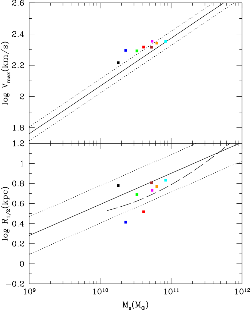
Figure 2.— Maximum circular velocity (top panel) and half-mass radius (lower panel) are plotted as a function of the galaxy stellar mass for our set of simulated galaxies (colored, solid squares). The color-code setting is the same as in Figure 1. The mean $V_{\rm max}-\mbox{$M_{s}$}$ (Tully-Fisher) and $R_{1/2}$–$M_{s}$ correlations inferred from observations by Avila-Reese et al. (2008) are shown as solid lines. The dotted lines encompass the estimated 1$\sigma$ intrinsic scatter. The dashed line in the lower panel is a more recent determination of the $R_{1/2}$–$M_{s}$ relation of late-type galaxies for a large SDSS sample by Bernardi et al. (2014).

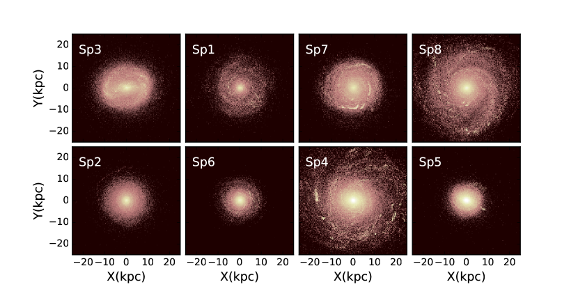
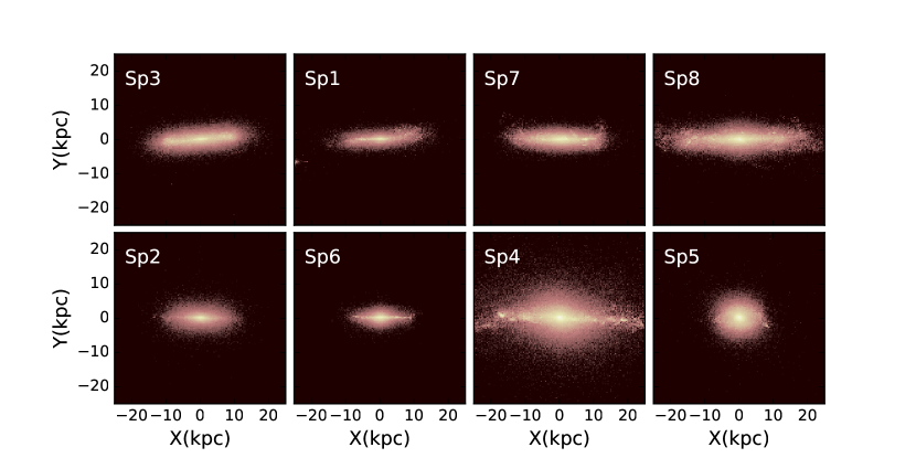
Figure 3.— Luminosity surface density in the R band in $L_{\odot}/\mbox{kpc}^{2}$ units for the eight runs sorted from highest to lowest values of $D/T$. The scale of colors goes from 5 to 7.2 in the log, the lighter the color the higher the luminosity. Top panels show a face-on view of the galaxies while bottom panels show the edge-on view.

In Figure 1, we depict the circular velocity curves $\sqrt{GM(<r)/r}$, as a proxy for $V_{\rm rot}$, for our entire set of runs. The color setting is shown inside the panel and will remain so for other figures unless otherwise stated. In agreement with the results of Roca-Fàbrega et al. (2016), our curves are also nearly flat. We see, however, some differences among the runs. For instance, Sp1 shows a gently rising inner part and ends up with the lowest $V_{\rm max}$ value; moreover, Sp7 has a $V_{c}$ curve similar to that of the MW. At the solar radius, $V_{c}$ is 224 km/s close to the value accepted for the rotation velocity of the Galaxy (e.g., Koposov et al., 2010). It is interesting to note that although the $V_{c}$ curves of runs Sp5 and Sp6 are very similar (they are slightly peaked), the former does not show a stellar disk (see Figure 3 below) whereas Sp6 does. One then needs to be cautious when trying to infer the presence of a disk by just looking at the shape of the circular velocity curve.

In the upper panel of Figure 2, we plot the $V_{\rm max}$ values, shown in Table 1, against $M_{s}$ (colored, solid squares). The color-code of the runs is the same as in Figure 1. The solid black line is the best orthogonal fit to a compilation and homogenization of observations by Avila-Reese et al. (2008); the masses were corrected by -0.1 dex to pass from a diet-Salpeter IMF to a Chabrier one. The dotted lines show the intrinsic scatter ($1\sigma$) reported in that work. In general, the simulated galaxies follow the observed stellar Tully-Fisher relation. In a more detailed comparison, we see that three of the disk-dominated runs lie above the $1\sigma$ intrinsic scatter, with a shift of $\approx 0.07$ dex in $\log V_{\rm max}$ from the mean relation. In the case of the spheroid-dominated galaxies, they are expected to have higher values of $V_{\rm max}$ than the disk-dominated ones. Other authors have also found, for their simulated MW-sized galaxies, a slight shift in the Tully-Fisher relation towards the high velocity side (c.f. Guedes et al., 2011; Aumer et al., 2013; Marinacci et al., 2014; Murante et al, 2015). However, biases in the selection process of simulated systems with respect to the observed galaxy samples, as well as differences between the observational measures and those performed here, unable us to claim whether there is a potential problem or not.

In the lower panel of Figure 2, $R_{1/2}$ against $M_{s}$ is shown for the eight runs (colored, solid squares). The solid and dotted lines are the linear fit (in logarithmic scales) to the same galaxy sample used in Avila-Reese et al. (2008) for determining the Tully-Fisher relation. These authors present the galaxy scale radius, so we multiply by a factor of 1.68 to pass to $R_{1/2}$. We also show in Figure 2 the mean $R_{1/2}$–$M_{s}$ relation as inferred in Bernardi et al. (2014) for a large sample of late-type SDSS galaxies and after a careful two-component photometric decomposition of them; their analysis is only for galaxies more massive than $10^{10}$ $M_{\odot}$. In general, we see that our simulated galaxies are in good agreement with the local $R_{1/2}$–$M_{s}$ correlation from observations. The two runs that deviate most, Sp5 (red) and Sp6 (blue), are spheroid-dominated galaxies. Observations show that early-type galaxy have indeed smaller effective radii than late-type ones (see e.g., Bernardi et al., 2014).

3.2. Morphology

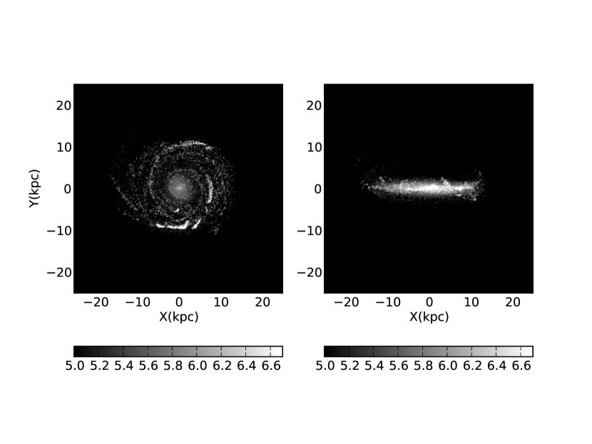
Figure 4.— Luminosity surface densities in the U band in $L_{\odot}/\mbox{kpc}^{2}$ units for run Sp7. As the U band samples young stellar populations, this figure is representative of the places in the galaxy where SF is going on. The U band traces better the spiral arms and the thin disk than the R band (compare this figure with the panels corresponding to Sp7 in Fig. 3

.

Figure 5.— Distribution of the mass-weighted stellar circularities $\epsilon$ for our sample of galaxies at $z=0$. We have considered only the stellar particles inside the sphere with radius 0.1$R_{\rm vir}$ and have used the definition by Scannapieco et al. (2009) in the computation of $j_{c}$, the specific angular momentum of a reference circular orbit. As expected from the $D/T$ (or $f_{disk}$ values) values of Table 1 and previous discussion on morphology, we see that the component associated with the disk of runs Sp4 and Sp5 do not contribute much to the stellar mass of the galaxy. Sp2 and Sp6, moreover, are intermediate cases.

In Fig. 3, we show the spatial luminosity distributions in the R band (proportional to the stellar mass distribution) for our eight simulated galaxies at $z=0$, both in face-on and edge-on projections. The luminosity surface density grid was constructed by using the publicly available stellar evolution code CMD2.7 (Marigo et al., 2008), assuming solar metallicity. All images use the same logarithmic scale which goes from 5.0 to 7.2 in solar luminosities per kpc² and cover the same physical extension of 50 kpc of side. At any epoch, in particular at $z=0$, the plane of the disk, and thus the face-on orientation, is defined by the angular momentum of the cold gas inside a sphere of radius $\sim 5$ kpc/h comoving. We check that the plane orientation is not sensitive to the value of this radius.

Galaxies in Fig. 3 are ranked by their $D/T$ values, in face or edge-on, from the highest (left, upper panel) to lowest (right, lower panel). The first four galaxies have $D/T>0.5$: they show relatively flat disks with well defined spiral structures. Runs Sp2 and Sp6 have very thick disks and no clear evidence of spiral structures. The two runs with the smallest $D/T$ values are Sp4 and Sp5. The former, while in its edge-on projection shows an oblate structure, in the face-on projection reveals well defined spiral structures. As will be shown below, this galaxy is assembled relatively late and had a recent merger and a burst of SF ($\sim 3-4$ Gyr ago); it seems that, as long as there is gas in the colliding galaxy, a thin disk with SF and spiral structure can be formed after the merger. The run Sp5, as discussed above, has a violent early and late-assembly history that has impeded it to form a disk component at any epoch; at $z=0$, its kinematic disk-to-total ratio is only 0.1 (see Table 1). This is compatible with what is seen in Figure 3, that is an spheroidal structure. Finally, note that in none of the runs the presence of a clear bar at $z=0$ is observed. A similar result was reported by Aumer et al. (2014). We will study this question in detail elsewhere.

In Figure 4, we show the U band face-on and edge-on projections of run Sp7. The U band projection is color-coded in grey and its color bar goes from 5 to 6.7 in the log in units of $L_{\odot}/\mbox{kpc}^{2}$. This band samples much better the young stellar population which, as can be appreciated in the figure, resides in a thin disk and spiral arms.

To distinguish the spheroid from the stellar disk using kinematics, it is usual to compute the probability distribution function of the stellar circularity $\epsilon$. This is defined as the ratio between the component of the specific angular momentum perpendicular to the plane of the disk $j_{z}$ to the specific angular momentum of a circular orbit at the stellar particle position $j_{c}$ (Scannapieco et al., 2009). This latter is computed as $j_{c}=rV_{c}(r)=r\sqrt{\mbox{G}M(<r)/r}$, where $r$ is the distance of the particle to the center and $M(<r)$ is the total mass inside $r$. A second definition is also often used in which the previous formula for $j_{c}$ is substituted by the maximum specific angular momentum the particle can have given its binding energy $E$. In the second case $\epsilon$ is always $\leq 1$. We will use the first definition because in this case $j_{c}$ is straightforward to compute.

In Table 1, we present two estimates of the kinematic disk-to-total ratio of our runs: $D/T=(T-B)/T$, where $T$ is the stellar mass in the galaxy and $B$ is the stellar mass of the spheroid, defined as twice the stellar mass found in the counterrotating galaxy stellar component (Abadi et al., 2003; Colín et al., 2010), and $f_{\rm disk}=M_{s}(\epsilon>0.5)/\mbox{$M_{s}$}$. Although both estimates give similar results, we see that for Sp1, Sp3 and, to a lesser degree for Sp2 and Sp7, the $D/T$ value is higher than the $f_{disk}$ one. This difference could be explained if there is a component with positive but low circularity values, that are thus not considered in the $f_{\rm disk}$ counting. Figure 5 show that this is actually the case: there is an excess on the low-$\epsilon$ part of the symmetric disk distribution that peaks around $\epsilon=0.9$. As anticipated from the reading of the $D/T$ and $f_{\rm disk}$ columns in Table 1 and from Fig. 3, runs Sp1, Sp3, Sp7 and Sp8, are clearly examples of disk galaxies; they have $D/T$ values close to those found by Marinacci et al. (2014) for their Aquarium halos (see their Figure 4, square brackets). For their two galaxies, GA2 and AqC5, Murante et al (2015) found $D/T=0.8$ and 0.77, respectively, similar to the values of our Sp3 (0.81) and Sp1 (0.75) runs. The runs Sp2 and Sp6 present a disk but it is not dominant, while runs Sp4 and Sp5 are by far spheroid-dominated galaxies.

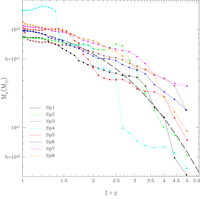
Figure 6.— Mass assembly histories of our suite of simulations. In the Y axis is plotted the total mass: the sum of the masses of the DM, stellar, and gas components, all inside the current virial radius. We see that Sp4 (cyan) and Sp5 (red) have had recent major mergers. The median assembly history reported in Rodriguez-Puebla et al. (2016) for $\mbox{$M_{\rm vir}$}(z=0)\approx 10^{12}\ \mbox{$M_{\odot}$}$ halos is shown as a black dashed line.

3.3. Mass assembly histories

The halos were selected to be at $z=0$ in relative isolation. Can they all be expected to harbor a galaxy with a significant disk component? Not necessarily. It is known that the stellar contribution of this component is more strongly related rather to the halo mass aggregation histories (MAHs) (see e.g., Scannapieco et al., 2015). In Figure 6 we depict the (total) MAHs of our suite of simulations. For comparison, the median MAH reported in Rodriguez-Puebla et al. (2016) for $\mbox{$M_{\rm vir}$}(z=0)=10^{12}\ \mbox{$M_{\odot}$}$ halos from several N-body large cosmological simulations is also plotted (black dashed line).

Two of the runs, Sp4 (cyan) and Sp5 (red; see Table 1), have a late violent assembly history, acquiring half of their present-day masses at $\mbox{$z_{half}$}\simeq 0.48$ and 0.9, respectively. Sp5 actually increases its mass by about a factor of 2.5 from $z=1$ to 0.4, and Sp4 have a major merger, quite visible in the figure, around $z=0.4$. The galaxies formed in these two halos are those with the lowest $D/T$ ratios, being completely spheroid-dominated. The run Sp2, which presents a significant spheroid component ($D/T=0.43$), had a significant merger at $z\sim 1.9$ and after that the mass increased very little. Aside from these runs, the rest have more quiet late halo MAHs, forming half of its mass at $z>1$; for example, $\mbox{$z_{half}$}\simeq 1.5$ for Sp8, a disk-dominated galaxy with a very regular stellar mass assembly history.

In summary, we see that the halo MAH has a relevant effect on the galaxy morphology. However, we have also a case where the formation of a prominent spheroid seems not to be related to the MAH of the system, namely run Sp6 ($D/T=0.30$). This run presents a very regular halo MAH, actually without major mergers at any epoch but with an early assembly of mass; its SFR decayed long ago. Cases of spheroid formation in simulated MW-sized galaxies, not related to the halo MAH, were reported and discussed previously, for instance, in Sales et al. (2012) and Aumer et al. (2014). These authors find that slowly rotating spheroids can form in systems where the angular momentum of the infalling gas is misaligned and the gas is accreted directly through cold filaments; these events are likely to be major contributors to the central mass growth of the galaxy.

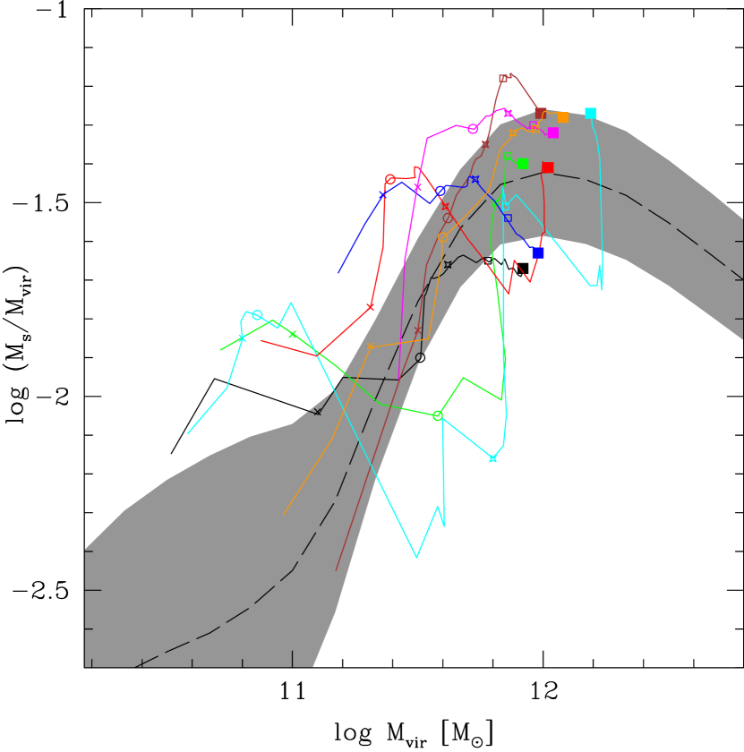
Figure 7.— Evolution of the stellar-to-halo mass fraction plotted against the halo (total) mass for our suite of runs. With solid squares, empty squares, four pointed stars, circles, and crosses are shown the values at $z=0$, 0.54, 1.0, 2.07, and 3, respectively. The trajectories begin at $z=4$. The color-code is the same as in previous figures. The gray shaded area and the dashed line are the $1\sigma$ intrinsic scatter and the mean, respectively, inferred for $z\sim 0$ central galaxies in Rodríguez-Puebla et al. (2015) It is interesting to see that the disk-dominated simulated galaxies move in this plot nearly along the $z\sim 0$ stellar-to-halo mass relation.

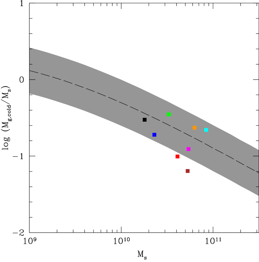
Figure 8.— The ratio of cold gas to stellar mass plotted as function of this latter. As in Figure 2, with colored squares we show the predicted values by our set of runs. The shaded area and the dashed line are the 1$\sigma$ intrinsic scatter and its mean, respectively, from the observational compilation and homogenization by Calette et al. (2016) for late-type galaxies.

3.4. Stellar and Gas fractions

In Figure 7, the stellar-to-halo mass fraction, $M_{s}$/$M_{\rm vir}$, as a function of $M_{\rm vir}$ for our set of runs are plotted. The $\mbox{$M_{s}$}/\mbox{$M_{\rm vir}$}$ values at $z=0$ are shown as solid squares. The gray shaded area ($1\sigma$ error bars) is from the accurate semi-empirical determinations at $z\sim 0$ by Rodríguez-Puebla et al. (2015) for central galaxies (satellite galaxies present a slightly different $M_{s}$–$M_{\rm vir}$ relation). Our simulated MW-sized galaxies are consistent with the semi-empirical determinations.

In Figure 7, we also depict with color lines the evolutionary tracks of the runs in the $M_{s}$/$M_{\rm vir}$–$M_{\rm vir}$ plane. We show five redshifts along the tracks, $z=0,0.5,1,2,3,$ and 4 (solid squares, empty squares, stars, circles, crosses, and the end of the lines, respectively). Interestingly enough, the most disky runs (Sp1, Sp3, Sp7, and Sp8) evolve nearly along the semi-empirical $z=0$ $M_{s}$–$M_{\rm vir}$ correlation, specially Sp3 and Sp8. The two most spheroid-dominated runs (Sp4, cyan line, and Sp5, red line) present very irregular evolutionary tracks, likely due to the major mergers they suffer. In general, the fact that the $M_{s}$/$M_{\rm vir}$ evolutionary tracks of the simulated galaxies do not deviate significantly from the $z=0$ $M_{s}$/$M_{\rm vir}$–$M_{\rm vir}$ correlation, at least up to $z\sim 2$, would imply that this correlation does not evolve significantly in the $10^{11}-10^{12}$ halo mass range.

In Figure 8, the cold gas-to-stellar mass ratio, $M_{g,cold}$/$M_{s}$, as a function of $M_{s}$ are plotted for the eight runs. They are compared to the correlation inferred from an extensive compilation and homogenization of observations for local late-type galaxies (Calette et al., 2016, gray band, corresponding to 1$\sigma$ intrinsic scatter). We see that most runs are within the 1$\sigma$ intrinsic scatter of the observational correlation. Those that deviate most are run Sp5, a spheroid-dominated galaxy with the lowest $D/T$ value of our sample (only 0.1), and run Sp3, a disk galaxy with actually the highest $D/T$ value. As we will see below, Sp3 had a second and long period of very active SF that likely reduced the amount of cold gas at present-day, with respect to the other disk galaxies. The footprint of this second burst of SF and deficit in cold gas can also bee seen in its stellar-to-halo mass fraction; the Sp3 galaxy has the second highest value of $M_{s}$/$M_{\rm vir}$ among all runs (see Figure 7).

An interesting question is what are the fractions of the different baryonic components inside the virial radii of our MW-sized simulated galaxy/halo systems. In the case of stars and cold gas, at $z=0$, they are located practically only within the central galaxies. The average and standard deviation of the $M_{s}$/$M_{\rm vir}$ fraction normalized to the the universal baryonic mass fraction, $f_{s}=\mbox{$M_{s}$}/\mbox{$M_{\rm vir}$}/f_{\rm univ}$ ($f_{\rm univ}\equiv\Omega_{b}/\Omega_{m}=0.15$ for our cosmology), from our eight simulations are $\langle f_{s}\rangle=0.2775\pm 0.1039$. For the cold gas, $\langle f_{\rm cold}\rangle=0.0536\pm 0.0275$, that is the cold gas mass is $\sim 1/5$ of the stellar mass, and both account for approximately one third of the universal baryonic fraction inside the virial radius of the halos. Where are the remaining baryons? A similar exercise was done but now for the cool ($10^{4}<T/K\leq 10^{5}$), warm-hot ($10^{5}<T/K\leq 10^{7}$) and hot ($T>10^{7}K$) gas. Most of the mass of these gas components are located outside the galaxies, in the circum-galactic medium (CGM). The average and standard deviations of the corresponding fractions (within 1$R_{\rm vir}$) are: $\langle f_{\rm cool}\rangle=0.0343\pm 0.0283$, $\langle f_{\rm w-h}\rangle=0.2425\pm 0.0790$, $\langle f_{\rm hot}\rangle=2.7\times 10^{-6}\pm 4.3\times 10^{-6}$. The sum of all of these baryonic components does not account for the universal baryonic fraction. The missing mass is $0.3925\pm 0.1388$. Therefore, $\approx 25-53\%$ of the baryons in our MW-sized simulations resides outside the corresponding virial radii.

Recently, Wang et al. (2016) have reported the baryonic fractions mentioned above for their 88 simulated galaxies, which cover a large range of masses (the NIHAO project). The average values reported for their systems in the $0.3-3.5\times 10^{12}$ $M_{\odot}$ halo mass range, roughly agree with those found here, though we predict a smaller fraction of cool gas ($\langle f_{\rm cool}\rangle=0.034$ vs. 0.109) and a higher fraction of warm-hot gas ($\langle f_{\rm w-h}\rangle=0.242$ vs. 0.167) than Wang et al. (2016). These differences could partly be due to the fact that their averages include systems less massive than ours and, as they show, $f_{\rm cool}$ decreases and $f_{\rm w-h}$ increases for massive systems. Following Wang et al. (2016), we can compare the different gas fractions in the CGM with recent observational constraints for the MW and $L^{*}$ galaxies using quasar absorption lines (Werk et al., 2014, see more references therein). According to the latter authors, over $25\%$ of the baryon budget is accounted for by cool, photo ionized gas in the CGM. This is $\sim 7\times$ higher than the mean fraction measured in our simulations. On the other hand, the fraction of warm-hot gas in our simulations is higher than conservative observational estimates (e.g., Peeples et al., 2014, $24\%$ vs. $5\%$) and well within the range of less conservative estimates. Finally, both our simulations and observations, show that the fraction of hot gas is very small, though in our case is much smaller than estimates from $X-$ray observations. As in Wang et al. (2016), we conclude that while the total gas fraction measured in our simulations ($\approx 35\%$ on average) seems to be consistent with the observational estimates in $L^{*}$ galaxies, the mix of temperatures in the CGM strongly disagrees with current observational estimates.

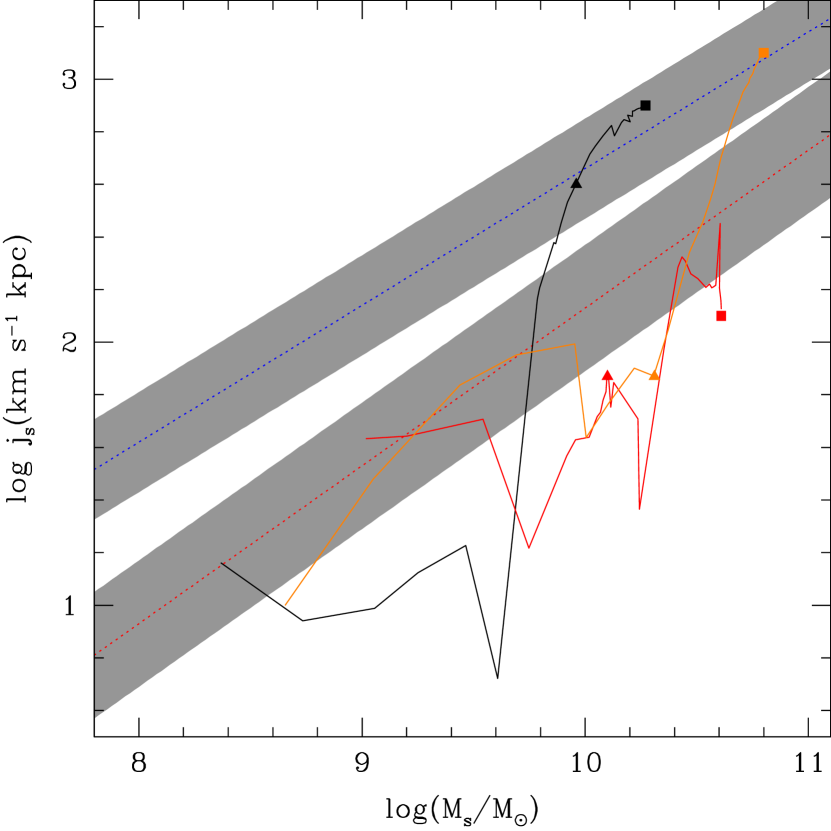
Figure 9.— Evolution of the specific stellar angular momentum $j_{s}$ plotted against the stellar mass for three of our runs: Sp1, Sp5, and Sp8. Color code is as in Figure 6. Straight dotted lines are fits from Romanowsky & Fall (2012), red is for elliptical and blue for spiral galaxies. The curves are plotted from $z=4$ to present-day, this latter shown with solid, colored squares. The points at $\sim\mbox{$z_{half}$}$ have highlighted with solid triangles.

3.5. Evolution of angular momentum

We compute the evolution of the stellar specific angular momentum, $j_{s}$, for our suite of simulations and plot it as a function of the galaxy stellar mass in Figure 9. For clarity, only the evolution of runs Sp1 and Sp8, two disk-dominated galaxies, and Sp5, a spheroid-dominated galaxy, are shown. Lines start at $z=4$, low $j_{s}$ values, and end at $z=0$, shown in solid squares. We highlight with solid triangles the epochs at which runs reach half of their stellar mass. The straight dotted lines are observation-based fits from Romanowsky & Fall (2012); the blue one is for spirals while the red one is for ellipticals. The shaded area show the 1$\sigma$ scatter.

We found that all runs have low $j_{s}$ values at early times. This is in line with the finding by Agertz & Kravtsov (2015). They report similar values, although, depending on the strength of the feedback, they fluctuate more or less. Consistent with the $D/$T values shown in Table 1, the Sp1 and Sp8 galaxies end up in the spiral region while the Sp5 galaxy never leaves the elliptical zone and it actually ends up below it. On the other hand, its late ($z<\mbox{$z_{half}$}$) strongly fluctuating $j_{s}$ history is consistent with the fact that more than half of its mass is assembled at $z<1$. We see that disky Sp1 and Sp8 runs (and also Sp3 and Sp7, not shown) have a smooth late evolution in which $j_{s}$ increases all the time. They differ each other on when this smooth period of angular momentum growth begins; for example, for Sp1 it happens at $z\sim 1.8$, a little later (0.7 Gyr) after the last major merger (LMM), while for Sp8 we can identify it at $z\sim 1.3$, 2 Gyr after the LMM. The spheroid-dominated Sp5 (as well as Sp4 and Sp6) runs have an episodic evolution of $j_{s}$ but most of time their $j_{s}$ values are below or within the region inferred from observations for local early-type galaxies.

3.6. Star formation history

Aside from Sp2, all runs, even those with a massive spheroid component, show present-day SFRs (see Table 1) that are comparable to those of late-type spiral galaxies at $z=0$ (c.f. Schiminovich et al., 2007). In particular, the most rotational supported disks have values close or even higher than those reported for the MW (e.g., Robitaille & Whitney, 2010), consistent with the gas fractions predicted for these runs. In Figure 10 we show the “archaeological” SF history (SFH) for our set of runs. This is determined from the snapshot at $z=0$ by simply counting the mass in stellar particles in a given age (time) bin and divided it by the width of the bin. We divide the time since Big Bang in bins of 0.5 Gyr. Thus, in each panel, in the left (right) we have the oldest (youngest) stellar particles.

In agreement with the many SFHs shown in works on the subject (e.g., Governato et al., 2004; Guedes et al., 2011; Hummels & Bryan, 2012; Murante et al, 2015), we also see in all of our runs (but Sp4) the characteristic early peak of SF, registered in the violent phase of halo mass assembly. The strength and duration of the “burst” vary with the run. Somehow unexpected, in the most disky runs (with the highest kinematic $D/T$ values), one sees a second peak of SF located in time well after the LMM, during the smooth growth phase of the angular momentum. Regarding the most spheroid dominated galaxies, Sp4 (cyan) and Sp5 (red), they show relatively strong SF activity in the last few Gyr as the result of their late mergers. Thus, the origin of spheroid-dominated MW-sized galaxies in a relatively isolated environment can be related in some cases to late mergers with significant fractions of gas and ulterior bursts of (recent) SF. Therefore, one expects that a fraction of MW-sized early-type galaxies in the field have a different structure and stellar population composition as compared to cluster early-type galaxies of similar masses.

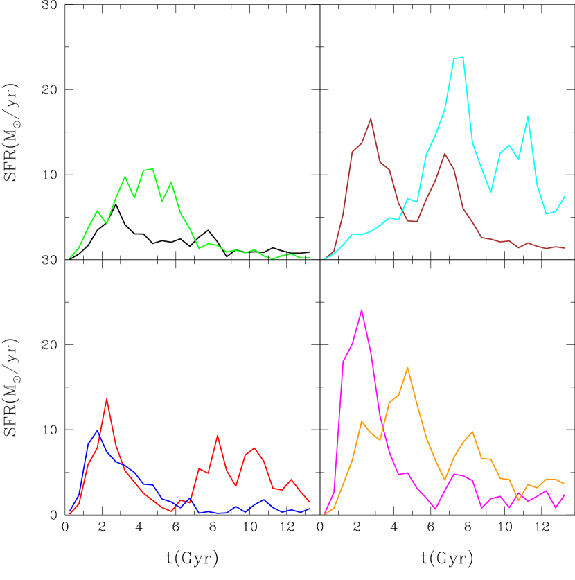
Figure 10.— Star formation rate, measured as a stellar age histogram, as a function of cosmic time, in bins of 0.5 Gyr width, for all the eight runs. We place in each panel two runs and they are color-coded as in Figure 6; for example, Sp1 (black line) and Sp2 (green line) are in the top left panel, and Sp7 (magenta line) and Sp8 (orange line) are in the bottom right one. All runs show a prominent first peak, related to the violent phase of the assembly history. The disk-dominated runs Sp1, Sp3, Sp7 and Sp8 also present a second peak, produced well after the last major merger, during the smooth growth of the angular momentum.

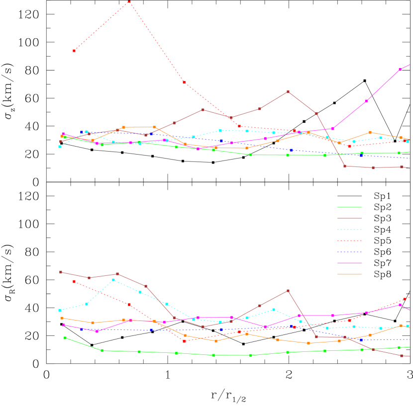
Figure 11.— Azimutally-averaged velocity dispersions in the vertical (upper panel) and radial (lower panel) directions for the runs with $D/T>0.4$ at $z=0$, Sp1, Sp2, Sp3, Sp7, and Sp8 (solid lines) and those with $D/T\leq 0.4$, Sp4, Sp5, and Sp6 (dotted lines).

3.7. Gas velocity dispersions

A relevant ISM property is the cold gas velocity dispersion. The large-scale SF of disk galaxies could proceed by a self-regulation mechanism in the ISM driven by the balance between the injected (by SNe) and dissipated kinetic energy in the ISM (e.g., Firmani & Tutukov, 1992; Avila-Reese & Firmani, 2000; Tamburro et al., 2009; Klessen & Hennebelle, 2010). In this context, the cold gas velocity dispersion is directly related to the SN-driven feedback. We will discuss this self-regulation model in the light of our simulations in subsection 4.5.

In Fig. 11, we present the gas surface density-weighted velocity dispersion profiles of the simulated galaxies at $z=0$ for both the radial and vertical components, $\sigma_{r}$ and $\sigma_{z}$, respectively. Only gas cells with $T<10^{4}$ K and $|z|\leq 1$ kpc, where $z$ in this case is the $z$ coordinate, perpendicular to the plane, are taken into account. The runs with $D/T>0.4$, Sp1, Sp2, Sp3, Sp7, and Sp8, are shown with solid lines while those with $D/T\leq 0.4$, Sp4, Sp5, and Sp6 are shown with dotted lines.

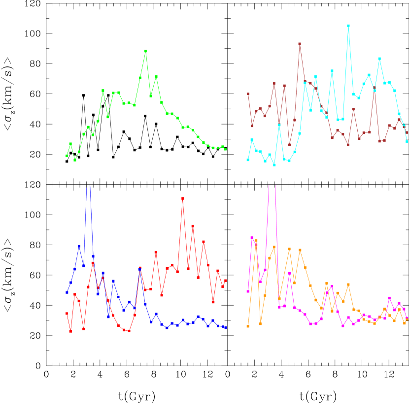
Figure 12.— Evolution of the mean surface density-weighted vertical velocity dispersions of the eight simulated galaxies.

The gas velocity dispersion is moderately anisotropic, more for the spheroid-dominated galaxies. The $\sigma_{z}$ profiles are nearly flat with values mostly around 25-35 km/s up to $\sim 1.5\mbox{$R_{1/2}$}$, except for Sp5. The latter galaxy had recent mergers and strong bursts of SF; therefore, the small fraction of remaining cold gas is still strongly turbulent. In several cases, $\sigma_{z}$ increases with radius in the outermost regions, above 1–1.5 $R_{1/2}$. The radial velocity dispersion profiles, $\sigma_{r}$($r$), are also nearly flat for the disk-dominated galaxies (with values around 15-30 km/s) and with higher values in the inner regions for the Sp5 and Sp6 runs, which are spheroid-dominated galaxies that suffered relatively recent mergers. The Sp3 run, while disk-dominated, presents large values of $\sigma_{r}$ in the inner disk and increasing values of $\sigma_{z}$ in the outer disk; the gas of this galaxy is being perturbed by a relatively massive ($M_{s}\sim 10^{10}\ \mbox{$M_{\odot}$}$) satellite that is inside $R_{\rm vir}$ at $z=0$.

The observational measure of the cold (HI and/or CO) gas velocity dispersion profiles in galaxies is not an easy task. For data cubes, the gas velocity dispersion is calculated from the second-moment map. For example, in Tamburro et al. (2009) the data cubes of 11 galaxies from the “The HI Nearby Galaxy Survey” (THINGS; Walter et al., 2008) are used to calculate the line-of-sight (intensity-weighted) velocity dispersion at each pixel. In Mogotsi et al. (2016, see also , ), the line-of-sight (natural-weighted) velocity dispersion is calculated from Gaussian fits to the line profiles. These authors studied both the THINGS HI and the “HERA CO Line Extragalactic Survey” (HERACLES) CO line profiles of 13 galaxies; they present results also using the second moments of the HI profiles.

For spiral MW-sized galaxies, the mentioned above observational results show line-of-sight velocity dispersions that mostly decrease with radius. For most cases, the velocity dispersion profiles flatten in the outer regions, attaining values around $10$ km/s. The mean/median values of the line-of-sight velocity dispersion of observed galaxies range from $\approx 8$ to 20 km/s, which are up to $\sim 1.5$ times lower than the mean surface density-weighted vertical and radial velocity dispersions of our simulated galaxies, $\langle\sigma_{z}\rangle$ and $\langle\sigma_{r}\rangle$, respectively. It is difficult to conclude whether there is a disagreement or not between simulations and observations, because of the large differences in the way of measuring the velocity dispersions among different observational studies and the likely biased way simulations of comparing simulations with observations. Within this level of uncertainty, we can just say that the velocity dispersion profiles in our simulations are not in strong conflict with those inferred from different observational studies. This implies that we are in the limit of the stellar feedback efficiency because the cold gas velocity dispersion (and gas disk thickness) significantly increase with this efficiency (see Marasco et al., 2015).

In Fig. 12, the evolution of $\langle\sigma_{z}\rangle$ is shown for the eight MW-sized runs. By comparing this plot with figure 10, we see a trend of the $\langle\sigma_{z}\rangle$ history to roughly follow the global SF history. In general, the velocity dispersions of the simulated galaxies are larger at higher redshifts, when the galaxies are having frequent mergers and strong bursts of SF. Recent observational inferences of CO velocity dispersions in high redshift galaxies, show that they are indeed characterized by clumpy gaseous disks much more turbulent than the local ones. The measured velocity dispersions of star forming galaxies at $z\sim$1–3 are close to their rotation velocities, unlike in local galaxies, where the former velocities are much lower than the latter ones (e.g., Law et al., 2007, 2009; Förster Schreiber et al., 2009; Epinat et al., 2012; Lehnert et al., 2013).

4. Discussion

4.1. Resolution issue

In Roca-Fàbrega et al. (2016), they compared their results from the high resolution simulation G.321 ($7\times 10^{6}$ DM particles inside $R_{\rm vir}$ and 109 pc of resolution) with the ones from G.321_lr, a simulation with twice less resolution and about eight times less DM particles, and found good convergence except for the SFR and the amount of cold gas(the comparison is only made at $z=0$). For the former, they report 0.27 $M_{\odot}$/yr for G.321 against 0.16 for G.321_lr, a factor of 1.7 higher for the high resolution run. For the latter, a higher difference is found, $9.3\times 10^{9}\mbox{$M_{\odot}$}$ for G.321 against $1.4\times 10^{9}$ for G.321_lr. Guided by these results and the resolution study of Scannapieco et al. (2012), we run again the Sp7 galaxy but with one less level and eight times less DM particles. For this low resolution simulation, the values of the total, stellar, and cold gas mass inside the galaxy are: $1.06\times 10^{12}$, $5.05\times 10^{10}$, and $3.76\times 10^{9}\ \mbox{$M_{\odot}$}$, respectively. Such values differ from the corresponding ones in the higher resolution simulation by 2.7%, 3.6%, and 41%, respectively (see Table 1). Moreover, the $V_{\rm max}$ value differ by less than 1%. Overall, we see that for global and cumulative quantities, like the stellar mass, good convergence is achieved. On the other hand, we have found in the low resolution simulation a lower present-day SFR and lower specific angular momentum. The values are: (SFR/$M_{\odot}$ yr${}^{-1},j_{s}$/km s^-1 kpc)=(0.7,605). These are to be compared with (3.2,957), found for the higher resolution counterpart. That the $j_{s}$ value is lower in the low resolution run is not surprising because it is long known that $j_{s}$ does depend on resolution (Governato et al., 2004). Aside from the two-body heating and the dynamical friction effect of the halo on the accreting lumpy substructure, there is also the torque exerted by the halo on an asymmetric, not well resolved, disk (Mayer et al., 2008). It seems, however, that resolution through artificial loss of angular momentum is also the culprit of the lower SFRs and cold gas mass values reported above.

Have we reached convergence given our SF and feedback scheme and the corresponding chosen parameters? This is a question that could be addressed by running simulations with even more resolution. Unfortunately, this can not be performed with the present set of simulations, so we can only speculate. On the other hand, the experiment by Roca-Fàbrega et al. (2016) seems to suggest that $\sim\ 10^{6}$ DM particles and $\sim\ 220$ pc resolution are not enough, at least as the SFR and amount of cold gas is concerned. It is not clear, on the other hand, if the present stellar feedback scheme, considered in this and other related papers (see, for example, Roca-Fàbrega et al. (2016)), can be applied to much smaller scales ($\sim 50$ pc or below) because at these scales physical processes, such us the gas heating by ionizing radiation (e.g., Hopkins et al., 2014; Trujillo-Gomez et al., 2015) should be included. It is also possible that, because our stellar feedback is deterministic, convergence (for a given $\epsilon_{\rm SF}$ and $n_{\rm SF}$) may not be achieved since twice smaller cells (two times better resolution) would imply eight times less massive SPs on average. Thus, twice higher resolution means that the increase of temperature (to several $10^{7}\mbox{K}$) happens in only 1/8 of the cell of the less resolved simulation. This process could be non-linear and therefore convergence may not be guaranteed.

4.2. Star formation and stellar feedback

The present version of the (deterministic) SF and stellar feedback recipes have been used since the paper by Colín et al. (2010) (see also, e.g., Avila-Reese et al., 2011; González-Samaniego et al., 2014). In particular, the paper by Colín et al. (2010) focused on the impact of varying the SF and stellar feedback parameters on the properties of the simulated low-mass galaxies. For instance, it was seen that a lower $n_{\rm SF}$ produced a larger $R_{1/2}$ and a less peaked circular velocity. Moreover, because the thermal SNe energy is dumped into the target gas cell instantaneously, the lower $\epsilon_{\rm SF}$ the less efficient the feedback is. Unfortunately, because it is not implemented in the present version of the code, we can only speculate about what would happen if part of this energy were kinetic. It is interesting, on the other hand, to see that while this prescription produces a stellar-to-halo mass ratio of MW-sized galaxies that agrees with semi-empirical determinations, this is not the case for our simulated low-mass galaxies (see figure 6 of Avila-Reese et al., 2011).

4.3. “Explosive” feedback

In every cool and dense gas cell we let the code convert 65% of its mass into stars. This high fraction is really needed to overcome the overcooling problem. This spatial and time located injection of energy increase the temperature of the gas to several $10^{7}$ K degrees. This temperature is obtained by matching the expression for the internal energy of an ideal monoatomic gas with the energy injected by SNe associated with the stellar particle; that is, $T$ is given by

$$T=\frac{2}{3}\left(\frac{1}{Nk}\right)2\times 10^{51}N_{SNII},$$ (1)

where $N_{SNII}$ is the number of supernovae, which depends on the shape of the IMF and the mass of the stellar particle, and $N$ is the number of hydrogen atoms inside the cell where the SP was born. This latter is given by $n_{H}(1-\mbox{{$\epsilon_{\rm SF}$}})\Delta x^{3}$, where $\Delta x$ is the side of the cell, $n_{H}$ is the hydrogen number density which is greater but close to $n_{\rm SF}$, and $\mbox{{$\epsilon_{\rm SF}$}}=0.65$. We notice that this tempearture does not depend on the size of the cell because $N$ and $N_{SNII}$ both depend on $\Delta x^{3}$, the latter through the mass of the stellar particle. Since the gas density in the cell at the moment of SF is around $n_{\rm SF}$ (in our case 1 hydrogen atom per cubic centimeter), the gas pressure right after the SF event is huge, $10^{7}\ \mbox{K}\mbox{cm${}^{-3}$}$, clearly enough to overcome the external pressure and the negative “pressure” due to gravity (Ceverino & Klypin, 2009; Trujillo-Gomez et al., 2015). At these temperatures the crossing time is much smaller than the cooling time (Dalla Vecchia & Schaye, 2012) and thus, delaying the cooling after SF, to avoid the gas from radiating away most of its heat, becomes irrelevant. Yet, as the simulations in Roca-Fàbrega et al. (2016) were run assuming this delay in the cooling our simulations also consider this assumption.

4.4. Dark and baryonic mass assembly of MW-sized galaxies

Galaxies formed in halos of present-day masses $\mbox{$M_{\rm vir}$}\approx 10^{12}$ $M_{\odot}$ are in the peak of the $M_{s}$/$M_{\rm vir}$ correlation (see e.g., the gray area in Fig. 7); that is, galaxies of these masses were the most efficient in forming stars within their halos. As discussed in Subsection 3.4, our simulations are in rough agreement with the semi-empirical inferences of the $M_{s}$/$M_{\rm vir}$ correlation, and the most disk-dominated ones (Sp1,Sp3, Sp7, and Sp8) evolve closely along the $z=0$ $M_{s}$/$M_{\rm vir}$–$M_{\rm vir}$ correlation.

Is the $M_{s}$/$M_{\rm vir}$ evolution of our MW-sized galaxies consistent with look-back time semi-empirical inferences? In Fig. 13 (upper panel) we compare the $M_{s}$/$M_{\rm vir}$ tracks (solid lines) from the simulated galaxies with the average track for $\mbox{$M_{\rm vir}$}=10^{12}$ $M_{\odot}$ halos according to the inferences by Behroozi et al. (2013a, dashed line). Five of the simulated galaxies (those with the largest $D/T$ ratios) present a nearly constant value of the $M_{s}$/$M_{\rm vir}$ fraction since $\sim$6.5–10 Gyr ago, and then a fast decrease at earlier epochs. A similar behavior is seen for the average track inferred from the semi-empirical study. It is interesting to see that for MW-sized galaxies, both semi-empirical inferences and the simulations show that their stellar masses grow roughly as their halo masses during the last 6.5–10 Gyr (since $z\approx$ 0.7–2); at the earliest epochs, these galaxies were inefficient in forming stars (their $M_{s}$/$M_{\rm vir}$ fractions were below 1–3$\times 10^{-3}$) and then, at ages around 2–6 Gyr, when the initial burst of SF happens, the stellar mass grew up at a rate much faster than the halo mass, to finally enter in the quiescent regime in which $\mbox{$M_{s}$}(z)\propto\mbox{$M_{\rm vir}$}(z)$ roughly.

Aside from the fact that uncertainties in the determination of the $M_{s}$/$M_{\rm vir}$ correlation at high redshifts are large, the inferences by Behroozi et al. (2013a) shown in Fig. 13 suggest that galaxies formed in halos of present-day masses around $10^{12}$ $M_{\odot}$ assembled their stars later on average than our simulations. It is possible that at the early stages of galaxy formation, when the host halos were much less massive than today, the effects of early or preventive stellar feedback (see the Introduction for references) reduce significantly the SF. Moreover, we notice that the AGN-driven feedback is not yet implemented in the code. So, it could be that in our simple scheme too many stars are being formed in the earliest epochs. In any case, given the good agreement between observations and our simulated galaxies, there is not much room for other feedback effects, at least at the MW-sized scales studied here.

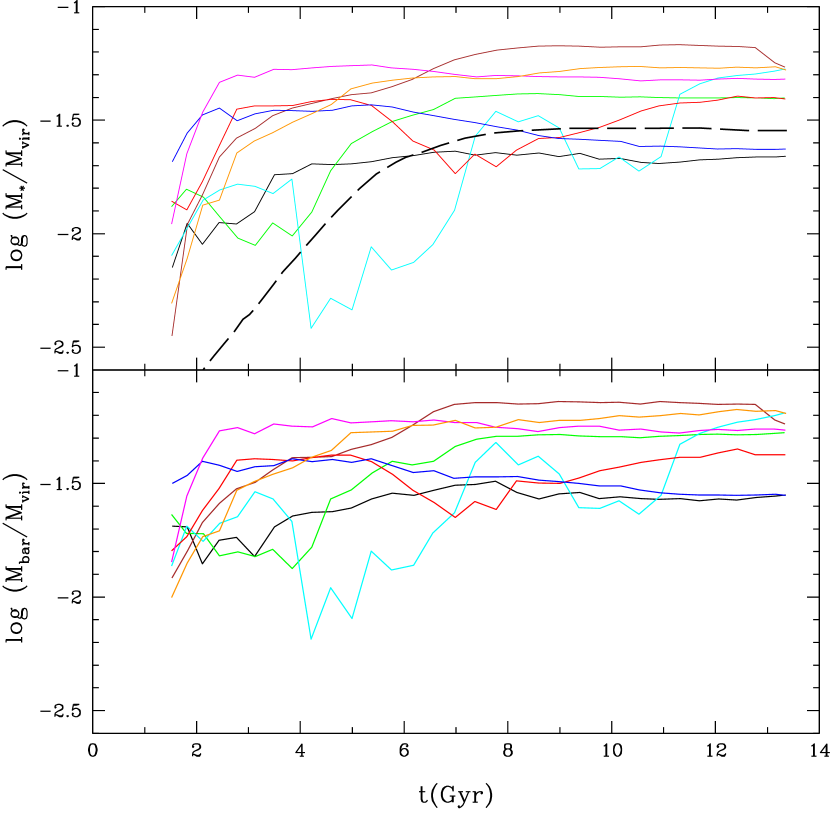
Figure 13.— Evolution of the $M_{s}$/$M_{\rm vir}$ (top panel) and $M_{b}/\mbox{$M_{\rm vir}$}$ (bottom panel) fractions for the eight runs. The color code is the same as in Fig. 1. The dashed line in the top panel is the average track for $z=0$ $\mbox{$M_{\rm vir}$}=10^{12}$ $M_{\odot}$ halos obtained from the look-back time semi-empirical inferences of Behroozi et al. (2013a).

It is interesting that the epochs at which the simulated galaxies reach the quiescent regime correspond roughly to the epochs where the halos attained a mass of $\approx 5\times 10^{11}$ $M_{\odot}$. Several semi-empirical studies have suggested that halos in the mass range $\mbox{$M_{\rm vir}$}\approx 0.5-1\times 10^{12}$ $M_{\odot}$ are those with the maximum SF efficiency at any epoch (e.g. Behroozi et al., 2013b; Lu et al., 2015). This can be explained as follows. The stellar feedback is able to blowout the gas from the galaxies with a efficiency that decreases as the gravitational potential gets stronger. Therefore, the more massive the galaxy/halo system is, the less gas is ejected due to stellar feedback. However, for halos above $\sim 10^{12}$ $M_{\odot}$, other astrophysical processes start to play an important role, making the efficiency of star formation to decrease with mass. These processes are the long radiative cooling time of the gas, shock heated during the virialization of massive halos (see e.g. Dutton et al., 2010), and the feedback of powerful AGNs, which appear at some evolutionary stages of massive galaxies (see for a review e.g., Somerville & Dave, 2015). The consequence of this is that galaxies evolving in halos with current masses of $\sim 0.5-1\times 10^{12}$ $M_{\odot}$ are expected to be the most efficient in capturing, keeping, and transforming gas into stars. For this reason, the stellar mass growth of these galaxies is expected also to be the less detached from the corresponding cosmological halo MAH. Nevertheless, even these systems with the highest efficiency of stellar mass growth, have $M_{s}$/$M_{\rm vir}$ values much lower than the universal baryonic fraction, $f_{\rm univ}\equiv\Omega_{b}/\Omega_{m}=0.15$ for our cosmology.

We can measure the baryonic mass of our simulated galaxies, $M_{b}=\mbox{$M_{s}$}+\mbox{$M_{g,cold}$}$, and calculate the galaxy baryonic fractions, $M_{b}/\mbox{$M_{\rm vir}$}$. The evolution of these fractions are plotted in the lower panel of Fig. 13. While the values of $M_{b}/\mbox{$M_{\rm vir}$}$ are larger than those of $M_{s}$/$M_{\rm vir}$, the former are still lower than $f_{\rm univ}$, at least by a factor of $\sim 3$ (see also Subsection 3.4). The $M_{b}/\mbox{$M_{\rm vir}$}$ evolutionary tracks are similar to the $M_{s}$/$M_{\rm vir}$ ones; nonetheless, at earlier epochs, there are somee differences which are related to the fact that the gas-to-stellar mass ratios increase with redshift.

As shown in Subsection 3.4, at $z=0$ a large fraction of baryons in the simulations are located actually outside the central galaxies, in the gaseous circumgalactic medium, in different phases (see also Sales et al., 2012; De Rossi et al., 2013; Roca-Fàbrega et al., 2016). We have found that on average $3.4\%$, 28.3%, and much lower than 1% of the universal baryon fraction is contained in cool, warm-hot, and hot gas in the halo (within $R_{\rm vir}$), respectively (for comparison, the mass fraction in stars in the simulated galaxies is on average $\approx 28\%$). Stellar feedback is presumably the culprit for keeping the gas in the halo in these phases. However, even taking into account these contributions, the baryonic budget within the virial radius of our simulations present an average deficit of $\approx 40\%$ with respect to $f_{\rm univ}$. Therefore, yet a significant fraction of baryons should be in form of gas at distances greater than virial radii. A detailed study of the origin and spatial distribution of the CGM in general will be presented elsewhere.

4.5. What does drive the gas velocity dispersion in galaxies?

Since MW-sized disk galaxies suffer less the influence of large-scale SN- and AGN-driven galactic winds, they are optimal to study whether the SF proceeds locally in a self-regulated way and whether the turbulent motions in the disks are driven by SN feedback or some other mechanisms. While the SF in the disk can be explained by the Toomre (Toomre, 1964) or generalized Toomre (Romeo & Wiegert, 2011) criteria, the physical conditions implied in these criteria are related namely to the SF and its feedback, as well as to properties of the turbulent ISM and the dynamics of the disk. In this context, one expects a self-regulated SF process controlled by ISM properties like the turbulence decay time, $t_{\rm d}$, or its porosity due to SN-remnant heated gas, as well as by the gas infall rate (e.g., Firmani & Tutukov, 1992; Silk, 1997; Klessen & Hennebelle, 2010).

A simple scheme of local self-regulated SF is the one based on the vertical balance between the rate of injected energy versus the dissipated kinetic one, which determines the gas disk height (Firmani & Tutukov, 1992, 1994; Avila-Reese & Firmani, 2000):

$$\mbox{$\gamma_{\rm in}$}\mbox{$\epsilon_{>8}$}\dot{\Sigma}_{*}(r)=\frac{\Sigma_{g}(r)\sigma_{z}^{2}(r)}{2t_{\rm d}},$$ (2)

where $\dot{\Sigma}_{*}$ and $\Sigma_{g}$ are the surface SF rate and neutral gas density, $\gamma_{\rm in}$ is the SN + Stellar Winds (from stars $>8\mbox{$M_{\odot}$}$) energy fraction that ends as kinetic energy in the ISM, and $\mbox{$\epsilon_{>8}$}=E_{\rm SN+Wind}\mbox{$\eta_{\rm>8}$}$ is the SN + Stellar Wind energy per unit of solar mass formed. In this equation, it is implicitly assumed that the gas velocity dispersion is driven only by SN + Wind feedback. We calculate $\sigma_{z}$($r$) from our simulation results by using the measured radial profiles $\dot{\Sigma}_{*}$($r$) and $\Sigma_{g}$($r$) (for the neutral, $T<10^{4}$ K, gas), and compare the obtained $\sigma_{z}$($r$) profiles with those measured. For this, we use the same value of $\epsilon_{>8}$ as in the simulations ($E_{\rm SN+Wind}=2\times 10^{51}$ erg and $\mbox{$\eta_{\rm>8}$}=7.5\times 10^{-3}$ $\mbox{$M_{\odot}$}^{-1}$ for a Miller-Scalo IMF). For $\gamma_{\rm in}$, the analytical solution of the SN-remnant evolution shows that it is equal to $\sigma_{z}/v_{w}$, where the terminal wind velocity is $v_{w}=340$ km/s (Spitzer, 1978). Numerical simulations of SN-remnant evolution have shown that $\mbox{$\gamma_{\rm in}$}\approx 0.1$ (Thornton et al., 1998), close to the analytical solution when the ISM velocity dispersion is 25-40 km/s, as in our simulations at $z\sim 0$. Observational inferences agree also with vales of $\mbox{$\gamma_{\rm in}$}\approx 0.1$ (Tamburro et al., 2009). We will use $\mbox{$\gamma_{\rm in}$}=\sigma_{z}/v_{w}$. For the turbulence decay, several numerical studies have demonstrated that supersonic turbulence dissipates rapidly, in a timescale roughly equivalent to the crossing time for the driving scale at the turbulence velocity (e.g., Mac Low, 1999; Stone et al., 1999; Avila-Reese & Vázquez-Semadeni, 2001). The latter authors have found values of $t_{d}\approx 15-20$ Myr for ISM properties typical of the MW. Here, we will assume a constant $t_{d}$ equal to $15$ Myr.

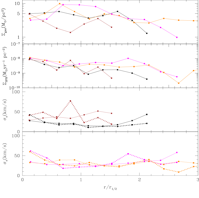
Figure 14.— Upper panels: Gas surface density and surface SF rate profiles at $z\sim 0$ for the disk-dominated runs (Sp1, Sp3, Sp7, and Sp8). The color code is the same as in Fig. 1. Lower panels: Gas vertical velocity dispersion profiles as measured for the same runs shown in the upper panels (solid lines) compared to the profiles calculated from $\Sigma_{g}$ and $\dot{\Sigma}_{*}$ profiles according to Equation 2 (dotted lines).

In Fig. 14, we present the $z=0$ $\Sigma_{g}$($r$), $\dot{\Sigma}_{*}$($r$), and $\sigma_{z}$($r$) radial profiles of our disk dominated galaxies (Sp1, Sp3, Sp7, and Sp8; solid color lines). The $\sigma_{z}$($r$) profiles are presented in the two lower panels and they are compared with the corresponding velocity dispersion profiles calculated using Equation 2 (color dashed lines). In general, the simulated galaxies roughly follow the azimutally-averaged energy balance condition given by Equation (2) along the disk, showing that the (vertical) turbulent motions are mainly driven by the SN feedback and that SF proceeds in the disks at $z\sim 0$ in a nearly self-regulated fashion.

In more detail, in three of the runs (Sp1, Sp7, and Sp8) the measured velocity dispersion is slightly larger than the calculated one at large radii, where the SF rate is already very low. This means that the gas motions at these radii are driven by other mechanisms outside SN feedback; for example, by the kinetic energy of the accreting gas from the galaxy surrounding environment (Santillán et al., 2007; Klessen & Hennebelle, 2010). For three runs (Sp1, Sp3, and Sp8), the calculated values of $\sigma_{z}$ tend to be higher than the measured ones in the central regions (for Sp3 this extends almost to $R_{1/2}$). This could be because the turbulence decay time is actually not constant as assumed here but it may depends on the disk dynamics. For example, the approach of turbulent gas cell collisions given in Firmani & Tutukov (1992, 1994); Silk (1997), implies a $t_{d}$ that decreases toward the center, for a typical galaxy rotation curve, specially where the rotation curve rises steeply. Therefore, $t_{d}$ could decrease in the innermost regions, implying lower values for the calculated $\sigma_{z}$ at small radii. We will study this question in detail elsewhere.

The results presented in Figure 14 are at $z\sim 0$; i.e., when our simulated galaxies are evolving secularly. As shown in Figure 12, the gas velocity dispersion can attain high values in the past, in most cases after the galaxy have had strong bursts of SF. However, it is not clear whether such high velocity dispersions can be maintained by SN feedback. At these epochs, the evolution of the disks is likely happening in a regime dominated by large-scale gravitational instabilities and strong gas accretion, as some observational inferences suggest (Krumholz & Burkhart, 2016). These processes have been found, in previous numerical simulations, to be the main drivers of the high velocity dispersions in high-redshift disks (see e.g., Agertz et al., 2009; Bournaud et al., 2009; Ceverino et al., 2010; Goldbaum et al., 2015). This question will be analyzed in more detail elsewhere.

5. Conclusions

A suite of eight MW-sized simulated galaxies (virial masses around $10^{12}\ \mbox{$M_{\odot}$}$ at $z=0$) were presented. The hydrodynamics + N-body ART code and a relatively simple subgrid scheme were used to resimulate with high resolution these galaxies. The regions, where the galaxies are located, are resolved mostly with cells of 136 pc per side and their halos contain around one million DM particles. The resimulated regions were chosen from a low-resolution N-body only DM simulation of a box $50\ \mbox{$h^{-1}$Mpc}$ size of side. These regions target present-day halos in relatively isolated environments. The overdensities, concentrations, and spin parameters of the runs cover a wide range of values. Our main results and conclusions are as follow:

$\bullet$ The simple but effective subgrid scheme used in our simulations works very well for producing disk galaxies at the MW scale in rough agreement with observations. They have nearly flat circular velocity curves and maximum circular velocities in agreement or slightly higher than the observed Tully-Fisher relation. Other predicted correlations as the $R_{1/2}$–$M_{s}$, $M_{s}$/$M_{g,cold}$–$M_{s}$ and $M_{s}$/$M_{\rm vir}$–$M_{\rm vir}$ ones are consistent with observations for disk galaxies. In fact, four of the simulated galaxies end up as disk dominated, two have a significant disk but it does not dominate, and two more end up as spheroids, with a small disk component. The latter ones, as expected, moderately deviate from some of the mentioned correlations. Our subgrid scheme is based on a deterministic prescription for forming stars in every cool and dense gas cell with a high efficiency, and in a “explosive” (instantaneous energy release) stellar thermal feedback recipe. The parameters of the SF+feedback scheme for our given resolution, were fixed in order to attain a high gas pressure, above $10^{7}$ Kcm^-3, in the cells where young ($<40$ Myr) stellar particles reside. In this way, (1) the external pressure and the negative “pressure” due to gravity are surpassed allowing the gas to expand, and (2) the temperature grows high enough as to obtain crossing times in the cell that result much smaller than the cooling time. The chosen parameters are $n_{\rm SF}=1$ cm^-3, $T_{\rm SF}=9000$ K, $\epsilon=65\%$, $E_{\rm SN+Wind}=2\times 10^{51}$ erg.

$\bullet$ The disk-dominated runs are associated to halos with roughly regular MAHs (no major mergers, at least since $z\sim 1$), and they have a late quiescent stellar mass growth nearly proportional to the halo mass growth ($\mbox{$M_{s}$}/\mbox{$M_{\rm vir}$}\approx$const. since the last 6.5–10 Gyr). On the contrary, the two most spheroid-dominated runs are associated to halos that suffered (late) major mergers. However, a galaxy with a prominent spheroid is also formed in a run with a very regular (no major mergers) halo MAH; in this run, most stars are assembled in an early burst. We conclude that the halo mass aggregation and merger histories play an important role in the final galaxy morphology of our MW-sized systems, but other effects can also be at work in some cases.

$\bullet$ The disk-dominated runs present a gently and significant increase with time of the stellar specific angular momentum, $j_{s}$, attaining values at $z=0$ as measured in observed local late-type galaxies. On the contrary, the spheroid-dominated runs present an episodic evolution of $j_{s}$, ending with low values, as measured in the local early-type galaxies. Moreover, the SFR histories of seven of the runs present a strong initial burst at the age of $2-4$ Gyr and then a decline with some eventual bursts. The most spheroid-dominated galaxies, present late bursts of SF associated to late (gaseous) mergers. This implies a formation scenario of spheroid-dominated galaxies in the field different to the expected for early-type galaxies in high-density environments.

$\bullet$ The cold gas velocity dispersion is moderately anisotropic. The $z=0$ vertical velocity dispersion profiles, $\sigma_{z}$($r$), are nearly flat (except for the spheroid-dominated Sp5 galaxy), with values mostly around 25-35 km/s up to $\sim 1.5\mbox{$R_{1/2}$}$; in several cases the dispersion increases with radius at larger radii. A model of self-regulated SF based on the the vertical balance between the rate of kinetic energy injected by SNe/stellar winds and the rate of kinetic energy dissipation by turbulence decay, is able to roughly predict the $\sigma_{z}$($r$) profiles. However, at radii where the SF rate strongly decreased, the high measured $\sigma_{z}$ values are not produced by SNe/stellar winds but probably by gas accretion. The velocity dispersions of the simulated galaxies are significantly larger at higher redshifts, when the galaxies are actively assembling and having strong bursts of SF. The average velocity dispersion histories of the simulated galaxies roughly follow the corresponding SF histories.

$\bullet$ The stellar mass growth efficiency, $M_{s}$/$M_{\rm vir}$, of our simulated galaxies at $z=0$ is in good agreement with semi-empirical inferences, showing that MW-sized systems are in the peak of this efficiency. The evolution of $M_{s}$/$M_{\rm vir}$ happens mostly around the scatter of the present-day $M_{s}$/$M_{\rm vir}$–$M_{\rm vir}$ correlation, which implies that this correlation should not change significantly with $z$ in the $\mbox{$M_{\rm vir}$}=10^{11}-10^{12}$ $M_{\odot}$ range, as some look-back time semi-empirical studies suggested. For the disk-dominated runs, $M_{s}$/$M_{\rm vir}$ and $M_{b}/\mbox{$M_{\rm vir}$}$ were very low at the earliest epochs, then suddenly increased during the initial burst of SF, and when the halos overcome the mass of $\sim 5\times 10^{11}$ $M_{\odot}$, the galaxies entered in the quiescent phase of stellar/baryonic mass growth nearly proportional to the cosmological halo mass growth ($M_{s}$/$M_{\rm vir}$ and $M_{b}/\mbox{$M_{\rm vir}$}\approx$ const. with time).

$\bullet$ The galaxy baryonic fractions, $M_{b}/\mbox{$M_{\rm vir}$}$, are much lower than the universal one, $\Omega_{b}/\Omega_{m}$. Even taking into account the gas outside the galaxies, the missing baryons within $R_{\rm vir}$ with respect to the universal fraction amounts for $\approx 25-50\%$. The baryonic budget within $R_{\rm vir}$ for our eight MW-sized galaxies shows that on average $\approx$ 28% and 5.4% of baryons are in stars and cold gas in the galaxy, and 3.4%, 24.2% and much less than 1% are and in cool, warm-hot, and hot gas in the halo, respectively.

The main goal of our study was to show that a simple subgrid scheme, which captures the main physics of SF and stellar feedback in a effective way, given our resolution, is able to produce realistic galaxies formed in halos with masses during the evolution of $\sim 10^{11}-10^{12}$ $M_{\odot}$. These galaxies end up today with total masses close to that estimated for the MW galaxy. The success of this scheme can be attributed to the fact that at these scales neither the SF-driven outflows nor AGN-driven feedback, and the halo environmental effects (long gas cooling times), are so relevant as they are at the lower and higher scales, respectively.

References

- Abadi et al. (2003) Abadi, M.G., Navarro, J.F., Steinmetz, M., & Eke, V.R. 2003, ApJ, 597, 21
- Agertz et al. (2009) Agertz, O., Teyssier, R., & Moore, B. 2009, MNRAS, 397, L64
- Agertz et al. (2011) Agertz, O., Teyssier, R., & Moore, B. 2011, MNRAS, 410, 1391
- Agertz et al. (2013) Agertz, O., Kravtsov, A.V., Leitner, S.N., & Gnedin, N.Y. 2013, ApJ, 770, 25
- Agertz & Kravtsov (2015) Agertz, O., & Kravtsov, A.V. 2015, arXiv/150900853
- Aumer et al. (2013) Aumer, M., White, S. D. M., Naab, T., & Scannapieco, C. 2013, MNRAS, 434, 3142
- Aumer et al. (2014) Aumer, M., White, S. D. M., & Naab, T. 2014, MNRAS, 441, 3679
- Avila-Reese & Firmani (2000) Avila-Reese, V., & Firmani, C. 2000, RevMexAA, 36, 23
- Avila-Reese & Vázquez-Semadeni (2001) Avila-Reese, V., & Vázquez-Semadeni, E. 2001, ApJ, 553, 645
- Avila-Reese et al. (2008) Avila-Reese, V., Zavala, J., Firmani, C., & Hernández-Toledo, H.M. AJ, 136, 1340
- Avila-Reese et al. (2011) Avila-Reese, V. Colín, P., González-Samaniego, A., Firmani, C., Velázquez, H., Valenzuela, O., & Ceverino, D. 2011, ApJ, 736, 134
- Avila-Reese & Firmani (2011) Avila-Reese, V., & Firmani, C. 2011, RevMexAA Conference Series, 40, 27
- Begelman et al. (2006) Begelman, M.C., Volonteri, M., & Rees, M.J. 2006, MNRAS, 370, 289
- Behroozi et al. (2013b) Behroozi, P. S., Wechsler, R. H., & Conroy, C. 2013a,ApJ, 762, L31
- Behroozi et al. (2013a) Behroozi, P. S., Wechsler, R. H., & Conroy, C. 2013b, ApJ, 770, 57
- Bernardi et al. (2014) Bernardi, M., Meert, A., Vikram, V., et al. 2014, MNRAS, 443, 874
- Brook et al. (2012)
- Bournaud et al. (2009) Bournaud, F., Elmegreen, B. G., & Martig, M. 2009, ApJ, 707, L1 Brook, C.B., Stinson, G., Gibson, B.K., Wadsley, J., & Quinn, T. 2012, MNRAS, 424, 1275
- Bundy et al. (2015) Bundy, K., Bershady, M. A., Law, D. R., et al. 2015, ApJ, 798, 7
- Caldú-Primo et al. (2013) Caldú-Primo, A., Schruba, A., Walter, F., et al. 2013, AJ, 146, 150
- Calette et al. (2016) Calette, A. R., Avila-Reese, V., Rodriguez-Pueba, A., Hernandez-Toledo, H., 2016, submitted
- Cen et al. (1990) Cen, R.Y., Ostriker, J.P., Jameson, A., & Liu, F. 1990, ApJ, 362, L41
- Ceverino & Klypin (2009) Ceverino, D., & Klypin, A. 2009, ApJ, 695, 292
- Ceverino et al. (2010) Ceverino, D., Dekel, A., & Bournaud, F. 2010, MNRAS, 404, 2151
- Chabrier (2005) Chabrier G., 2005, in Corbelli E., Palla F., Zinnecker H., eds, Astrophysics and Space Science Library, Vol. 327, The Initial Mass Function: from Salpeter 1955 to 2005. Springer-Verlag, Berlin, p. 41
- Colín et al. (2010) Colín, P., Avila-Reese, V., Vázquez-Semadeni, E., Valenzuela, O., & Ceverino, D. 2010, ApJ, 713, 535
- Colín et al. (2013) Colín, P., Vázquez-Semadeni, E., & Gómez, G.C. 2013, MNRAS, 435, 1701
- Colín et al. (2015) Colín, P., Avila-Reese, V., González-Samaniego, & Velázquez, H.
- Conroy & Wechsler (2009) Conroy, C., & Wechsler, R. H. 2009, ApJ, 696, 620
- Creasey et al. (2015) Creasey, P., Scannapieco, C., Nuza, S.E., Yepes, G., Gottlöber, S., & Steinmetz, M. 2015, ApJ, 800, L4
- Dalla Vecchia & Schaye (2012) Dalla Vecchia, C., & Schaye, J. 2012, MNRAS, 426, 140
- Dale et al. (2012) Dale, J.E., Ercolano, B., & Bonnell, I.A. 2012, MNRAS, 424, 377
- Dekel & Silk (1986) Dekel, A., & Silk, J. 1986, ApJ, 303, 39
- De Rossi et al. (2013) De Rossi, M. E., Avila-Reese, V., Tissera, P. B., González-Samaniego, A., & Pedrosa, S. E. 2013, MNRAS, 435, 2736
- Dutton et al. (2010) Dutton, A. A., van den Bosch, F. C., & Dekel, A. 2010, MNRAS, 405, 1690
- Epinat et al. (2012) Epinat, B., Tasca, L., Amram, P., et al. 2012, A&A, 539, A92
- Fall & Efstathiou (1980) Fall, S.M., & Efstathiou, G. 1980, MNRAS, 193, 189
- Ferland et al. (1998) Ferland, G.J., Korista, K.T., Verner, D.A., Ferguson, J.W., Kingdon, J.B., & Verner, E.M. 1998, PASP, 110, 761
- Firmani & Tutukov (1992) Firmani, C., & Tutukov, A. 1992, A&A, 264, 37
- Firmani & Tutukov (1994) Firmani, C., & Tutukov, A. V. 1994, A&A, 288, 71
- Firmani & Avila-Reese (2000) Firmani, C., & Avila-Reese, V. 2000, MNRAS, 315, 457
- Firmani et al. (2010) Firmani, C., Avila-Reese, V., & Rodríguez-Puebla, A. 2010, MNRAS, 404, 1100
- Förster Schreiber et al. (2009) Förster Schreiber, N. M., Genzel, R., Bouché, N., et al. 2009, ApJ, 706, 1364
- Goldbaum et al. (2015) Goldbaum, N. J., Krumholz, M. R., & Forbes, J. C. 2015, ApJ, 814, 131
- González-Samaniego et al. (2014) González-Samaniego, A., Colín, P., Avila-Reese, V., Rodríguez-Puebla, A., & Valenzuela, O., 2014, ApJ, 785, 58
- Governato et al. (2004) Governato, F., Mayer, L., Wadsley, J., et al. 2004, ApJ, 607, 688
- Governato et al. (2007) Governato, F., Willman, B., Mayer, L., et al. 2007, MNRAS, 374, 1479
- Governato et al. (2012) Governato, F., Zolotov, A., Pontzen, A., Christensen, C., Oh, S.H., Brooks, A.M., Quinn, T., Shen, S., & Wadsley, J. 2012, MNRAS, 422, 1231
- Guedes et al. (2011) Guedes, J., Callegari, S., Madau, P., & Mayer, L. 2011, ApJ, 742, 76
- Haardt & Madau (1996) Haardt, F., & Madau, P. 1996, ApJ, 461, 20
- Hopkins et al. (2014) Hopkins, P.F., Kereŝ, D., Oñorbe, J., Faucher-Giguère, C., Quataert, E., Murray, N., Bullock, J.S. 2014, MNRAS, 445, 581
- Hummels & Bryan (2012) Hummels, C.B., & Bryan G.L., 2012, ApJ, 749, 140
- Katz & Gun (1991) Katz, N., & Gunn, J.E. 1991, ApJ, 377, 365
- Klessen & Hennebelle (2010) Klessen, R. S., & Hennebelle, P. 2010, A&A, 520, A17
- Klypin & Holtzman (1997) Klypin, A., & Holtzman, J. 1997, preprint (astro-ph/9712217)
- Klypin et al. (2001) Klypin, A.A., Kravtsov, A.V., Bullock, J.S., & Primack, J.R. 2001, ApJ, 554, 903
- Koposov et al. (2010) Koposov, S.E., Rix, H.-W., & Hogg, D.W. 2010, ApJ, 712, 260
- Kravtsov et al. (1997) Kravtsov, A.V., Klypin, A.A., & Khokhlov, A.M., 1997, ApJS, 111, 73
- Kravtsov (2003) Kravtsov, A.V. 2003, ApJ, 590, L1
- Kravtsov & Borgani (2012) Kravtsov, A.V., & Borgani, S. 2012, ARA&A, 50,353
- Krumholz et al. (2014) Krumholz M. R. et al., 2014, in Beuther H., Klessen R. S., Dullemond C. P., Henning T., eds, Protostars and Planets VI. Univ. Arizona Press, Tucson, AZ, p. 243
- Krumholz & Burkhart (2016) Krumholz, M. R., & Burkhart, B. 2016, MNRAS, 458, 1671
- Law et al. (2007) Law, D. R., Steidel, C. C., Erb, D. K., et al. 2007, ApJ, 669, 929
- Law et al. (2009) Law, D. R., Steidel, C. C., Erb, D. K., et al. 2009, ApJ, 697, 2057
- Lehnert et al. (2013) Lehnert, M. D., Le Tiran, L., Nesvadba, N. P. H., et al. 2013, A&A, 555, A72
- Lopez et al. (2014) Lopez, L.A., Krumholz, M.R., Bolatto, A.D., Prochaska, J.X., et al. 2014, ApJ, 795, 121
- Lu et al. (2015) Lu, Z., Mo, H. J., Lu, Y., et al. 2015, MNRAS, 450, 1604
- Mac Low (1999) Mac Low, M.-M. 1999, ApJ, 524, 169
- Marigo et al. (2008) Marigo, P., Girardi, L., Bressan A., Groenewegen, M.A.T., Silva, L., & Granato, G.L., 2008, Å, 482, 883
- McKee & Ostriker (2007) McKee, C.F., & Ostriker, E.C. 2007, ARA&A, 45, 565
- Marasco et al. (2015) Marasco, A., Debattista, V. P., Fraternali, F., et al. 2015, MNRAS, 451, 4223
- Marinacci et al. (2014) Marinacci, F., Pakmor, R., & Springel, V. 2014, MNRAS, 437, 1750
- Mayer et al. (2008) Mayer, L., Governato, F., & Kaufmann, T. 2008, Adv. Sci. Lett., 1, 7
- Miller & Scalo (1979) Miller, G.E., & Scalo, J.M. 1979, ApJS, 41, 513
- Mo et al. (1998) Mo, H.J., Mao, S., & White, S.D.M., 1998, MNRAS, 295, 319
- Mogotsi et al. (2016) Mogotsi, K. M., de Blok, W. J. G., Caldú-Primo, A., et al. 2016, AJ, 151, 15
- Moster et al. (2013) Moster, B. P., Naab, T., & White, S. D. M. 2013, MNRAS, 428, 3121
- Murante et al (2015) Murante, G., Monaco, P., Borgani, S., Tornatore, L., Dolag, K., & Goz, D. 2015, MNRAS, 447, 178
- Navarro & Benz (1991) Navarro, J.F., & Benz, W. 1991, ApJ, 380, 320
- Navarro & White (1993) Navarro, J. F., & White, S.D.M. 1993, MNRAS, 265, 271
- Navarro & White (1994) Navarro, J.F., & White, S.D.M. 1994, MNRAS, 267, 401
- Navarro & White (1995) Navarro, J.F., Frenk, C.S., & White, S.D.M. 1995, MNRAS, 275, 56
- Oppenheimer & Dave (2008) Oppenheimer, B.D., & Davé, R. 2008, MNRAS, 387, 577
- Planck Collaboration (2015) Planck Collaboration, Ade, P. A. R., Aghanim, N., Arnaud, M., Ashdown, M., Aumont, J., Baccigalupi, C., Banday, A. J., Barreiro, R. B., Bartlett, J. G., & et al. 2013, arXiv:1303.5076
- Peeples et al. (2014) Peeples, M. S., Werk, J. K., Tumlinson, J., et al. 2014, ApJ, 786, 54
- Piontek & Steinmetz (2011) Piontek, F., & Steinmetz, M. 2011, MNRAS, 410, 2625
- Reyes et al. (2011) Reyes, R., Mandelbaum, R., Gunn, J. E., Pizagno, J., & Lackner, C. N. 2011, MNRAS, 417, 2347
- Robitaille & Whitney (2010) Robitaille, T.P., & Whitney, B.A., 2010, ApJ, 710, L11
- Roca-Fàbrega et al. (2016) Roca-Fàbrega, S., Valenzuela, O., Colín, P., et al. 2016, ApJ, 824, 94
- Rodríguez-Puebla et al. (2015) Rodríguez-Puebla, A., Avila-Reese, V., Yang, X., Foucaud, S., Drory, N., & Jing, Y.P. 2015, ApJ, 799, 130
- Rodriguez-Puebla et al. (2016) Rodriguez-Puebla, A., Behroozi, P., Primack, J., et al. 2016, arXiv:1602.04813
- Romanowsky & Fall (2012) Romanowsky, A.J., & Fall, S.M. 2012, ApJS, 203, 17
- Romeo & Wiegert (2011) Romeo, A. B., & Wiegert, J. 2011, MNRAS, 416, 1191
- Salem et al. (2014) Salem, M., Bryan, G.L., & Hummels, C. 2014, ApJ, 797, L18
- Sales et al. (2012) Sales, L. V., Navarro, J. F., Theuns, T., et al. 2012, MNRAS, 423, 1544
- Santillán et al. (2007) Santillán, A., Sánchez-Salcedo, F. J., & Franco, J. 2007, ApJ, 662, L19
- Scannapieco et al. (2006) Scannapieco, C., Tissera, P.B., White, S.D.M., & Springel, V. 2006, MNRAS, 371, 1125
- Scannapieco et al. (2009) Scannapieco, C., White, S.D.M., Springel, V., & Tissera, P.B. 2009, MNRAS, 396, 696
- Scannapieco et al. (2012) Scannapieco C., Wadepuhl, M., Parry O. H., et al. 2012, MNRAS, 423, 1726
- Scannapieco et al. (2015) Scannapieco, C., Creasey, P., Nuza, S. E., et al. 2015, A&A, 577, A3
- Schaller et al. (2016) Schaller, M., Frenk, C. S., Theuns, T., et al. 2016, MNRAS, 455, 4442
- Schiminovich et al. (2007) Schiminovich, D., et al. 2007, ApJS, 173, 315
- Silk (1997) Silk, J. 1997, ApJ, 481, 703
- Somer-Larsen et al. (1999) Sommer-Larsen, J., Gelato, S., & Vedel, H. 1999, ApJ, 519, 501
- Somer-Larsen et al. (2003) Sommer-Larsen, J., Götz, M., & Portinari, L. 2003, ApJ, 596, 47
- Somerville & Dave (2015) Somerville, R.S., & Davé, R. 2014, ARA&A, 53, 51
- Spitzer (1978) Spitzer, L., 1978, Physical processes in the Interstellar Medium, Wiley Classics Library, ISBN-10: 0471293350
- Springel & Hernquist (2003) Springel, V., & Hernquist, L. 2003, MNRAS, 339, 312
- Stinson et al. (2006) Stinson, G., Seth, A., Katz, N., et al. 2006, MNRAS, 373, 1074
- Stinson et al. (2013) Stinson, G.S., Bovy, J., Rix, H.-W., et al. 2013, MNRAS, 436, 625
- Stone et al. (1999) Stone, J. M., Pringle, J. E., & Begelman, M. C. 1999, MNRAS, 310, 1002
- Tamburro et al. (2009) Tamburro, D., Rix, H.-W., Leroy, A. K., et al. 2009, AJ, 137, 4424
- Thacker & Couchman (2000) Thacker, R.J., & Couchman, H.M.P. 2000, ApJ, 545, 728
- Teyssier et al. (2013) Teyssier, R., Pontzen, A., Dubois, Y., Read, J.I. 2013, MNRAS, 429, 3068
- Thornton et al. (1998) Thornton, K., Gaudlitz, M., Janka, H.-T., & Steinmetz, M. 1998, ApJ, 500, 95
- Toomre (1964) Toomre, A. 1964, ApJ, 139, 1217
- Trujillo-Gomez et al. (2015) Trujillo-Gomez, S., Klypin, A., Colín, P., Ceverino, D., Arraki, K.S., Primack, J., 2015, MNRAS, 446, 1140
- Volonteri (2010) Volonteri, M. 2010, A&ARev, 18, 279
- Walch et al. (2012) Walch, S.K., Whitworth, A.P., Bisbas, T., Wünsch, R., & Hubber, D. MNRAS, 427, 625
- Walter et al. (2008) Walter, F., Brinks, E., de Blok, W.J.G., et al. 2008, AJ, 136, 2563-2647
- Wang et al. (2016) Wang, L., Dutton, A.A., Stinson, G.S., et al. 2016, arXiv:1601.00967
- Werk et al. (2014) Werk, J. K., Prochaska, J.X., Tumlinson, J., et al. 2014, ApJ, 792, 8
- White & Rees (1978) White, S.D.M., & Rees, M.J. 1978, MNRAS, 183, 341
- White & Frenk (1991) White, S.D.M., & Frenk, C.S. 1991, ApJ, 379, 52