Constraining wrong-sign $hbb$ couplings with $h\rightarrow\Upsilon\gamma$

Abstract

The rare decay $h\rightarrow\Upsilon\gamma$ has a very small rate in the Standard Model, due to a strong cancellation between the direct and indirect diagrams. Models with a changed $hbb$ coupling can thus lead to a great increase in this decay. Current limits on two Higgs doublet models still allow for the possibility that the $hbb$ coupling might have a sign opposite to the Standard Model; the so-called “wrong-sign”. We show how $h\rightarrow\Upsilon\gamma$ can be used to put limits on the wrong-sign solutions.

I Introduction

With the discovery at LHC of the first spin 0 particle ATLASHiggs ; CMSHiggs , one must now probe its couplings in detail, searching for discrepancies with the Standard Model (SM) Higgs. Of particular interest is the possibility that the $hbb$ coupling could have a magnitude close to the SM value, but opposite sign; the “wrong-sign” solution. Current data is consistent with this possibility Espinosa:2012im ; Falkowski:2013dza ; Belanger:2013xza .

There is great interest in the two Higgs doublet model (2HDM) hhg ; ourreview . Most attention is devoted to models with a discrete $Z_{2}$ symmetry, softly broken by a term with a real coefficient. These models have two charged scalars $H^{\pm}$, one pseudoscalar $A$, a heavy scalar $H$, and a light scalar $h$, which we identify as the 125 GeV scalar from LHC. There are four types of such models. Of these, only Type II and Flipped are consistent with wrong-sign solutions Celis:2013ixa ; Ferreira:2014naa ; Ferreira:2014dya .

Naturally, a sign change does not affect the $h\rightarrow b\bar{b}$ rate, which, in most models of the 125 GeV scalar, is very close to its total width. Thus, the effect of the wrong-sign must be sought indirectly, for example through its one-loop contribution to the glue-glue production $gg\rightarrow h$ and di-photon decay $h\rightarrow\gamma\gamma$. However, there, loops with intermediate bottom quarks compete with much larger contributions from loops with top quarks ($gg\rightarrow h$) or with top quarks and with gauge bosons ($h\rightarrow\gamma\gamma$). As a result, these processes will have values close to the SM, and only a very precise measurement of order 5% in $pp\rightarrow h\rightarrow\gamma\gamma$ will enable experiments to disentangle the normal sign from the wrong-sign solutions Ferreira:2014naa ; Fontes:2014tga .

In contrast, the rare decay $h\rightarrow\Upsilon\gamma$ involves two diagrams which have almost the same magnitude in the SM. The decay is very suppressed in the SM (compared, for example, with $h\rightarrow J/\psi\,\gamma$) due to an accidental cancellation between the two diagrams Bodwin:2013gca ; Bodwin:2014bpa . A change in the $hbb$ sign will destroy the precise cancellation and will have a dramatic effect in this decay, making $h\rightarrow\Upsilon\gamma$ the prime candidate to probe the wrong-sign solutions. The importance of such a measurement on the wrong-sign solutions of the 2HDM is the subject of this article.

In Section II we introduce our notation, and in Section III we present the details of the $h\rightarrow\Upsilon\gamma$ decay and perform a full simulation within the real 2HDM. In Section IV we draw our conclusions.

II Wrong-sign solution in the 2HDM

II.1 Notation

In this article we consider a CP-conserving 2HDM with a discrete $Z_{2}$ symmetry, broken softly by a real term, reviewed extensively for example in hhg ; ourreview . The scalar potential may be written as

$$V_{H} = m_{11}^{2}|\Phi_{1}|^{2}+m_{22}^{2}|\Phi_{2}|^{2}-m_{12}^{2}\,\left[\Phi_{1}^{\dagger}\Phi_{2}+\Phi_{2}^{\dagger}\Phi_{1}\right]$$ (1)

$$+\,\frac{\lambda_{1}}{2}|\Phi_{1}|^{4}+\frac{\lambda_{2}}{2}|\Phi_{2}|^{4}+\lambda_{3}|\Phi_{1}|^{2}|\Phi_{2}|^{2}+\lambda_{4}\,(\Phi_{1}^{\dagger}\Phi_{2})\,(\Phi_{2}^{\dagger}\Phi_{1})$$

$$+\,\frac{\lambda_{5}}{2}\left[(\Phi_{1}^{\dagger}\Phi_{2})^{2}+(\Phi_{2}^{\dagger}\Phi_{1})^{2}\right],$$

with all coefficients real. The vacuum expectation values (vevs) are also real and written as $v_{1}/\sqrt{2}$ and $v_{2}/\sqrt{2}$. The fields may be parametrized in terms of the mass eigenstates as

$$\Phi_{1} = \left(\begin{array}[]{c}c_{\beta}G^{+}-s_{\beta}H^{+}\\[5.69054pt] \tfrac{1}{\sqrt{2}}\left[vc_{\beta}+\left(-s_{\alpha}h+c_{\alpha}H\right)+i\left(c_{\beta}G^{0}-s_{\beta}A\right)\right]\end{array}\right),$$ (4)

$$\Phi_{2} = \left(\begin{array}[]{c}s_{\beta}G^{+}+c_{\beta}H^{+}\\[5.69054pt] \tfrac{1}{\sqrt{2}}\left[vs_{\beta}+\left(c_{\alpha}h+s_{\alpha}H\right)+i\left(s_{\beta}G^{0}+c_{\beta}A\right)\right]\end{array}\right),$$ (7)

where $c_{\theta}$ ($s_{\theta}$) is the cosine (sine) of any angle $\theta$ in subscript, $\tan{\beta}=v_{2}/v_{1}$, and $v=\sqrt{v_{1}^{2}+v_{2}^{2}}=(\sqrt{2}G_{F})^{-1/2}$. The fields $G^{\pm}$ and $G^{0}$ are the would-be Goldstone bosons.

We assume that the lightest scalar ($h$) is the 125 GeV resonance found at LHC. Its couplings with the gauge bosons are

$${\cal L}_{hVV}=\sin{(\beta-\alpha)}h\left[\frac{m_{Z}^{2}}{v}Z^{\mu}Z_{\mu}+2\,\frac{m_{W}^{2}}{v}W^{+\mu}W^{-}_{\mu}\right].$$ (8)

The SM limit corresponds to $\sin{(\beta-\alpha)}=1$. We are interested in models with wrong-sign solutions for the fermion couplings. Given current experiments, only Type II and Flipped are consistent with this possibility Celis:2013ixa ; Ferreira:2014naa ; Ferreira:2014dya . In these models, the couplings of $h$ with the fermions from the third family are

$$-{\cal L}_{\textrm{Yuk}}=\frac{m_{t}}{v}k_{U}\,h\bar{t}t+\frac{m_{b}}{v}k_{D}\,h\bar{b}b+\frac{m_{\tau}}{v}\,k_{\tau}\,h\tau^{+}\tau^{-}\,,$$ (9)

where

$$k_{U}=\frac{\cos{\alpha}}{\sin{\beta}},\ \ \ k_{D}=-\frac{\sin{\alpha}}{\cos{\beta}}.$$ (10)

The only difference between the Type II and Flipped models lies in the coupling of the charged fermions, given, respectively, by

$$k_{\tau}=k_{D}\ (\textrm{Type II})\,,\ \ \ \ k_{\tau}=k_{U}\ (\textrm{Flipped})\,.$$ (11)

The SM limit is $k_{U}=k_{D}=k_{\tau}=1$.

We will denote the ratios between the 2HDM and SM rates by

$$\mu_{f}=\frac{\sigma^{\textrm{2HDM}}(pp\rightarrow h)}{\sigma^{\textrm{SM}}(pp\rightarrow h)}\frac{\Gamma^{\textrm{2HDM}}[h\rightarrow f]}{\Gamma^{\textrm{SM}}[h\rightarrow f]}\frac{\Gamma^{\textrm{SM}}[h\rightarrow\textrm{all}]}{\Gamma^{\textrm{2HDM}}[h\rightarrow\textrm{all}]},$$ (12)

where $\sigma$ is the cross section for Higgs production, $\Gamma[h\rightarrow f]$ the decay width into the final state $f$, and $\Gamma[h\rightarrow\textrm{all}]$ is the total Higgs decay width.

II.2 A naive explanation for the wrong-sign

For simplicity, let us assume that the production of $h$ is due exclusively to the gluon fusion process with intermediate top quark, and that its width is due exclusively to the decay $h\rightarrow b\bar{b}$. Within these assumptions

$$\sqrt{\mu_{VV}}=\pm\frac{k_{U}}{k_{D}}\sin{(\beta-\alpha)},$$ (13)

where the sign (which will be ignored henceforth) is chosen to make the square root positive. Imagine that $\mu_{VV}\sim 1$ because both factors are close to unity. We start by noting that

$$-\frac{k_{U}}{k_{D}}=\frac{1}{t_{\alpha}t_{\beta}}=\frac{\cos{(\beta-\alpha)}+\cos{(\beta+\alpha)}}{\cos{(\beta-\alpha)}-\cos{(\beta+\alpha)}},$$ (14)

where $t_{\theta}$ is the tangent of the angle $\theta$. We find that $|k_{U}/k_{D}|\sim 1$ if $\beta-\alpha=\pi/2$, in which case $k_{D}=+1$ (the right-sign solution), or else if $\beta+\alpha=\pi/2$, in which case $k_{D}=-1$ (the wrong-sign solution).

Now, we look at the second factor in Eq. (13). We find

$$\frac{\sin{(\beta-\alpha)}}{\sin{(\beta+\alpha)}}=\frac{1-\frac{t_{\alpha}}{t_{\beta}}}{1+\frac{t_{\alpha}}{t_{\beta}}}=\frac{1+\frac{1}{t_{\beta}^{2}}\frac{k_{D}}{k_{U}}}{1-\frac{1}{t_{\beta}^{2}}\frac{k_{D}}{k_{U}}}.$$ (15)

For $|k_{U}/k_{D}|\sim 1$, if $t_{\beta}$ is larger than about 3 (say), then

$$\sin{(\beta-\alpha)}\sim\sin{(\beta+\alpha)}\left[1+\frac{2}{t_{\beta}^{2}}\frac{k_{D}}{k_{U}}\right].$$ (16)

Thus, the second factor in Eq. (13) is very closely given by $\sin{(\beta+\alpha)}$ already for moderate values of $t_{\beta}$. In conclusion, an experimental constraint of $\mu_{VV}\sim 1$ has a solution $\sin{(\beta-\alpha)}\sim 1$ for all values of $t_{\beta}$, and it also has a solution $\sin{(\beta+\alpha)}\sim 1$ for values of $t_{\beta}\gtrsim 3$. As an illustration, we show in Fig. 1 the constraints on the $\sin{\alpha}$-$\tan{\beta}$ plane of a 20% precision measurement of $\mu_{VV}$ around the SM value 1.

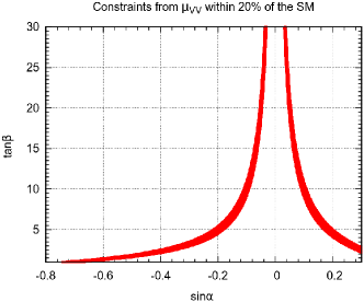
Figure 1: Constraints from $0.8\leq\mu_{VV}\leq 1.2$ on the $\sin{\alpha}$-$\tan{\beta}$ plane.

The left branch corresponds to the right-sign and lies very close to the line $\sin{(\beta-\alpha)}=1$ ($k_{D}=1$), while the right branch corresponds to the wrong-sign and lies very close to the line $\sin{(\beta+\alpha)}=1$ ($k_{D}=-1$).

We note that, because both factors in Eq. (13) get closer to one in the right-sign and wrong-sign limits, a moderate precision in $\mu_{VV}$ implies a very precise line in the $\sin{\alpha}$-$\tan{\beta}$ plane Fontes:2014tga . As shown in detail in section IIB of Fontes:2014tga , for $\tan{\beta}=10$ and a precision of $20\%$ in $\mu_{VV}$, $\sin^{2}{(\beta-\alpha)}$ is determined to better than $0.5\%$ in the wrong-sign branch.

III The $h\rightarrow\Upsilon\gamma$ decay in 2HDM

III.1 Decay rate

The $h\rightarrow\Upsilon\gamma$ decay rate may be written as

$$\Gamma[h\rightarrow\Upsilon\gamma]=\frac{1}{8\pi}\frac{m_{h}^{2}-m_{\Upsilon}^{2}}{m_{h}^{2}}\left|{\cal A}_{\textrm{direct}}+{\cal A}_{\textrm{indirect}}\right|^{2}.$$ (17)

The direct diagram is shown in Fig. 2(b) and arises from the direct $hb\bar{b}$ coupling ($k_{D}$). The indirect diagram is shown in Fig. 2(a) and arises from the effective $h\gamma\gamma$ with a virtual photon morphing into an $\Upsilon$.

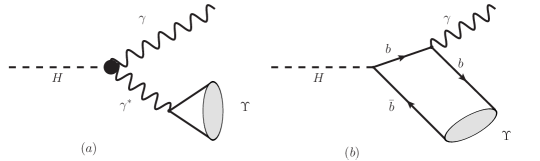
Figure 2: Feynman diagrams contributing to the $h\to\Upsilon\gamma$ process. The diagrams originate from two different couplings: (a) loop induced $h\gamma\gamma$ (indirect) coupling; (b) $hb\bar{b}$ Yukawa (direct) coupling.

We adapt the calculations of Ref. Bodwin:2013gca to the 2HDM, and write

$${\cal A}_{\textrm{direct}} = -\eta\,\frac{2}{\sqrt{3}}e\,k_{D}\left(\sqrt{2}G_{F}\frac{m_{\Upsilon}}{m_{h}}\right)^{1/2}\frac{m_{h}^{2}-m_{\Upsilon}^{2}}{m_{h}^{2}-m_{\Upsilon}^{2}/2-2m_{b}^{2}}\ \phi_{0}(\Upsilon),$$

$${\cal A}_{\textrm{indirect}} = \frac{e\,g_{\Upsilon\gamma}}{m_{\Upsilon}^{2}}\left(\sqrt{2}G_{F}\right)^{1/2}\frac{\alpha}{\pi}\frac{m_{h}^{2}-m_{\Upsilon}^{2}}{\sqrt{m_{h}}}\frac{X}{4},$$ (18)

where $G_{F}$ is Fermi’s constant, $e$ is the positron charge, $k_{D}$ is given in Eq. (10), $m_{\Upsilon}$ and $m_{b}$ are the $\Upsilon$ and b-quark masses, $\alpha$ is the fine-structure constant, $\phi_{0}^{2}(\Upsilon)\sim 0.512$ $\textrm{GeV}^{3}$ is the wave function of $\Upsilon$ at the origin, and

$$g_{\Upsilon\gamma}=\frac{2}{\sqrt{3}}\sqrt{m_{\Upsilon}}\,\phi_{0}(\Upsilon),$$ (19)

whose magnitude can be determined from

$$\Gamma[\Upsilon\rightarrow\ell^{+}\ell^{-}]=\frac{4\pi\alpha^{2}(m_{\Upsilon})}{3m_{\Upsilon}^{3}}g_{\Upsilon\gamma}^{2}.$$ (20)

Our expressions in Eqs. (18) bear three differences with respect to Eqs. (14a)-(14b) of Ref. Bodwin:2013gca . First, we have included explicitly in ${\cal A}_{\textrm{direct}}$ the factor $\eta=0.689$ mentioned at the end of section IIA of Bodwin:2013gca , due to the full NLO corrections Bodwin:2013gca ; Bodwin:2014bpa . Second, we have corrected in ${\cal A}_{\textrm{indirect}}$ a $\sqrt{2}$ misprint. Finally, we have defined ${\cal I}=-X/4$, where $X$ is the function arising from the calculation of the effective $h\gamma\gamma$ coupling at one-loop in the 2HDM, which can be found in appendix B of Ref. Fontes:2014xva .

As shown in Bodwin:2013gca , the direct and indirect contributions interfere destructively in an almost complete manner in the SM, and $h\rightarrow\Upsilon\gamma$ cannot be detected. This is also the case in the right-sign solution of the 2HDM. In contrast, the wrong-sign solution has a constructive interference, raising the prospects for detection. This is what we turn to next.

III.2 The importance of $h\rightarrow\Upsilon\gamma$ for the wrong-sign scenario

As mentioned, the experimental measurement of $\mu_{VV}$ means that the $hVV$ and $ht\bar{t}$ couplings lie close to their SM values. As a result, $h\rightarrow\gamma\gamma$ in the 2HDM is still dominated by the $W$ loop, with a small destructive interference correction from the top loop. There are two novelties in the 2HDM. First, the alteration of $k_{D}$. The bottom loop contribution is negligible in the SM. It can indeed change sign in the 2HDM, but, since $\mu_{VV}$ places $|k_{D}|\sim 1$, it cannot have a strong impact. Second, there is a charged Higgs loop. This decouples with the mass of the charged Higgs, but it can still give a contribution of up to ten percent for values of the charged Higgs mass around 600 GeV. Such effects are inevitable in the wrong-sign scenario Ferreira:2014naa . One concludes that only precise measurements of the $h\rightarrow\gamma\gamma$ decays can yield a signal for the wrong-sign solution of the 2HDM Ferreira:2014naa ; Fontes:2014tga ; the only method presented thus far.

Here we advocate that $h\rightarrow\Upsilon\gamma$ is a good candidate to determine the sign of $k_{D}$. This occurs precisely because the cancellation is almost complete in the SM. A change in the sign of $k_{D}$ means that the interference becomes constructive, thus increasing by orders of magnitude the $h\rightarrow\Upsilon\gamma$ decay rate. This can be used to constrain the wrong-sign solution in the 2HDM.

We have performed a full simulation of the real 2HDM, including theoretical constraints from bounded from below potential Deshpande:1977rw , perturbative unitarity Kanemura:1993hm ; Akeroyd:2000wc ; Ginzburg:2003fe , oblique radiative parameters Peskin:1991sw ; Grimus:2008nb ; Baak:2012kk , and we keep $m_{H^{\pm}}>480\textrm{GeV}$ to respect B-physics constraints. We include all production mechanisms Spira:1995mt ; Harlander:2012pb ; vbf and take $\mu_{VV}$, $\mu_{\gamma\gamma}$, and $\mu_{\tau\tau}$ to lie within 20% of the SM, in close accordance with the latest LHC constraints Khachatryan:2016vau .

The results of our simulation in the type II model are shown in Fig. 3.

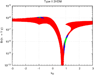
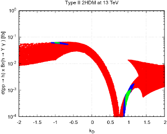
Figure 3: Figure (a): BR($h\rightarrow\Upsilon\gamma$) as a function of $k_{D}$. The red/dark-grey points pass all theoretical constraints in the type II 2HDM. The blue/black (green/light-grey) points pass both the theoretical constraints and the experimental constraints on $\mu_{VV}$, $\mu_{\gamma\gamma}$, and $\mu_{\tau\tau}$ at 20% (10%). Figure (b): Same plot, but for $\sigma(pp\rightarrow h)\times\textrm{BR}(h\rightarrow\Upsilon\gamma)$ at 13 TeV.

The red/dark-grey points pass all theoretical constraints. The blue/black (green/light-grey) points pass those and also $\mu_{VV}$, $\mu_{\gamma\gamma}$, and $\mu_{\tau\tau}$ at 20% (10%). The situation for the flipped model is very similar, with only very slight differences in the allowed regions, due to the different dependence on $\mu_{\tau\tau}$.

There are several features of note. After theoretical constraints, the simulation allows for a very large range of $k_{D}$. Contrary to what one might naively expect, having a large $k_{D}$ does not improve much the $h\rightarrow\Upsilon\gamma$ branching ratio. The point is that, although a large $k_{D}$ does indeed increase the direct amplitude, in accordance with Eq. (18), in the 2HDM the width of $h$ is dominated by $h\rightarrow b\bar{b}$, which also increases with $k_{D}$. Once one introduces the experimental constraints, the values for $k_{D}$ get restricted to right-sign ($k_{D}\sim 1$) and wrong-sign ($k_{D}\sim-1$) regions. As explained in Sec. II.2, this is mostly due to $\mu_{VV}$ and simple trigonometry Fontes:2014tga . Finally, one sees that, due to the same destructive interference at play in the SM, the right-sign solution leads to a minute $h\rightarrow\Upsilon\gamma$ branching ratio around $10^{-8}$. In contrast, the wrong-sign solution leads to constructive interference and a $h\rightarrow\Upsilon\gamma$ branching ratio larger by two orders of magnitude.

The possible experimental reach is best seen in Fig. 3(b), where we show a simulation of $\sigma(pp\rightarrow h)\times\textrm{BR}(h\rightarrow\Upsilon\gamma)$ at 13 TeV. For the wrong-sign, we find a value around $0.06$ fb. The current run II data lies around 15 fb^-1 total integrated luminosity lumi and will ultimately achieve around 100 fb^-1, meaning that a measurement is becoming possible. This $0.06$ fb estimate arises from the precise values taken for $g_{\Upsilon}$ and the scale chosen for $\alpha$ in the various steps of the calculation. A detailed discussion, including relativistic corrections, can be found in Bodwin:2014bpa . Our result presents a lower limit on the number of events, meaning that detection prospects are likely to be superior. Of course, an even better determination is possible at the High-Luminosity LHC, allowing for the detection or completely ruling out of the wrong-sign solution. We have made a simulation at 14 TeV and obtain the expected increase of about $15\%$ from $0.06$ fb into around $0.07$ fb, in both Type II and Flipped.

IV Conclusions

The decay $h\rightarrow\Upsilon\gamma$ is very small in the SM, due to a cancellation between the direct and indirect diagrams. In contrast, in theories with a negative $hbb$ coupling, the interference becomes constructive and the rate is increased by orders of magnitude. We have studied this effect on the wrong-sign solution of the Type II and flipped 2HDM. We make detailed predictions for the number of events consistent with current bounds on the 2HDM and prove that searches for $h\rightarrow\Upsilon\gamma$ constitute a viable and clean method to constrain the wrong-sign solution, especially at a high luminosity facility.