Determining stationary-state quantum properties directly from system-environment interactions

Abstract

Considering stationary states of continuous-variable systems undergoing an open dynamics, we unveil the connection between properties and symmetries of the latter and the dynamical parameters. In particular, we explore the relation between the Lyapunov equation for dynamical systems and the steady-state solutions of a time-independent Lindblad master equation for bosonic modes. Exploiting bona-fide relations that characterize some genuine quantum properties (entanglement, classicality, and steerability), we obtain conditions on the dynamical parameters for which the system is driven to a steady-state possessing such properties. We also develop a method to capture the symmetries of a steady-state based on symmetries of the Lyapunov equation. All the results and examples can be useful for steady-state engineering processes.

The manipulation of the environment affecting the dynamics of a quantum system, with the aim of driving the latter towards a specific state, embodies a valuable tool for quantum state engineering. Depending on assumptions about the couplings, the open dynamics can lead to either an equilibrium state or to a dynamical steady-state. On the other hand, in this scenario, it is critical to ensure that the desired state is achieved regardless the fluctuations in the initial state of the system. Protocols of this sort are known as reservoir engineering, stabilization, and design poyatos ; wiseman ; ticozzi ; albert .

A standard approach to the modeling of the evolution of an open system is the Lindblad master equation (LME) for the density operator $\hat{\rho}$ wiseman ; lindblad ; breuer :

$$\frac{d\hat{\rho}}{dt}=-\frac{i}{\hbar}[\hat{H},\hat{\rho}]-\frac{1}{2\hbar}\!\sum_{m=1}^{M}(\{\hat{L}_{m}^{\dagger}\hat{L}_{m},\hat{\rho}\}-2\hat{L}_{m}\hat{\rho}\hat{L}_{m}^{\dagger}),$$ (1)

which, besides the unitary dynamics ruled by the Hamiltonian operator $\hat{H}$, accounts for a nonunitary dynamics as resulting from the weak coupling (via the operators $\hat{L}_{k}$) to uncontrollable environmental degrees of freedom. The LME is the most general type of Markovian and time-homogeneous master equation guaranteeing trace preservation and complete positivity. Despite the fundamental and very restrictive Markovianity assumption, the LME is crucial for the description of an ample set of dynamics in quantum optics and information, mesoscopic physics, and quantum chemistry wiseman ; albert2 ; breuer .

In this work we investigate properties and symmetries of continuous-variable states driven to equilibrium by a linear evolution governed by the time-independent Lindblad dynamics. Gaussian states, which play a preponderant role in quantum information science and are the natural candidates for the implementation of quantum computation with continuous variables lloyd , belong to such set of states.

From the mathematical point of view, the problem of whether a linear LME has a stable steady-state is equivalent to the solution of a Lyapunov equation for the covariance matrix of the quantum state. The methodology used to solve Lyapunov equations, known as Lyapunov stability theory dullerud , was developed in Ref. lyapunov in the context of dynamical systems. This formalism was explored in Ref. koga to determine conditions for a state to be pure in the stationary regime.

In our work, we make use of the connection between the LME and the Lyapunov theory to determine several properties of continuous-variables steady-states, such as classicality englert , separability simon2 (or bound entanglement werner ), and steerability wiseman2 . Further, we also explore the steady-state symmetries induced by the dynamical symmetries of the Lyapunov equation. This is particularly interesting, because it is in general hard to characterize the symmetries of the states working directly on the LME (1). This task becomes instead fully manageable when dealing with finite matrices. Our results are applicable to systems with a generic number of degrees of freedom and their analyticity brings in turn robustness for numerical examinations of the mentioned properties.

The remaining of this paper is organized as follows: In Sec.I, we set the notation and describe the linear dynamics, discussing the connection between the LME and the Lyapunov theory. The mathematical results concerning the Lyapunov equation are developed in Sec.II, which will be extensively applied to find general properties of stationary solutions in Sec.III. Symmetries of the system are analyzed in Sec.IV, while examples are given in Sec.V. A method for engineering steady-states is presented in Sec.VI. Section VII presents our conclusions, while in the Appendixes we further discuss some technical aspects of the mathematical approach, including a brief summary of the notation.

I Linear Dynamics and Stationary Conditions

For a system of $n$ continuous degrees of freedom (DF), the generalized coordinates together with the canonical conjugated momenta are collected in a $2n$ column vector:

$$\hat{x}:=(\hat{q}_{1},...,\hat{q}_{n},\hat{p}_{1},...\hat{p}_{n})^{\dagger}.$$ (2)

In this notation, the canonical commutation relation (CCR) is written compactly as $[\hat{x}_{j},\hat{x}_{k}]=i\hbar\,\mathsf{J}_{jk}$ with ${\sf J}_{jk}$ given by the elements of the symplectic matrix

$$\mathsf{J}:=\left(\begin{array}[]{cc}{\bf 0}_{n}&\mathsf{I}_{n}\\ -\mathsf{I}_{n}&{\bf 0}_{n}\end{array}\right).$$ (3)

We consider the evolution of a quantum state governed by the LME with a quadratic Hamiltonian and linear Lindblad operators, viz.,

$$\hat{H}=\frac{1}{2}\hat{x}\cdot\mathbf{H}\hat{x}+\xi\cdot\mathsf{J}\hat{x}+H_{0},$$ (4)

$$\hat{L}_{m}=\lambda_{m}\cdot\mathsf{J}\hat{x}+\mu_{m},$$

where $\xi\in\mathbb{R}^{2n}$ and $\lambda_{m}\in\mathbb{C}^{2n}$ are column vectors; $H_{0}\in\mathbb{R}$ and $\mu_{m}\in\mathbb{C}$ are constants and $m=1,...,M$. The Hessian of the Hamiltonian is symmetric by definition: $\mathbf{H}=\mathbf{H}^{\top}\in{\rm Mat}(2n,\mathbb{R})$. Under such conditions, the evolution of the mean value vector $\langle\hat{x}\rangle_{t}:={\rm Tr}\left[\hat{x}\hat{\rho}(t)\right]\in\mathbb{R}^{2n}$ can be retrieved from (1) by using only the CCR nicacio ; wiseman :

$$\frac{d\langle\hat{x}\rangle_{t}}{dt}=\xi-\eta+{\bf\Gamma}\langle\hat{x}\rangle_{t},$$ (5)

where we have introduced $\eta:=\sum_{m=1}^{M}{\rm Im}(\mu_{m}^{\ast}\,\lambda_{m})\in{\mathbb{C}}^{2n}$,

$${\bf\Gamma}:=\mathsf{J}\mathbf{H}-{\rm Im}{\bf\Upsilon}\mathsf{J}\in{\rm Mat}(2n,\mathbb{R}),$$ (6)

and

$${\bm{\Upsilon}}:=\sum_{m=1}^{M}\lambda_{m}\lambda_{m}^{\dagger}\in{\rm Mat}(2n,\mathbb{C}).$$ (7)

The natural question that arises at this point is whether a solution of (5) attains a finite asymptotic value when $t\to\infty$. The answer is provided in the context of the Lyapunov stability theory dullerud . All solutions will be driven to an asymptotic point, if the matrix $\bf\Gamma$ is asymptotically stable (AS), i.e., if its spectrum has negative real part.

Interestingly enough, from the Lindblad dynamics (1) with the operators in Eq.(4), a Lyapunov equation (LE) emerges naturally for the stationary value of the covariance matrix (CM) of the system, as we shall see. Defining the CM of the state $\hat{\rho}$ as ${\bf V}={\bf V}^{\top}\in{\rm Mat}(2n,\mathbb{R})$ with elements note1

$$\mathbf{V}_{\!jk}=\tfrac{1}{\hbar}{\rm Tr}\left[\left\{\hat{x}_{j}-\langle\hat{x}_{j}\rangle_{t},\hat{x}_{k}-\langle\hat{x}_{k}\rangle_{t}\right\}\hat{\rho}(t)\right],$$ (8)

and calculating its evolution nicacio ; wiseman , the (possible) stationary value of the CM will be the solution of the LE

$${\bf V}{\bf\Gamma}^{\!\top}+{\bf\Gamma}{\bf V}+{\bf D}=0,$$ (9)

with $\bf\Gamma$ in (6) and

$${\bf D}:=2\,{\rm Re}{\bf\Upsilon}={\bf D}^{\!\top}\in{\rm Mat}(2n,\mathbb{R}),$$ (10)

which is positive semidefinite, ${\bf D}\geq 0$, by the definition of $\bf\Upsilon$. The Lyapunov theorem and its extensions lyapunov ; horn ; dullerud guarantee that for an AS matrix $\bf\Gamma$, the solution of Eq.(9) exists and is unique. Furthermore, those theorems also relate the stability nature of the matrix $\bf\Gamma$ to the existence of matrices (in our case $\bf V$ and $\bf D$) satisfying the LE (9).

We stress that, in order to deduce Eqs.(5) and (9), we do not need any assumptions about the initial state of the system. The derivation of such equations only uses the LME, the particular structure of Eqs. (4), and the CCR. Meanwhile, the LME with the operators (4) will always preserve the Gaussian character of an initial Gaussian state nicacio . Once the CM of a steady-state of the system is a solution of (9), which is unique and does not depend on the initial state, any initial state will end in a Gaussian steady-state.

II Lyapunov Equations

In this section we show and develop results concerning the generic Lyapunov equation

$${\bf A}\,{\bf P}+{\bf P}{\bf A}^{\!\dagger}+{\bf Q}=0,$$ (11)

and its solution. Since our objective is to understand properties of stationary solutions of the LME, it is convenient to assume that (i) ${\bf A}\in{\rm Mat}(m,\mathbb{C})$ is AS, (ii) ${\bf P}={\bf P}^{\dagger}\in{\rm Mat}(m,\mathbb{C})$ and (iii) ${\bf Q}={\bf Q}^{\dagger}\in{\rm Mat}(m,\mathbb{C})$. From now on, the LE (11) will be represented by the triple $\lfloor{\bf P},{\bf A},{\bf Q}\rceil$.

The first of those assumptions (${\bf A}$ is AS) is enough to prove horn ; dullerud that the unique solution for the LE in (11) is written as

$${\bf P}({\bf Q},{\bf A})=\int_{0}^{\infty}\!\!\,dt\,\,{\rm e}^{{\bf A}t}\,{\bf Q}\,\,{\rm e}^{{\bf A}^{\!\dagger}t}\,.$$ (12)

Furthermore, for any ${\bf A}\in{\rm GL}(m,\mathbb{C})$, it is true that

$${\rm In}\left({\rm e}^{{\bf A}t}\,{\bf Q}\,\,{\rm e}^{{\bf A}^{\!\dagger}t}\right)={\rm In}\left({\bf Q}\right),$$ (13)

because the expression inside the parenthesis on the LHS is a congruence transformation of $\bf Q$. The symbol “$\rm In$” refers to the inertia index of a matrix, as defined in Appendix I. On the other hand, once ${\bf A}$ is AS, then $\lim_{t\to\infty}{\rm e}^{{\bf A}t}=0$, which guarantees the convergence of the integral in (12). These last arguments about the structure of Eq.(12) are used in the proof of the following result dullerud ; horn :

Proposition 1.

Consider the solution (12) for the LE in (11). If ${\bf Q}\geq 0$ (resp. ${\bf Q}>0$), then ${\bf P}\geq 0$ (resp. ${\bf P}>0$) .

Note that Prop.1 does not exclude the statement ${\bf Q}\geq 0\Longrightarrow{\bf P}>0$, since the set of matrices ${\bf P}$ such that ${\bf P}>0$ is a subset of ${\bf P}\geq 0$, cf. Appendix I. This is the case provided the pair $({\bf Q},{\bf A})$ is observable horn ; dullerud . For our purposes, this statement is not necessary, however it is for the results in koga .

Now, let us go a bit further with the results in Prop.1, specializing the properties of the AS matrix $\bf A$:

Proposition 2.

Consider the LE $\lfloor{\bf P},{\bf A},{\bf Q}\rceil$ with ${\bf A}={\bf A}^{\!\dagger}$, then ${\bf P}\geq 0$ (resp. ${\bf P}>0$) if and only if ${\bf Q}\geq 0$ (resp. ${\bf Q}>0$).

Proof.

Since ${\bf A}$ is self-adjoint and negative definite ( AS), it is possible to write ${\bf A}=-\sqrt{-{\bf A}}\sqrt{-{\bf A}}$, where $\sqrt{-{\bf A}}$ is the unique self-adjoint positive definite square root of $-{\bf A}$. From the LE (11),

$$\!\!\!\!\!{\rm Spec}_{\mathbb{R}}({\bf Q}) = -{\rm Spec}_{\mathbb{R}}\left({\bf A}{\bf P}+{\bf P}{\bf A}\right)$$

$$= -{\rm Spec}_{\mathbb{R}}\left[\left({\bf P}+{\bf A}{\bf P}{\bf A}^{-1}\right){\bf A}\right]$$

$$= {\rm Spec}_{\mathbb{R}}\left[\sqrt{-{\bf A}}\left({\bf P}+{\bf A}{\bf P}{\bf A}^{-1}\right)\sqrt{-{\bf A}}\right]\!.$$

Since the sum of positive semidefinite (resp. positive definite) matrices is positive semidefinite (resp. positive definite), and since a congruence transformation does not change the signs of the eigenvalues [or the inertia of the matrix], it follows that ${\bf Q}\geq 0$ (resp. ${\bf Q}>0$) if ${\bf P}\geq 0$ (resp. ${\bf P}>0$), which proves the necessary condition. The sufficiency is in Prop.1. ∎

Note that, once one statement in Prop.2 is ${\bf Q}>0\Longleftrightarrow{\bf P}>0$, then the statement ${\bf Q}\geq 0\Longleftrightarrow{\bf P}\geq 0$ necessarily means that if $\bf Q$ has one null eigenvalue, then $\bf P$ will also have, and vice-versa.

In the direction of the main task of this work, we must develop some results concerning matrices of the form ${\bf P}+{\bf\Xi}$, where ${\bf P}$ is the solution in Eq.(12) of $\lfloor{\bf P},{\bf A},{\bf Q}\rceil$ and ${\bf\Xi}={\bf\Xi}^{\dagger}\in{\rm Mat}(m,\mathbb{C})$.

Corollary 1.

${\bf P}+{\bf\Xi}\geq 0$   if   ${\bf Q}_{[\bf\Xi]}:={\bf Q}-{\bf\Xi A}^{\dagger}-{\bf A\Xi}\geq 0$.

Proof.

It is easy to see that the LE $\lfloor{\bf P}+{\bf\Xi},{\bf A},{\bf Q}_{[\bf\Xi]}\rceil$ is equivalent to the LE in (11). Thus, the proof follows from Prop.1, since ${\bf Q}_{[\bf\Xi]}={\bf Q}_{[\bf\Xi]}^{\dagger}$. ∎

The converse statement of Corol.1 is not true in general. By using the restriction for the matrices $\bf A$, as in Prop.2, we obtain the following corollary giving a necessary and sufficient condition.

Corollary 2.

Consider ${\bf A}={\bf A}^{\!\dagger}$ ($\bf A$ is AS), then ${\bf P}+{\bf\Xi}\geq 0$   if and only if   $\widetilde{\bf Q}_{[{\bf\Xi}]}:={\bf Q}-{\boldsymbol{\{}}{\bf\Xi,A}{\boldsymbol{\}}}_{\!+}\geq 0$.

Proof.

As before, we construct the equivalent Lyapunov equation $\lfloor{\bf P}+{\bf\Xi},{\bf A},\widetilde{\bf Q}_{[\bf\Xi]}\rceil$, and use Prop.2 since $\widetilde{\bf Q}_{[\bf\Xi]}\!=\!\widetilde{\bf Q}_{[\bf\Xi]}^{\dagger}$. ∎

Note that, contrary to Props. 1 and 2, we did not mention the strictly positive cases (${\bf Q}_{[\bf\Xi]}\!>\!0$, $\widetilde{\bf Q}_{[\bf\Xi]}\!>\!0$) in Corols. 1 and 2. Actually, these cases follow the same prescription, but they are not necessary for our next results.

In what follows, properties of the steady states, driven to equilibrium under the linear evolution generated by (4), will be considered from the perspective of the results developed in this section.

III Bona-Fide Relations and Steady-States

Through the temporal evolution of a state by the LME conditioned to an AS dynamics, the dependence on the initial condition is progressively erased by the environmental action. Therefore the steady-state properties must be completely determined only by the environment. An usual way to describe properties of continuous-variable states is given by bona-fide relations involving the CM of the states. From now on, we will assume that the CM of a quantum state evolves with $\bf\Gamma$ AS and ${\bf D}\geq 0$ and attains an asymptotic value described by the LE (9) with solution ${\bf V}:={\bf P}({\bf D},{\bf\Gamma})$ in Eq.(12).

It is convenient to recall the definitions of the auxiliary matrices defined in Corols. 1 and 2, but now for the LE in question. For any matrix ${\bf\Xi}={\bf\Xi}^{\dagger}\in{\rm Mat}(2n,\mathbb{C})$, we have

$${\bf D}_{[\bf\Xi]}:={\bf D}-{\bf\Xi\,\Gamma}{\!{}^{\top}}-{\bf\Gamma\,\Xi},\,\,\,\widetilde{\bf D}_{[{\bf\Xi}]}:={\bf D}-{\boldsymbol{\{}}{\bf\Xi,\Gamma}{\boldsymbol{\}}}_{\!+}.$$ (15)

III.1 Uncertainty Principle

Any quantum state is subjected to constrains imposed by the uncertainty principle, which is only a consequences of the CCR. For the continuous-variables case, this principle takes into account only the CM (8). A genuine physical state has a CM such that simon

$${\bf V}+i\mathsf{J}_{2n}\geq 0.$$ (16)

Given a Hamiltonian and a collection of Lindblad operators as in (4), what can our corollaries say about the genuineness of the steady-state generated by the LME? Invoking Corol.1, the matrix $\bf V$ of a steady-state is a bona-fide CM if ${\bf D}_{[i\mathsf{J}]}={\bf D}-i{\bf\Gamma}\mathsf{J}-i\mathsf{J}{\bf\Gamma}^{\!\top}\geq 0$. However, using Eqs. (6) and (7), it is not difficult to show that ${\bf D}_{[i\mathsf{J}]}=2{\bf\Upsilon}^{\ast}$, which is always positive semidefinite, according to the definition of ${\bf\Upsilon}$ in (7). Tautologically, this says that all linear LMEs with $\bf\Gamma$ AS and ${\bf D}\geq 0$ will drive the system to a steady-state obeying the relation (16), i.e., a genuine physical state.

On the other hand, Eq.(9) is a consequence of the CCR, as mentioned before. Accordingly, the LME guarantees that the uncertainty principle holds for all times, including the steady-state limit, whereof the condition in Corol.1 is necessary and sufficient regardless of whether $\bf\Gamma$ is symmetric. Before going to the next bona-fide relation, it is important to remark that this extension of Corol.1 to an “if and only if” condition is only true for the relation in Eq.(16). For all the other relations which will appear in what follows, the differences between Corols. 1 and 2 should be considered.

III.2 Classical States

Classical States are defined as having a positive Glauber-Sudarshan distribution function, they are also called P-representable states. This definition relies on the possibility to express a desired state as a classical mixture of coherent states. The necessary and sufficient condition for P-representability of a Gaussian state is written in terms of its CM as the bona-fide relation (see Appendix II)

$${\bf V}-\mathsf{I}_{2n}\geq 0.$$ (17)

The evolution that drives the system to a classical steady-state is subjected to the sufficient condition given by Corol.1:

$${\bf D}_{[-\mathsf{I}]}={\bf\Gamma}+{\bf\Gamma}^{\!\top}+{\bf D}\geq 0\Longrightarrow{\bf V}-\mathsf{I}_{2n}\geq 0.$$ (18)

The contrapositive of the above statement says that if a given LME is such that ${\bf D}_{[-\mathsf{I}]}$ has at least one negative eigenvalue, it will lead the system to a nonclassical stationary state. The matrix ${\bf V}$ is, by hypothesis, the CM of a steady-state of the LME. Once the converse statement of (18) is not true, one can conclude that there are classical steady-states which can not be generated by a LME with dynamical matrices such that ${\bf D}_{[-\mathsf{I}]}\geq 0$.

If we consider only steady-states generated by a LME with ${\bf\Gamma}$ symmetric, by Corol.2 the possible classical states will obey the necessary and sufficient condition

$$\widetilde{\bf D}_{[-\mathsf{I}]}=2{\bf\Gamma}+{\bf D}\geq 0\Longleftrightarrow{\bf V}-\mathsf{I}_{2n}\geq 0.$$ (19)

This means that all states generated by a LME with ${\bf\Gamma}={\bf\Gamma}^{\!\top}$ and $\widetilde{\bf D}_{[-\mathsf{I}]}\geq 0$ are classical states. Conversely, all classical states with CM $\bf V$ which are solutions of a LE with ${\bf\Gamma}={\bf\Gamma}^{\!\top}$ are steady-states of a LME satisfying $\widetilde{\bf D}_{[-\mathsf{I}]}\geq 0$.

Since classicality is related to mixtures of coherent states, one instructive example is given by the CM ${\bf V}=\mathsf{I}_{2n}$ — i.e., the CM of any $n$-mode (or $n$- DF) coherent state. The simplicity of this case enables us to derive an useful necessary and sufficient condition besides the relation in Eq.(19). Actually, we will be concerned with the slightly more general situation: the tensor product of $n$ Gibbs-states with the same occupation number. These states have the global CM written as ${\bf V}=\alpha\mathsf{I}_{2n}$, which is a CM of a classical state if $\alpha\geq 1$.

Corollary 3.

For any $\alpha>0$ and any $\bf\Gamma$ such that $({\bf\Gamma}+{\bf\Gamma}^{\!\top})\leq 0$, the matrix ${\bf V}=\alpha\,\mathsf{I}_{2n}$ is a solution of the LE $\lfloor{\bf V},{\bf\Gamma},{\bf D}\rceil$ if and only if $\alpha({\bf\Gamma}+{\bf\Gamma}^{\!\top})+{\bf D}=0$. Furthermore, $\alpha=\tfrac{1}{2}{\rm Tr}{\bf D}/{\rm Tr}({\rm Im}{\bf\Upsilon}\mathsf{J})$.

Proof.

The sufficient condition is trivially obtained by constructing the LE $\lfloor\alpha\mathsf{I}_{2n},{\bf\Gamma},{\bf D}\rceil$ from (9). To prove the necessary condition, one defines

$$\mathcal{I}:=\int^{\infty}_{0}\!\!\!dt\,{\rm e}^{{\bf\Gamma}t}\,{\rm e}^{{\bf\Gamma}^{\!\top}\!t}$$

and integrates it by parts to show that $\mathcal{I}\,{\bf\Gamma}^{\!\top}\!+\!{\bf\Gamma}\,\mathcal{I}=-\mathsf{I}_{2n}$. The solution (12) with ${\bf Q}={\bf D}=-\alpha({\bf\Gamma}+{\bf\Gamma}^{\!\top})$ and ${\bf A}={\bf\Gamma}$ shows that ${\bf V}=-\alpha({\bf\Gamma}\,\mathcal{I}+\mathcal{I}\,{\bf\Gamma}^{\!\top})=\alpha\mathsf{I}$. Since ${\bf\Gamma}\in{\rm Mat}(2n,\mathbb{R})$, its complex eigenvalues will occur in conjugate pairs, then ${\rm Tr}\,{\bf\Gamma}\in\mathbb{R}$. Since it is also AS, ${\rm Tr}\,{\bf\Gamma}\neq 0$, then the value of $\alpha$ holds if one considers the definition of $\bf\Gamma$ in Eq.(6) and the fact that ${\rm Tr}(\mathsf{J}{\bf H})=0$, since $\bf H$ is symmetric. ∎

The state studied in Corol.3 is an example of the multiplicity of the steady-state with respect to different matrices $\bf\Gamma$ and $\bf D$. There is an infinite number of matrices satisfying the relation $\alpha({\bf\Gamma}+{\bf\Gamma}^{\!\top})+{\bf D}=0$ and giving rise to the same steady state. However, for a given pair of matrices $\bf\Gamma$ and $\bf D$, the solution ${\bf V(\Gamma,D)}$ is uniquely given in Eq.(12).

III.3 Separable States

A necessary and sufficient condition for an $n$-mode Gaussian state to be separable with respect to one of the modes, say the $k^{\underline{\text{th}}}$ one, is defined in terms of its CM as ${\bf V}^{\!\top_{\!\!k}}+i\mathsf{J}\geq 0$, where ${\bf V}^{\!\top_{\!\!k}}:={\bf T}_{\!k}{\bf V}{\bf T}_{\!k}$. The transformation ${\bf T}_{\!k}={\bf T}_{\!k}^{-1}={\bf T}_{\!k}^{\top}$ is a local time inversion on the $\hat{x}$ operator, viz.,

$${\bf T}_{\!k}\hat{x}=(\hat{q}_{1},...,\hat{q}_{k},...,q_{n},\hat{p}_{1},...,-\hat{p}_{k},...,\hat{p}_{n})^{\top}$$ (20)

and, of course, can not be implemented unitarily. Since ${\bf T}_{\!k}$ is orthogonal, we can express the separability condition equivalently as simon2 ; werner

$${\bf V}+i\mathsf{J}^{\!\top_{\!\!k}}\geq 0.$$ (21)

The statements in Eqs. (18) and (19) can be readily modified to the present case:

$$(\text{Corollary\leavevmode\nobreak\ \ref{cor:if}})\,\,\,{\bf D}_{[i\mathsf{J}^{\!\top_{\!\!k}}]}\geq 0 \Longrightarrow {\bf V}+i\mathsf{J}^{\!\top_{\!\!k}}\geq 0;$$ (22a)

$$(\text{Corollary\leavevmode\nobreak\ \ref{cor:iff}})\,\,\,\widetilde{\bf D}_{[i\mathsf{J}^{\!\top_{\!\!k}}]}\geq 0 \Longleftrightarrow {\bf V}+i\mathsf{J}^{\!\top_{\!\!k}}\geq 0.$$ (22b)

The interpretations of these conditions are also readily adapted from those in the previous subsection, it is just a question of changing the dichotomy “classical/nonclassical” to “separable/entangled”.

All classical states (not only the Gaussian ones) are separable, since they are written as a convex sum of coherent states which are separable [see Eq.(A-1)]. As a consequence, a hierarchy of the dynamics of LMEs can be established: the set of matrices such that $\widetilde{\bf D}_{[-\mathsf{I}]}\geq 0$ in (19) is a subset of those satisfying $\widetilde{\bf D}_{[i\mathsf{J}^{\!\top_{\!\!k}}]}\geq 0$ in (22b). However, this is not true for the matrices in (18) and (22a), because both only give a sufficient condition.

Now, consider the following partition of the number of DF of a state: $n=n_{1}+n_{2}$, where $n_{i}$ is the number of DF of each partition. Define also the local time inversion operation as

$$\!\!{\bf T}_{\!n_{2}}\hat{x}=\!(\hat{q}_{1},...,\hat{q}_{n},\hat{p}_{1},...,\hat{p}_{n_{1}},-\hat{p}_{n_{1}+1},...,-\hat{p}_{n_{1}+n_{2}})^{\top}\!.$$ (23)

The separability criteria already exposed is a necessary and sufficient condition only if $n_{2}=1$. For all other cases, entangled states with ${\bf V}+i{\bf T}_{\!n_{2}}\mathsf{J}{\bf T}_{\!n_{2}}\geq 0$ are bound entangled, i.e., they have nondistillable entanglement werner . One can also relate the reservoir properties with this bona-fide relation through the replacement $\mathsf{J}^{\!\top_{\!\!k}}\to{\bf T}_{\!n_{2}}\mathsf{J}{\bf T}_{\!n_{2}}$ in Eqs.(22). Note that the bona-fide relation in question does not say whether the state is separable or bound-entangled.

III.4 Gaussian Steerability

Quantum Steering is a form of correlation related to the ability of one part of a system to modify the state of a companion system when only local-measurements are performed on the former. More precisely, if through local measurements and classical communication one part of the system is able to convince the other part that they share an entangled state, the state is said to be steerable with respect to the first part wiseman .

As in the previous subsection, considering the partition of the DF as $n=n_{1}+n_{2}$, a state is non-Gaussian-steerable with respect to the first part (with $n_{1}$ DF) if and only if wiseman2

$${\bf V}+i\,{\bf\Pi}_{2}\geq 0,\,\,\,{\bf\Pi}_{2}:=\tfrac{1}{2}(\mathsf{J}+{\bf T}_{\!n_{2}}\mathsf{J}{\bf T}_{\!n_{2}}),$$ (24)

with ${\bf T}_{\!n_{2}}$ defined in (23). In other words, it is not possible to steer the state of part 1, making local Gaussian measurements on part 2, if the last condition holds. The steering relation with respect to the second part is obtained by changing the roles of $n_{1}$ and $n_{2}$.

As before, this concept can be related to the dynamical matrices, and one can derive similar formulas by just replacing $\mathsf{J}^{\!\top_{\!\!k}}\to{\bf\Pi}_{2}$ in (22). All Gaussian steerable states are entangled wiseman , thus the set of matrices such that $\widetilde{\bf D}_{[i{\bf\Pi}_{2}]}\geq 0$ is a subset of the ones satisfying $\widetilde{\bf D}_{[i\mathsf{J}^{\!\top_{\!\!k}}]}\geq 0$.

This concludes our analysis of the bona-fide relations used across this paper.

IV Symmetries of Steady-States

In principle, symmetries of the steady-states can be associated with the symmetries of the dynamics governed by the LME albert ; albert2 . In the perspective developed in this work, the relation of the steady-state symmetries and the symmetries of the dynamical matrices ${\bf\Gamma}$ and ${\bf D}$ will be investigated.

Two LEs, $\lfloor{\bf V},{\bf\Gamma},{\bf D}\rceil$ and $\lfloor{\bf V}^{\prime},{\bf\Gamma}^{\prime},{\bf D}^{\prime}\rceil$, are said to be covariant when their matrices are related by

$${\bf V^{\prime}}=\mathbf{W}{\bf V}\mathbf{W}^{\!\top},\,\,\,{\bf\Gamma^{\prime}}=\mathbf{W}{\bf\Gamma}\mathbf{W}^{-1},\,\,\,{\bf D^{\prime}}=\mathbf{W}{\bf D}\mathbf{W}^{\!\top},$$ (25)

for $\mathbf{W}\in{\rm GL}(2n,\mathbb{R})$. Note that, for an orthogonal $\bf W$, all above matrices are subjected to the same transformation. This covariance is helpful to determine the invariance properties of a steady-state, working directly at the level of the CM:

Proposition 3.

If $\mathbf{\Gamma}$ and ${\bf D}$ are invariant under ${\bf W}\in{\rm GL}(2n,\mathbb{R})$ [i.e., ${\bf W}{\bf\Gamma}{\bf W}^{-1}={\bf\Gamma}$ and ${\bf W}{\bf D}{\bf W}^{\!\top}={\bf D}$], then ${\bf V}$ is invariant as well [i.e., ${\bf W}{\bf V}{\bf W}^{\!\top}={\bf V}$]. In this case, we say that $\mathbf{W}$ is a symmetry transformation of the Lyapunov equation.

Proof.

Writing the solution ${\bf V}({\bf\Gamma},{\bf D})$ as in Eq.(12) for the LE $\lfloor{\bf V},{\bf\Gamma},{\bf D}\rceil$, and since $\det{\bf W}\neq 0$, it is easy to see that ${\bf V}({\bf\Gamma},{\bf D})={\bf V}({\bf W}{\bf\Gamma}{\bf W}^{-1},{\bf W}{\bf D}{\bf W}^{\top})$, i.e., $\bf V$ remains unchanged. ∎

Let us give some particular but useful examples. Consider the transformation

$$\mathbf{W}=\hat{\sigma}_{z}\otimes\mathsf{I}_{2}=\left(\begin{array}[]{cc}\mathsf{I}_{2}&0_{2}\\ 0_{2}&-\mathsf{I}_{2}\end{array}\right)\in{\rm GL}(4,\mathbb{R}).$$ (26)

If $\bf\Gamma$ and $\bf D$ are invariant under this transformation, they are necessarily written as ${\bf\Gamma}={\bf\Gamma}_{1}\oplus{\bf\Gamma}_{2}$ and ${\bf D}={\bf D}_{1}\oplus{\bf D}_{2}$, where ${\bf\Gamma}_{j}$, ${\bf D}_{j}\in{\rm Mat}(2,\mathbb{R})$. As a consequence of Prop.3, ${\bf V}={\bf V}_{1}\oplus{\bf V}_{2}$, i.e., it will be the CM of a state without position-momentum correlations. This invariance can be retrieved directly from the solution (12): if $\bf A$ and $\bf Q$ are block-diagonals then $\bf P$ will also be block diagonal.

Another example is the transformation

$$\mathbf{W}=\left(\begin{array}[]{cc}0_{2}&\mathsf{I}_{2}\\ \mathsf{I}_{2}&0_{2}\end{array}\right)\in{\rm GL}(4,\mathbb{R}).$$ (27)

If $\bf\Gamma$ and $\bf D$ are invariant under this, the CM will have momentum correlations equal to position correlations:

$$\mathbf{V}=\left(\begin{array}[]{cc}{\bf V}_{\!1}&{\bf V}_{12}\\ {\bf V}_{12}&{\bf V}_{\!1}\end{array}\right).$$ (28)

Focusing on the symplectic group, i.e., choosing ${\bf W}\in\mathrm{Sp}(2n,\mathbb{R})\subset{\rm GL}(2n,\mathbb{R})$, we use the definition of $\bf\Gamma$ in (6) and the covariance relation (25) to write

$${\bf V}^{\prime}={\bf W}{\bf V}{\bf W}^{\!\top},\,{\bf H}^{\prime}={\bf W}^{-\top}\!{\bf H}{\bf W}^{-1},\,\lambda^{\prime}={\bf W}{\lambda}.$$ (29)

This symplectic covariance, by the Stone-von Neumann theorem gosson , is nothing but the representation of a unitary transformation of the LME:

$$\hat{\rho}\longrightarrow\hat{\mathrm{U}}{\hat{\rho}}\hat{\mathrm{U}}^{\dagger},\,\,\,{\hat{H}}\longrightarrow\hat{\mathrm{U}}{\hat{H}}\hat{\mathrm{U}}^{\dagger},\,\,\,{\hat{L}_{i}}\longrightarrow\hat{\mathrm{U}}{\hat{L}}_{i}\hat{\mathrm{U}}^{\dagger},$$ (30)

where the unitary operator $\hat{\mathrm{U}}$ is the Metaplectic operator associated with ${\bf W}\in\mathrm{Sp}(2n,\mathbb{R})$ nicacio ; gosson .

If we rearrange the elements of (8) consistently with the reordering $\hat{x}\mapsto\check{x}:=(\hat{q}_{1},\hat{p}_{1},...,\hat{q}_{n},\hat{p}_{n})$ of (2), then the invariance under the (nonreordered) transformation in (26) implies that the steady-state of the system, with CM ${\bf V}={\bf V}_{1}\oplus{\bf V}_{2}$, is the product state $\hat{\rho}=\hat{\rho}_{1}\otimes\hat{\rho}_{2}$. In the reordered basis, the transformation (26) is symplectic. Similarly, the (nonreordered) matrix in (27) is also symplectic in the reordered basis, and it realizes the exchange of the subsystems. Consequently, the matrix in (28) is the CM of states with same local purity (symmetric states).

As a last example, consider a symplectic rotation $\mathsf{R}\in{\rm K}(n):={\rm Sp}(2n,\mathbb{R})\cap{\rm O}(2n)$. As a consequence of its symplecticity and orthogonality, it is written as simon

$$\mathsf{R}=\left(\begin{array}[]{cc}\mathbf{Y}&\mathbf{Z}\\ -\mathbf{Z}&\mathbf{Y}\end{array}\right)$$ (31)

with $\mathbf{Y},\mathbf{Z}\in{\rm Mat}(n,\mathbb{R})$ satisfying the following conditions:

$$\mathbf{Y}\mathbf{Y}^{\!\top}+\mathbf{Z}\mathbf{Z}^{\!\top}=\mathsf{I}_{n},\,\,\,\,\mathbf{Y}\mathbf{Z}^{\!\top}-\mathbf{Z}\mathbf{Y}^{\!\top}=0_{n}.$$ (32)

Any matrix written as ${\bf M}:=m_{1}\mathsf{I}_{2n}+m_{2}\mathsf{J}\in{\rm Mat}(2n,\mathbb{R}),$ with $m_{1},m_{2}\in\mathbb{R}$ is invariant under the whole group ${\rm K}(n)$. Note that, if ${\bf M}={\bf M}^{\!\top}$, then $m_{2}=0$. If we consider

$${\bf\Gamma}=-\gamma_{1}\mathsf{I}_{2n}+\gamma_{2}\mathsf{J},\,\,\,{\bf D}=\delta\mathsf{I}_{2n},$$ (33)

i.e., both invariant under ${\rm K}(n)$, then Prop.3 implies that ${\bf V}=\nu\,\mathsf{I}_{2n}$. By the other side, Corol.3 is a necessary and sufficient condition for this CM, thus $\nu=\tfrac{\gamma}{2\delta}$. It is important to mention that the matrices $\bf\Gamma$ and $\bf D$ on that corollary need not to be invariant.

The subgroup of local rotations in ${\rm K}(n)$ is described as the set of matrices (31) with

$$\mathbf{Y}={\rm Diag}(y_{1},y_{2},...,y_{n}),\,\,\,\mathbf{Z}={\rm Diag}(z_{1},z_{2},...,z_{n}),$$ (34)

which corresponds to a rotation

$${\sf R}_{i}:=\begin{pmatrix}y_{i}&z_{i}\\ -z_{i}&y_{i}\end{pmatrix}\in{\rm K}(1)$$ (35)

in each respective canonical pair $(\hat{q}_{i},\hat{p}_{i})$. The matrix ${\bf\Gamma}\in{\rm Mat}(2n,\mathbb{R})$ is invariant under the local rotation subgroup if it is of the following form:

$${\bf\Gamma}=\begin{pmatrix}{\bf\Gamma}_{1}&{\bf\Gamma}_{2}\\ -{\bf\Gamma}_{2}&{\bf\Gamma}_{1}\end{pmatrix}$$ (36)

with ${\bf\Gamma}_{i}:={\rm Diag}(\gamma_{i1},...,\gamma_{in})\in{\rm Mat}(n,\mathbb{R})$. Since ${\bf D}$ is symmetric, it will be invariant under the same subgroup if it is written as

$${\bf D}={\rm Diag}(d_{1},...,d_{n},d_{1},...,d_{n})\in{\rm Mat}(2n,\mathbb{R}).$$ (37)

Assuming that $\bf\Gamma$ and $\bf D$ have this invariant structure, Prop.3 guaranties that the CM of the steady-state will be

$${\bf V}={\rm Diag}(v_{1},...,v_{n},v_{1},...,v_{n}),\,\,v_{i}\in\mathbb{R}\,\forall i,$$ (38)

which is the CM of $n$-mode thermal state.

V Examples

Let us now present some examples to show the usefulness of the results presented in this work.

V.1 Two Oscillators interacting with Thermal Baths

Consider two coupled harmonic oscillators, each one interacting with its own thermal bath. The frequency of the oscillators are $\omega_{1}$ and $\omega_{2}$ and the spring constant is $\kappa$.

The Hamiltonian of the system is given by (4) with $\xi=0$, $H_{0}=0$ and

$${\bf H}=\left[\begin{array}[]{cc}\omega_{1}+\frac{\kappa}{2}&-\tfrac{\kappa}{2}\\ -\tfrac{\kappa}{2}&\omega_{2}+\frac{\kappa}{2}\end{array}\right]\oplus\left[\begin{array}[]{cc}\omega_{1}&0\\ 0&\omega_{2}\end{array}\right].$$ (39)

The coupling between a given oscillator and the respective reservoir is described by the Lindblad operators wiseman

$$\!\!\hat{L}_{k}=\sqrt{\hbar\zeta_{k}(\bar{N}_{k}+1)}\,\hat{a}_{k},\,\hat{L}_{k}^{\prime}=\sqrt{\hbar\zeta_{k}\bar{N}_{k}}\,\hat{a}_{k}^{\dagger},\,k=1,2,$$ (40)

where $\zeta_{k}\geq 0$ are the bath-oscillator couplings, $\bar{N}_{k}\geq 0$ are thermal occupation numbers, and $\hat{a}_{k}\!:=\!(\hat{q}_{k}+i\hat{p}_{k})/\sqrt{2\hbar}$ is the annihilation operator associated with mode $k$. This choice for the reservoirs and Eq.(4) allow us to identify

$${\lambda}_{1} =\sqrt{\tfrac{\zeta_{1}}{2}(\bar{N}_{1}+1)}(i,0,-1,0)^{\top},$$ (41)

$$\lambda^{\prime}_{1} =\sqrt{\tfrac{\zeta_{1}}{2}\bar{N}_{1}}(i,0,-1,0)^{\dagger},$$

$${\lambda}_{2} =\sqrt{\tfrac{\zeta_{2}}{2}(\bar{N}_{2}+1)}(0,i,0,-1)^{\top},$$

$$\lambda^{\prime}_{2} =\sqrt{\tfrac{\zeta_{2}}{2}\bar{N}_{2}}(0,i,0,-1)^{\dagger}.$$

With the above vectors, and using Eqs.(6), (7) and (10), one finds

$$\!\!{\bf D}=\boldsymbol{D}\oplus\boldsymbol{D},\,\boldsymbol{D}:={\rm Diag}[\zeta_{1}(2\bar{N}_{1}+1),\zeta_{2}(2\bar{N}_{2}+1)],$$ (42)

$$\!\!{\bf\Gamma}=\left[\begin{array}[]{cccc}-\frac{\zeta_{1}}{2}&0&\omega_{1}&0\\ 0&-\frac{\zeta_{2}}{2}&0&\omega_{2}\\ -\omega_{1}-\frac{\kappa}{2}&\frac{\kappa}{2}&-\frac{\zeta_{1}}{2}&0\\ \frac{\kappa}{2}&-\omega_{2}-\frac{\kappa}{2}&0&-\frac{\zeta_{2}}{2}\end{array}\right].$$

For simplicity, we will consider $\zeta_{1}=\zeta_{2}=\zeta$, $\omega_{1}=\omega_{2}=\omega$, and the eigenvalues of $\bf\Gamma$ become

$${\rm Spec}_{\mathbb{C}}({\bf\Gamma})=\left\{-\tfrac{\zeta}{2}\pm i\omega,-\tfrac{\zeta}{2}\pm i\sqrt{\omega(\omega+\kappa)}\right\}.$$ (43)

As one can see, $\bf\Gamma$ is AS since ${\rm Re}\left[{\rm Spec}_{\mathbb{C}}({\bf\Gamma})\right]<0$ for all (positive) values of the parameters.

The separability of the steady-state will be retrieved from Eqs.(22). Since $\bf\Gamma\neq{\bf\Gamma}^{\!\top}$, Eq.(22a) will be applied and, calculating the eigenvalues of ${\bf D}_{[i\mathsf{J}^{\!\top_{\!\!k}}]}$, one finds

$${\rm Spec}_{\mathbb{R}}({\bf D}_{[i\mathsf{J}^{\!\top_{\!\!2}}]})=\left\{\zeta(\bar{N}_{1}+\bar{N}_{2}+1)\pm\sqrt{\tfrac{\kappa^{2}}{2}+\zeta^{2}(\bar{N}_{1}-\bar{N}_{2})^{2}+\zeta^{2}\pm\sqrt{\tfrac{\kappa^{4}}{4}+\zeta^{2}\kappa^{2}+4\zeta^{4}(\bar{N}_{1}-\bar{N}_{2})^{2}}}\right\}.$$ (44)

The steady-state is separable if this spectrum is non-negative, or explicitly when

$$\frac{\zeta}{\kappa}\geq\mathcal{S}(\bar{N}_{1},\bar{N}_{2}):=\sqrt{\frac{(2\bar{N}_{1}+1)(2\bar{N}_{2}+1)}{16\bar{N}_{1}\bar{N}_{2}(\bar{N}_{1}+1)(\bar{N}_{2}+1)}}.$$ (45)

In this example, states with $0\in{\rm Spec}_{\mathbb{R}}({\bf D}_{[i\mathsf{J}^{\!\top_{\!\!k}}]})$ are all lying in the surface $\zeta/\kappa=\mathcal{S}(\bar{N}_{1},\bar{N}_{2})$. The classicality of the steady-state will be determined by Eq.(18) with

$${\rm Spec}_{\mathbb{R}}({\bf D}_{[-\mathsf{I}]})=$$ (46)

$$\left\{\zeta(\bar{N}_{1}+\bar{N}_{2})\pm\tfrac{\kappa}{2}\pm\sqrt{\tfrac{\kappa^{2}}{4}+\zeta^{2}(\bar{N}_{1}-\bar{N}_{2})^{2}}\right\},$$

and the steady-state will be classical if

$$\frac{\zeta}{\kappa}\geq\mathcal{P}(\bar{N}_{1},\bar{N}_{2}):=\frac{\bar{N}_{1}+\bar{N}_{2}}{4\bar{N}_{1}\bar{N}_{2}}.$$ (47)

In Fig.1 we show the functions in (45) and (47). Since a classical state is always separable, $\mathcal{S}(\bar{N}_{1},\bar{N}_{2})<\mathcal{P}(\bar{N}_{1},\bar{N}_{2})$.

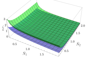
Figure 1: (Color Online) Separability surface $\mathcal{S}$ (bottom) and Classicality surface $\mathcal{P}$ (top). States either on or above $\mathcal{S}$ are separable while states either on or above $\mathcal{P}$ are classical. Between $\mathcal{S}$ and $\mathcal{P}$ there are classical and nonclassical separable states. Bellow $\mathcal{S}$, there are separable and entangled states. The divergence of both functions for $\bar{N}_{1}\to 0$ and for $\bar{N}_{2}\to 0$ are not shown in this plot.

To understand the sufficiency of the results for the system in consideration, as a consequence of the fact that ${\bf\Gamma}\neq{\bf\Gamma}^{\!\top}$, we will explore the separability and classicality criteria directly applying both to the CM of the steady-state. Using Eqs. (42), we are able to obtain analytically the solution ${\bf V}={\bf P}({\bf\Gamma},{\bf D})$ using (12) or solving algebraically the LE $\lfloor{\bf V},{\bf\Gamma},{\bf D}\rceil$. For simplicity and without loss of generality, we choose $\bar{N}_{1}=\bar{N}_{2}=\bar{N}$ and the solution is

$${\bf V} =(2\bar{N}+1)\mathsf{I}_{4}\,+$$ (48)

$$\frac{(2\bar{N}+1)\kappa}{\zeta^{2}+4\omega(\omega+\kappa)}\left[\begin{array}[]{cc}\omega&\tfrac{1}{2}\zeta\\ \tfrac{1}{2}\zeta&(\omega+\kappa)\end{array}\right]\!\otimes\!\left[\!\begin{array}[]{rr}-1&1\\ 1&-1\end{array}\!\right].$$

The steady-state is classical if and only if the above CM obeys (17), or working out its eigenvalues, if and only if

$$\frac{\zeta}{\kappa}\geq\mathcal{P}^{\prime}(\bar{N}):=\sqrt{\frac{1}{4\bar{N}^{2}}-\left(\frac{2\omega}{\kappa}+1\right)^{2}}.$$ (49)

As for separability, the steady state will be separable if and only if the condition (21) is satisfied, which reads as

$$\frac{\zeta}{\kappa}\geq\mathcal{S}^{\prime}(\bar{N}):=\sqrt{\frac{1}{16\bar{N}^{2}(\bar{N}+1)^{2}}-\left(\frac{2\omega}{\kappa}+1\right)^{2}}.$$ (50)

In Fig. 2, the two functions representing the necessary and sufficient conditions in Eqs. (49) and (50) are shown. We also compare them with the two sufficient conditions (45) and (47), already plotted in Fig. 1. It is clear that, for the system in question, even if the sufficient criteria become tighter for smaller values of $\bar{N}$, they are in general unable to determine whether a state is entangled or nonclassical.

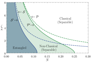
Figure 2: (Color Online) Necessary and sufficient conditions for classicality and for separability of the steady-state. We show the functions $\mathcal{P}^{\prime}(\bar{N})$ in (49) and $\mathcal{S}^{\prime}(\bar{N})$ in (50), as indicated in the graph. The regions limited by these two functions indicates the nature of the steady-state. We also plot the functions $\mathcal{S}(\bar{N},\bar{N})$ in (45) and $\mathcal{P}(\bar{N},\bar{N})$ in (47) as dashed curves, see Fig. 1. In this plot $\omega/\kappa=0.5$.

For the Gaussian-steering property, we also consider the case $\bar{N}_{1}=\bar{N}_{2}=\bar{N}$ and the sufficient condition is determined by calculating the matrix ${\bf D}_{[i{\bf\Pi}_{k}]}$ [the matrix ${\bf\Pi}_{k}$ is defined in (24), and here ${n_{1}}={n_{2}}=1$], which has the eigenvalues

$$\!\!\!\!\!\!{\rm Spec}_{\mathbb{R}}({\bf D}_{[i{\bf\Pi}_{1}]})={\rm Spec}_{\mathbb{R}}({\bf D}_{[i{\bf\Pi}_{2}]})=$$

$$\!\!\!\!\!\!\left\{(2\bar{N}+1),\zeta(2\bar{N}+1)\pm\sqrt{4\zeta^{2}+\kappa^{2}}\right\}.$$ (51)

The steady-state will be non-Gaussian steerable with respect to both partitions if $\zeta/\kappa\geq[4(2\bar{N}+1)^{2}+4]^{-1/2}$.

V.2 Two oscillators interacting with thermal baths in RWA

Let us consider the same system as before, but with the Hamiltonian

$${\bf H}=\left[\begin{array}[]{cc}\varpi_{1}&\Omega\\ \Omega&\varpi_{2}\end{array}\right]\oplus\left[\begin{array}[]{cc}\varpi_{1}&\Omega\\ \Omega&\varpi_{2}\end{array}\right].$$ (52)

This Hamiltonian is derived from the one in Eq.(39) by applying a rotating wave approximation (RWA). The procedure and the validity of this result are carefully discussed in the Appendix of Ref.nicacio2 , as well as the relation among the coupling constant $\Omega$ in Eq.(52) with the parameters in Eq.(39), see footnote2 for details. Considering also the same structure for the reservoirs in (41), one finds

$${\bf\Gamma}=\left[\begin{array}[]{cccc}-\tfrac{\zeta_{1}}{2}&0&\varpi_{1}&\Omega\\ 0&-\tfrac{\zeta_{2}}{2}&\Omega&\varpi_{2}\\ -\varpi_{1}&-\Omega&-\tfrac{\zeta_{1}}{2}&0\\ -\Omega&-\varpi_{2}&0&-\tfrac{\zeta_{2}}{2}\end{array}\right],$$ (53)

which is AS with eigenvalues

$$\!\!\!{\rm Spec}_{\mathbb{C}}({\bf\Gamma})\!=\!\left\{-\tfrac{\zeta_{1}+\zeta_{2}}{4}\pm\tfrac{1}{4}\sqrt{(\zeta_{1}-\zeta_{2})^{2}-4\Omega^{2}}\pm i\varpi\right\},$$ (54)

where we used $\varpi_{1}=\varpi_{2}=:\varpi$. Note that $\bf\Gamma$ in (53) and $\mathbf{D}$ in (42) are invariant under a rotation by $\mathsf{J}\in{\rm K}(2)$. Following Prop.3, the steady-state CM for this system will also be, i.e., $\mathbf{V}=\mathsf{J}\mathbf{V}\!\mathsf{J}^{\!\top}$, which means that position-momentum correlations are antisymmetric and position-position correlations are equal to momentum-momentum correlations. This symmetry help us to solve algebraically the LE (9), obtaining assadian

$${\bf V}=\left[\begin{array}[]{cccc}v_{1}&0&0&v_{14}\\ 0&v_{2}&-v_{14}&0\\ 0&-v_{14}&v_{1}&0\\ v_{14}&0&0&v_{2}\\ \end{array}\right],$$ (55)

with

$$v_{1} = 2\frac{\zeta_{1}\bar{N}_{1}+\zeta_{2}\bar{N}_{2}}{\zeta_{1}+\zeta_{2}}+\frac{2(\bar{N}_{1}-\bar{N}_{2})\zeta_{1}\zeta_{2}^{2}}{(\zeta_{1}+\zeta_{2})(4\Omega^{2}+\zeta_{1}\zeta_{2})}+1,$$

$$v_{2} = 2\frac{\zeta_{1}\bar{N}_{1}+\zeta_{2}\bar{N}_{2}}{\zeta_{1}+\zeta_{2}}+\frac{2(\bar{N}_{2}-\bar{N}_{1})\zeta_{1}^{2}\zeta_{2}}{(\zeta_{1}+\zeta_{2})(4\Omega^{2}+\zeta_{1}\zeta_{2})}+1,$$

$$v_{14} = \frac{4\zeta_{1}\zeta_{2}\Omega(\bar{N}_{2}-\bar{N}_{1})}{(\zeta_{1}+\zeta_{2})(\zeta_{1}\zeta_{2}+4\Omega^{2})}.$$ (56)

Note that, if $\zeta_{2}=0$, then ${\bf V}=(2\bar{N}_{1}+1)\mathsf{I}_{4}$, which has a simple structure, but it can not be simply retrieved by symmetries of $\bf\Gamma$ and $\bf D$.

The simple form of (55) can be used to explicitly analyze the results in conditions in (18). Considering for simplicity $\zeta_{1}=\zeta_{2}=\zeta$, the (doubly degenerate) spectrum of (55) is

$${\rm Spec}_{\mathbb{R}}({\bf V})=\left\{\bar{N}_{1}+\bar{N}_{2}+1\pm\frac{(\bar{N}_{1}-\bar{N}_{2})}{\sqrt{1+4\Omega^{2}/\zeta^{2}}}\right\}.$$ (57)

From this, it is easy to see that the state (55) is classical for any values of the parameters, since ${\bf V}-\mathsf{I}_{4}\geq 0$. On the other hand, let us calculate

$${\rm Spec}_{\mathbb{R}}({\bf D}_{[-\mathsf{I}]})=\left\{2\zeta\bar{N}_{1},2\zeta\bar{N}_{2}\right\},$$ (58)

which is non-negative for any value of $\bar{N}_{1}$ and $\bar{N}_{2}$. The statement in (18) thus tells us that all steady-states of this system belong to the set of classical states, which was already found by means of Eq.(57).

V.3 Cascaded OPO

Consider an optical parametric oscillator (OPO) coupled to the vacuum field koga . The Hamiltonian is written as $\hat{H}=i\hbar\epsilon({\hat{a}^{\dagger 2}}-{\hat{a}}^{2})/4$, where $\epsilon\geq 0$ denotes the effective pump intensity. The coupling with the vacuum is described by the operator $\hat{L}=\sqrt{\hbar\kappa}\hat{a}$, where $\kappa>0$ is the damping cavity rate.

With the help of Eqs. (4), (6), (7), and (10), one readily reaches

$${\bf\Gamma}=\left[\begin{array}[]{cc}\frac{1}{2}(\epsilon-\kappa)&0\\ 0&-\frac{1}{2}(\epsilon+\kappa)\end{array}\right],\,\,\,{\bf D}=\kappa\,\mathsf{I}_{2}.$$ (59)

The matrix $\bf\Gamma={\bf\Gamma}^{\!\top}$ will be AS in so far as $\kappa>\epsilon$. Also, ${\bf D}>0$, once $\kappa>0$. Following the statement in (19), since $\widetilde{\bf D}_{[i\mathsf{J}^{\!\top_{\!\!2}}]}={\rm Diag}\left(\epsilon,-\epsilon\right)$, the steady-state will be nonclassical if $\epsilon\neq 0$ and will be classical only if $\epsilon=0$. The LE is trivially solved to give the CM of the steady-state:

$${\bf V}={\rm Diag}[\kappa/(\kappa-\epsilon),\kappa/(\kappa+\epsilon)],$$ (60)

which is a squeezed thermal state and corresponds to the coherent-state solution in koga if $\epsilon=0$.

For a cascaded OPO koga , the system is described by the Hamiltonian $\hat{H}=\hat{H}_{1}+\hat{H}_{2}+\frac{1}{2i}(\hat{L}_{1}^{\dagger}\hat{L}_{2}-\hat{L}_{2}^{\dagger}\hat{L}_{1})$ with $\hat{H}_{j}=i\hbar\epsilon_{j}({\hat{a}_{j}^{\dagger 2}}-{\hat{a}_{j}}^{2})/4$ and $\hat{L}_{j}=\sqrt{\hbar\kappa}\hat{a}_{j}$. The coupling of the system with the intracavity vacuum is represented by $\hat{L}=\hat{L}_{1}+\hat{L}_{2}$. Under these circumstances we write

$${\bf D}=\left[\begin{array}[]{cc}\kappa&\kappa\\ \kappa&\kappa\end{array}\right]\oplus\left[\begin{array}[]{cc}\kappa&\kappa\\ \kappa&\kappa\end{array}\right],$$ (61)

and

$${\bf\Gamma}=\left[\!\!\begin{array}[]{cc}\frac{\epsilon_{1}-\kappa}{2}&0\\ -\kappa&\frac{\epsilon_{2}-\kappa}{2}\end{array}\!\!\right]\!\oplus\!\left[\!\!\begin{array}[]{cc}-\tfrac{\epsilon_{1}+\kappa}{2}&0\\ -\kappa&-\tfrac{\epsilon_{2}+\kappa}{2}\end{array}\!\!\right]$$ (62)

with spectrum given by

$${\rm Spec}({\bf\Gamma})=\left\{-\tfrac{1}{2}(\kappa\pm\epsilon_{1}),-\tfrac{1}{2}(\kappa\pm\epsilon_{2})\right\}.$$ (63)

Note that ${\bf\Gamma}\neq{\bf\Gamma}^{\!\top}$ is AS if $\kappa>\max\{|\epsilon_{1}|,|\epsilon_{2}|\}$. Now the eigenvalues of ${\bf D}_{[i\mathsf{J}^{\!\top_{\!\!2}}]}$ in (22) can be calculated, yielding

$${\rm Spec}_{\mathbb{R}}({\bf D}_{[i\mathsf{J}^{\!\top_{\!\!2}}]})=\{(1\pm\sqrt{5})\kappa,2\kappa,0\},$$ (64)

which shows that the state will be always entangled following Corol.1. The same arguments can be applied to determine the Gaussian steerability. Calculating the matrix ${\bf D}_{[i{\bf\Pi}_{k}]}$ [the matrix ${\bf\Pi}_{k}$ is defined in (24), and here ${n_{1}}={n_{2}}=1$], which has the eigenvalues

$${\rm Spec}_{\mathbb{R}}({\bf D}_{[i{\bf\Pi}_{1}]}) =\left\{(1\pm\sqrt{5})\frac{\kappa}{2},(3\pm\sqrt{5})\frac{\kappa}{2}\right\},$$ (65)

$${\rm Spec}_{\mathbb{R}}({\bf D}_{[i{\bf\Pi}_{2}]}) =\left\{(3\pm\sqrt{17})\frac{\kappa}{2},k,0\right\}.$$

From these, one concludes that the state will be always Gaussian steerable with respect to both modes since these spectra is nonpositive.

Following Prop.3, the CM of the steady-state of the cascaded OPO will have the symmetry induced by (26), and reads

$${\bf V}=\left[\begin{array}[]{cc}\frac{k}{k-\epsilon_{1}}&-\frac{2\kappa\epsilon_{1}}{g_{-}}\\ -\frac{2\kappa\epsilon_{1}}{g_{-}}&-\frac{\kappa h_{+}}{g_{-}}\end{array}\right]\oplus\left[\begin{array}[]{cc}\frac{k}{k+\epsilon_{1}}&\frac{2\kappa\epsilon_{1}}{g_{+}}\\ \frac{2\kappa\epsilon_{1}}{g_{+}}&\frac{\kappa h_{-}}{g_{+}}\end{array}\right],$$ (66)

where we have defined

$$g_{\pm} = (\epsilon_{1}+\epsilon_{2}\pm 2\kappa)(\epsilon_{1}\pm\kappa),$$

$$h_{\pm} = (\epsilon_{1}^{2}+\epsilon_{1}\epsilon_{2}\pm\epsilon_{1}\kappa+2\kappa^{2}\mp\kappa\epsilon_{2})(\epsilon_{2}\mp k)^{-1}.$$

V.4 OPO and Thermal Baths

Consider the Hamiltonian dynamics of two particles described by

$$\hat{H}=\frac{\epsilon}{4}{\boldsymbol{\{}}\hat{q}_{1},\hat{p}_{1}{\boldsymbol{\}}}_{\!+}+\frac{\epsilon}{4}{\boldsymbol{\{}}\hat{q}_{2},\hat{p}_{2}{\boldsymbol{\}}}_{\!+}+\frac{\kappa}{2}(\hat{q}_{2}\hat{p}_{1}+\hat{p}_{2}\hat{q}_{1}).$$ (67)

This Hamiltonian is similar to the one in the previous example, it is basically the Hamiltonian of the cascaded OPO with a phase change wiseman . If the particles are in contact with the thermal baths, as in (40), the dynamical matrices become

$${\bf\Gamma}={{\bf\Gamma}^{\!\top}}=\tfrac{1}{2}\!\left[\!\!\begin{array}[]{cc}\epsilon-\zeta&k\\ k&\epsilon-\zeta\end{array}\!\!\right]\!\oplus\tfrac{1}{2}\!\left[\!\!\begin{array}[]{cc}-(\epsilon+\zeta)&k\\ k&-(\epsilon+\zeta)\end{array}\!\!\right],$$ (68)

and $\bf D$ is as in (42), and now we are considering $\bar{N}_{1}=\bar{N}_{2}=\bar{N}$ and $\zeta_{1}=\zeta_{2}=\zeta$. The eigenvalues of $\bf\Gamma$ are

$${\rm Spec}({\bf\Gamma})=\left\{-\tfrac{1}{2}\zeta\pm\tfrac{1}{2}(\epsilon+\kappa),-\tfrac{1}{2}\zeta\pm\tfrac{1}{2}(\epsilon-\kappa)\right\},$$ (69)

and it will be AS if $\zeta>\epsilon+\kappa$. The eigenvalues of ${\bf D}_{[-\mathsf{I}]}$ in (19) are

$${\rm Spec}_{\mathbb{R}}({\bf D}_{[-\mathsf{I}]})=\left\{2\zeta\bar{N}\pm(\epsilon+\kappa),2\zeta\bar{N}\pm(\epsilon-\kappa)\right\},$$ (70)

which shows that the state will be classical if and only if $2\zeta\bar{N}\geq(\epsilon+\kappa)$. The eigenvalues of $\widetilde{\bf D}_{[i\mathsf{J}^{\!\top_{\!\!2}}]}$ in (22b) are

$${\rm Spec}_{\mathbb{R}}(\widetilde{\bf D}_{[i\mathsf{J}^{\!\top_{\!\!2}}]})=\{2\zeta\bar{N}\pm\kappa,2\zeta(\bar{N}+1)\pm\kappa\},$$ (71)

and the steady-state will be entangled if and only if $2\zeta\bar{N}<\kappa$. In the interval $(\epsilon+\kappa)>2\zeta\bar{N}\geq\kappa$, the state is nonclassical and separable. The steerability of the state is determined by

$$\!\!\!\!\!\!{\rm Spec}_{\mathbb{R}}(\widetilde{\bf D}_{[i{\bf\Pi}_{1}]})={\rm Spec}_{\mathbb{R}}(\widetilde{\bf D}_{[i{\bf\Pi}_{2}]})=$$

$$\!\!\!\!\!\!\left\{(2\bar{N}+\tfrac{1}{2})\zeta\pm\sqrt{\zeta^{2}+\kappa^{2}},(2\bar{N}+\tfrac{3}{2})\zeta\pm\sqrt{\zeta^{2}+\kappa^{2}}\right\}.$$ (72)

As a consequence of the chosen parameters, the steady state is symmetric with respect to the steerings of both partitions. This is state is steerable if and only if $(2\bar{N}+\tfrac{1}{2})\zeta<\sqrt{\zeta^{2}+\kappa^{2}}$.

VI Engineering Steady-States

The unavoidable influence of uncontrollable degrees of freedom are usually responsible for losses of the quantumness of a system through the procedure called decoherence. However, a steady-state with a desired quantum property can be produced by controlling the parameters of the system and of the environmental action. As the examples of the last section, systems of bosonic degrees of freedom have been extensively studied in what concerns entanglement generation tan ; houhou , production of pure states koga ; ikeda , and engineering of graph states koga ; houhou . On the experimental side, realizations of these techniques in the context of atomic ensembles were already performed krauter .

To develop a simple theoretical engineering-state method for bosonic degrees of freedom, we will use the results provided by the Williamson theorem williamson ; gosson ; simon :

Theorem 1 (Williamson).

Let $\mathbf{M}\in{\rm Mat}(2n,\mathbb{R})$ be a positive definite matrix: $\mathbf{M}=\mathbf{M}^{\top}>0$. This matrix can be diagonalized by a symplectic congruence, i.e., there exists $\mathsf{S}\in{\rm Sp}(2n,\mathbb{R})$ such that

$$\mathsf{S}\mathbf{M}\mathsf{S}^{\top}={\rm Diag}(\mu_{1},...,\mu_{n},\mu_{1},...,\mu_{n})=:{\bf\Lambda},$$ (73)

where $\mu_{j}\geq\mu_{k}>0\,\,\,\text{for}\,\,\,j>k.$

The double-paired ordered set (or the diagonal matrix) $\bf\Lambda$ is called symplectic spectrum of $\mathbf{M}$, and $\mu_{k}$ are its symplectic eigenvalues (SE). These can be found from the (Euclidean) eigenvalues of $\mathsf{J}\mathbf{M}$ gosson , which turn out to be

$${\rm Spec_{\mathbb{C}}}(\mathsf{J}\mathbf{M})={\rm Diag}(i\mu_{1},...,i\mu_{n},-i\mu_{1},...,-i\mu_{n}).$$ (74)

Suppose one wants to design a reservoir structure able to produce a steady-state (with $n$ degrees of freedom) described by a $2n\times 2n$ CM ${\bf V}^{\prime}$. If one identifies this CM with $\bf M$ in (73), the first step is to find a suitable LE able to produce its corresponding symplectic spectrum $\bf\Lambda$ as a solution, i.e., its is necessary to find matrices ${\bf\Gamma}^{\prime}$ and ${\bf D}^{\prime}$ satisfying the LE $\lfloor{\bf\Lambda},{\bf\Gamma}^{\prime},{\bf D}^{\prime}\rceil$. Assuming that it is possible to design a system-reservoir structure with this LE, one applies the symplectic covariance (29) to it and finds

$$\left\lfloor{\bf V}^{\prime},\mathsf{S}^{-1}{\bf\Gamma}^{\prime}\mathsf{S},\mathsf{S}^{-1}{\bf D}^{\prime}\mathsf{S}^{-\top}\right\rceil,$$ (75)

which, by Eq.(73), is the LE with solution ${\bf V}^{\prime}=\mathsf{S}^{-1}{\bf\Lambda}\mathsf{S}^{-\top}$. Reservoir engineering can then be realized by finding some convenient matrix $\bf\Lambda$ and a system-reservoir structure suitable to the unitary transformations, as in (30). Following Eq.(29), the engineered Hamiltonian and Lindblad operators will be, respectively, such that ${\bf H}^{\prime}={\sf S}^{\!\top}\!{\bf H}{\sf S}$ and $\lambda^{\prime}={\sf S}^{-1}{\lambda}$.

A peculiar example using (75) appears when one is able to produce a reservoir structure such that ${\bf D}^{\prime}=\beta\bf\Lambda$ and ${\bf\Gamma}^{\prime}=-\beta\mathsf{I}_{2n}$ with $\beta>0$, thus the use of (73) gives that $\left\lfloor{\bf V}^{\prime},-\beta\mathsf{I}_{2n},\beta{\bf V}^{\prime}\right\rceil$. This shows that a Lindblad equation with ${\bf\Upsilon}=\tfrac{1}{2}\beta{\bf V}^{\prime}+i\beta\mathsf{I}_{2n}$ [see Eq.(7)] will have a steady-state automatically given by a Gaussian with CM ${\bf V}^{\prime}$.

In fact, the matrix $\bf\Lambda$ in (73) is like the CM in (38), thus any $\bf\Gamma^{\prime}$ as in (36) and $\bf D^{\prime}$ as in (37), which are invariants under the local rotations in (35), are appropriate to the first step of the method. It is noticeable that not all reservoir structure are suitable to produce a diagonal matrix $\bf\Lambda$ as a CM of a steady-state, since it can not have the desired invariant structure for performing the first step. However, it is still possible to use the covariance relation (29) to design a specific steady-state from a known simple steady-state of some system, one of these cases (the OPO in Sec. V.3) will be analyzed at the end of this section.

The special condition presented in Corol.3 can be used to engineer a specific and important class of states. Explicitly, we will use the relation (29) to generate a state with CM ${\bf V}^{\prime}=\alpha\mathsf{SS}^{\!\top}$, where $\mathsf{S}\in{\rm Sp}(2n,\mathbb{R})$ and $\alpha\geq 1$. In other words, we want to know which matrices $\bf\Gamma_{\rm p}$ AS and ${\bf D}_{\rm p}\geq 0$ are necessary to construct a LE with the solution given by the desired CM. Note that the above-mentioned CM represents a pure state if and only if $\alpha=1$ koga ; simon ; gosson .

As stated in Corol.3, the $n$-mode Gibbs state with ${\bf V}=\alpha\mathsf{I}_{2n}$ is generated by any LE of the form $\lfloor{\bf V},{\bf\Gamma}^{\prime},-\alpha({\bf\Gamma}^{\prime}+{\bf\Gamma}^{\prime\!\top})\rceil$, for all matrices $\bf\Gamma^{\prime}$ AS such that $({\bf\Gamma}^{\prime}+{\bf\Gamma}^{\prime\!\top})\leq 0$. Using the relation (29), we are able to obtain a covariant LE $\lfloor{\bf V}^{\prime},{\bf\Gamma}_{\rm p},{\bf D}_{\rm p}\rceil$ with

$$\!\!\!{\bf V}^{\prime}=\alpha\mathsf{SS}^{\!\top},\,\,{\bf\Gamma}_{\rm p}=\mathsf{S}{\bf\Gamma}^{\prime}\mathsf{S}^{-1},\,\,{\bf D}_{\rm p}=-\alpha\,\mathsf{S}({\bf\Gamma}^{\prime}+{\bf\Gamma}^{\prime\!\top})\mathsf{S}^{\!\top}.$$ (76)

It is interesting to note that, recalling Corol.3, the value of $\alpha$ only depends on the reservoir structure (it does not depend on the Hamiltonian of the system) used to prepare the initial state ${\bf V}=\alpha\mathsf{I}_{2n}$; conveniently the Hamiltonian at this stage can be taken as zero. Another remarkable fact is that any one-mode Gaussian state $(n=1)$ is included in the scheme provided by Eq.(76): these states have a CM written as ${\bf V}^{\prime}$ in (76) with $\alpha=\mu_{1}\geq 1$ and $\mathsf{S}\in{\rm Sp}(2,\mathbb{R})$, as a consequence of the Williamson theorem.

In koga , the authors established specific conditions for a system to be driven to a pure steady-state when evolving under the LME subjected to the restrictions in (4). Equation (76) with $\alpha=1$ constitutes a simple connection with some of their results.

Examples

Two Mode Thermal Squeezed States (TMTSS).

Consider the following CM

$${\bf V}^{\prime}=(2\bar{n}+1)\mathsf{S}_{r}\mathsf{S}_{r}^{\!\top},$$ (77)

with

$${\mathsf{S}_{r}}:=\left[\left(\!\begin{array}[]{cc}\cosh r&\sinh r\\ \sinh r&\cosh r\\ \end{array}\!\right)\!\oplus\!\left(\!\begin{array}[]{cc}\cosh r&-\sinh r\\ -\sinh r&\cosh r\\ \end{array}\!\!\right)\right],$$ (78)

where $r\geq 0$ is the squeezing parameter and $\bar{n}\geq 0$ is the mean number of thermal photons of both modes. Note that ${\mathsf{S}_{r}}\in{\rm Sp}(4,\mathbb{R})$. Following the criteria (21) and (24), the state in (77) will be respectively entangled iff $r>{\rm ln}(2\bar{n}+1)$ and steerable iff $r>{\rm cosh}^{-1}(2\bar{n}+1)$.

If one wants to engineer a reservoir with the steady-state given in (77), it is possible to apply the scheme in Eq.(76). For this purpose, one needs a reservoir structure able to produce a steady-state of the form ${\bf V}=\alpha\mathsf{I}_{2n}$ with $\alpha=(2\bar{n}+1)$. An example of a system with this steady-state is the one in Sec.V.2 with $\bar{N}_{1}=\bar{N}_{2}$. The system in Sec.V.1 can also be used to this end, but now, besides the condition $\bar{N}_{1}=\bar{N}_{2}$, one needs to take $\kappa=0$ — this condition is necessary to guarantee that ${\bf\Gamma}+{\bf\Gamma}^{\!\top}\leq 0$, as required in Corol.3. Recalling that the Hamiltonian dynamics does not affect the value of $\alpha$ in (76), one can use either $\omega_{1}=\omega_{2}=\kappa=0$ and $\zeta_{1}=\zeta_{2}:=\zeta$ in (42), or $\varpi_{1}=\varpi_{2}=\Omega=0$ and $\zeta_{1}=\zeta_{2}:=\zeta$ in (53) to obtain a reservoir structure with ${\bf\Gamma}^{\prime}=-\frac{\zeta}{2}\mathsf{I}_{4}$ and ${\bf D}^{\prime}=(2\bar{n}+1)\zeta\,\mathsf{I}_{4}$. This structure produces the steady-state ${\bf V}=(2\bar{n}+1)\mathsf{I}_{2n}$.

Now, one needs to apply the covariance relation (76) and determine the engineered reservoir with matrices ${\bf\Gamma}_{\rm p}$ and ${\bf D}_{\rm p}$ through the symplectic matrix (78), i.e.,

$${\bf\Gamma}_{\rm p}=-\frac{\zeta}{2}\mathsf{I}_{4},\,\,\,{\bf D}_{\rm p}=(2\bar{n}+1)\zeta\,\mathsf{S}_{r}\mathsf{S}_{r}^{\!\top}.$$ (79)

From Eq.(29), one can see that $\lambda^{\prime}=\mathsf{S}_{r}\lambda$, and the Lindblad operators in (4) for $\lambda^{\prime}$ are characteristics of a squeezed thermal bath.

OPO Steady-States.

The steady-state in (66) is a pure steady-state iff $\epsilon_{1}=-\epsilon_{2}$ koga . Under these conditions and if we define $\epsilon:=\sqrt{(\kappa+\epsilon_{2})/(\kappa-\epsilon_{2})}$, the CM of this steady-state is written as

$${\bf V}^{\prime}=\mathsf{S}_{\rm p}\mathsf{S}_{\rm p}^{\top},\,\,\,{\mathsf{S}_{\rm p}}:=\left(\!\begin{array}[]{cc}\frac{1+\epsilon}{2}&\frac{1-\epsilon}{2}\\ \frac{1-\epsilon}{2}&\frac{1+\epsilon}{2}\end{array}\!\right)\oplus\left(\!\begin{array}[]{cc}\frac{1+\epsilon}{2\epsilon}&\frac{\epsilon-1}{2\epsilon}\\ \frac{\epsilon-1}{2\epsilon}&\frac{1+\epsilon}{2\epsilon}\end{array}\!\right),$$ (80)

which is entangled for any value of $\epsilon$. Obviously, if one wants to produce this pure state as a steady-state of an OPO, the only step is to produce an OPO satisfying the mentioned conditions. On the other side, it is not possible to produce it by using the covariance rules in (76) for an OPO, since Corol.3 requires ${\bf\Gamma}+{\bf\Gamma}^{\top}\geq 0$, which is not the case for $\bf\Gamma$ in (62) with $\epsilon_{1}=-\epsilon_{2}$.

By the Willianson theorem, the symplectic spectrum of the CM of the pure state in (80) is the identity matrix footnote3 . If one can choose suitable values of the parameters in (61) and (62) such that ${\bf\Gamma}^{\prime}$ and $\bf D^{\prime}$ satisfy the LE $\lfloor\mathsf{I}_{4},{\bf\Gamma}^{\prime},{\bf D}^{\prime}\rceil$, then Eq.(75) can be applied. In fact, this happens when $\epsilon_{1}=\epsilon_{2}=0$. Thus, preparing an OPO system such that this last condition holds, Eq.(75) becomes

$$\left\lfloor\mathsf{S}_{\rm p}\mathsf{S}_{\rm p}^{\top},\mathsf{S}_{\rm p}{\bf\Gamma}^{\prime}\mathsf{S}_{\rm p}^{-1},\mathsf{S}_{\rm p}{\bf D}^{\prime}\mathsf{S}_{\rm p}^{\top}\right\rceil.$$ (81)

with ${\bf D}^{\prime}$ as in (61) and

$${\bf\Gamma}^{\prime}=\left[\!\!\begin{array}[]{cc}-\frac{\kappa}{2}&0\\ -\kappa&-\frac{\kappa}{2}\end{array}\!\!\right]\!\oplus\!\left[\!\!\begin{array}[]{cc}-\tfrac{\kappa}{2}&0\\ -\kappa&-\tfrac{\kappa}{2}\end{array}\!\!\right].$$ (82)

Note that the matrices $\bf\Gamma^{\prime}$ and $\bf D^{\prime}$ in this example do not have the invariant structure in (35). Note also that the same pure state can be engineered by using thermal baths. The recipe for this case is just (79) but replacing $\mathsf{S}_{r}$ by $\mathsf{S}_{\rm p}$ and using $\bar{n}=0$.

An entangled and steerable (with respect to both partitions) mixed state can also be prepared by following the same recipe. Suppose that one wants to create the bellow state as a steady-state of an OPO-covariant-LE:

$${\bf V}^{\prime}={\mathsf{S}}_{\rm p}^{-1}{\bf\Lambda}{\mathsf{S}}_{\rm p}^{-\top},$$ (83)

with $\mathsf{S}_{\rm p}$ defined in (80) and

$${\bf\Lambda}={\rm Diag}\left[1,(1-\epsilon)^{-1},1,(1+\epsilon)^{-1}\right].$$ (84)

This matrix is the solution for the LE $\lfloor{\bf\Lambda},{\bf\Gamma}^{\prime},{\bf D}^{\prime}\rceil$ with $\bf D^{\prime}$ in (61) and $\bf\Gamma^{\prime}$ in (62) both with $\kappa=1$, $\epsilon_{1}=0$ and $\epsilon_{2}=\epsilon$. By the same recipe as before, the LE in (75) has the above $\bf V^{\prime}$ as solution if we replace $\mathsf{S}$ by $\mathsf{S}_{\rm p}$ and the mentioned matrices $\bf\Gamma^{\prime}$ and $\bf D^{\prime}$.

VII Final Remarks

Symmetries and properties of the Lyapunov equation were used to classify the features of the steady state of a LME with a quadratic Hamiltonian and linear Lindblad operators. The connection with the Lyapunov equation eases the characterization of the state, a task that is typically difficult when performed using the master equation directly.

For Gaussian steady-states, we focused on known bona-fide relations for the covariance matrix of a state. Specifically, we considered conditions for the classicality, separability, and steerability of Gaussian states. We remark, however, that the extension for any other bona-fide relation is straightforward and can be performed following the lines presented here. For instance, we can refer to the characterization of tripartite entanglement given in Ref. giedke . We also analyze the consequences for the covariance matrix of a steady-state when a transformation symmetry of the Lyapunov equation is performed.

We focused our examples on systems with one or two degrees of freedom, which has enabled us to compare the results of our corollaries with the results extracted directly from the covariance matrix of the system after solving the Lyapunov equation. However, our results are applicable to systems with a generic number of degrees of freedom. For large systems, in particular in the absence of symmetries, numerical solutions might be needed to find the covariance matrix of the steady-state; for instance, the systems considered in Ref. nicacio3 . In this situation, instabilities associated with the algorithms for solving Lyapunov equations may arise hammarling . The robustness of the analytical results shows the advantage with respect to either perturbations of the systems parameters or preparation imprecisions. In other words, our results are advantageous since one does not need to solve a Lyapunov equation to know some of the system properties or symmetries. In addition, our results are suitable for the engineering of (a reservoir leading to a specific) steady-state of a LME having suitable properties and symmetries.

Appendices

Appendix I: Notations and Definitions

Throughout the text we use some mathematical objects whose notations are defined here.

• ${\rm Mat}(m,\mathbb{K})$: set of all $m\times m$ square matrices over the field $\mathbb{K}$.

• ${\rm GL}(m,\mathbb{K}):=\{{\bf M}\in{\rm Mat}(m,\mathbb{K})|\det{\bf M}\neq 0\}$: General linear group over field $\mathbb{K}$.

• ${\rm Sp}(2m,\mathbb{R}):=\{{\mathsf{M}}\in{\rm Mat}(2m,\mathbb{R})|\mathsf{M}\mathsf{J}\mathsf{M}^{\top}=\mathsf{J}\}$: Real symplectic group.

• ${\rm O}(m):=\{M\in{\rm Mat}(m,\mathbb{R})|MM^{\top}=\mathsf{I}_{m}\}$: Real orthogonal group.

• $\mathsf{I}_{m}$: Identity matrix in ${\rm Mat}(m,\mathbb{K})$.

• ${\bf 0}_{m}$: Zero matrix in ${\rm Mat}(m,\mathbb{K})$.

• ${\rm Spec}_{\mathbb{K}}({\bf M}):=\{\nu_{1},...,\nu_{l}\}$ is the spectrum of ${\bf M}\in{\rm Mat}(m,\mathbb{K})$. It is the set of its eigenvalues $\nu_{k}\in\mathbb{K},\,\forall k$ and $l\leq m$.

• ${\bf M}^{\!\top}$: Transposition of $\bf M$;   ${\bf M}^{-\top}$: Inverse of $\bf M^{\!\top}$.

• ${\bf M}^{\ast}$: Complex conjugation of the elements of $\bf M$.

• ${\rm In}({\bf M}):=(n_{+},n_{0},n_{-})(\bf M)$: Inertia index, i.e., the triple containing the number of eigenvalues of ${\bf M}$ with positive ($n_{+}$), null ($n_{0}$) and negative ($n_{-}$) real part. N.B. if ${\bf M}\in{\rm Mat}(m,\mathbb{K})$, then $m=n_{+}+n_{0}+n_{-}$.

In what follows, ${\bf M}\in{\rm Mat}(m,\mathbb{K})$ and ${\bf M}={\bf M}^{\dagger}$:

• ${\bf M}>0$ (resp. ${\bf M}<0$): Positive (resp. negative) definiteness of ${\bf M}$, i.e., all its eigenvalues are positive (resp. negative).

• ${\bf M}\geq 0$ (resp. ${\bf M}\leq 0$): Positive (resp. negative) semidefiniteness of ${\bf M}$, i.e., all its eigenvalues are non-negative (resp. nonpositive). In this text, the statement ${\bf M}\geq 0$ (resp. ${\bf M}\leq 0$) means that $\bf M$ can, but not necessarily, have null eigenvalues. This is the same as say that the set of matrices such that ${\bf M}>0$ (resp. ${\bf M}<0$) is a subset of the ones satisfying ${\bf M}\geq 0$ (resp. ${\bf M}\leq 0$).

It is noteworthy that, following our definitions, the sum of two positive (resp. negative) semidefinite matrices is positive (resp. negative) semidefinite, i.e., the sum will have non-negative (resp. non-positive) eigenvalues. In addition, the sum of two positive (resp. negative) definite matrices is positive (resp. negative) definite.

Appendix II: On the P-Representability of States

Due to the absence of a proof in the literature, this appendix is devoted to prove that the necessary and sufficient condition for P-Representability of a $n$-mode Gaussian state is Eq.(17).

A quantum state $\hat{\rho}$ is P-representable, by definition, if it can be written as a convex and regular sum of coherent states through the Glauber-Sudarshan $P$-function sudarshan :

$$\hat{\rho}=\int\!P(\zeta)\,|\zeta\rangle\!\langle\zeta|\,d^{2n}\zeta,$$ (A-1)

where $\zeta\in\mathbb{R}^{2n}$ and $|\zeta\rangle$ is a coherent state.

The sufficient condition is proved in englert for two mode Gaussian states, i.e., $n=2$ in (A-1). The extension for any $n$-mode state (not only the Gaussians) follows the same recipe: using the definition of the CM (8) with the $\hat{\rho}$ in (A-1), Eq.(17) follows immediately.

To prove the necessary condition (only for Gaussian states), we choose two Gaussian states $\hat{\rho}$ and $\hat{\rho}_{0}$, with the respective CMs ${\bf V}$ and ${\bf V}_{0}$ such that ${\bf V}\geq{\bf V}_{0}$. These states can be related through a Gaussian noise channel caves :

$$\hat{\rho}=\frac{1}{(\pi\hbar)^{n}}\int^{+\infty}_{-\infty}\frac{{\rm e}^{-\frac{1}{\hbar}\zeta\cdot\Delta^{-1}\zeta}}{\sqrt{\rm Det\Delta}}\,\,\hat{T}_{\zeta}\hat{\rho}_{0}\hat{T}_{\zeta}^{\dagger}\,\,\,d^{2n}\zeta.$$ (A-2)

The operators $\hat{T}_{\zeta}$ are the Weyl displacement operators gosson , and $\Delta:={\bf V}-{\bf V}_{0}\geq 0$. Mathematically speaking, Eq.(A-2) express the very known fact that the convolution of two Gaussian functions is a Gaussian function. If we choose ${\bf V}_{0}=\mathsf{I}_{2n}$ and $\hat{\rho}_{0}$ as a vacuum state, the positive-semidefiniteness of $\Delta$ implies relation (17), as we should prove.

- (1) J.F. Poyatos, J.I. Cirac & P. Zoller, Quantum reservoir engineering with laser cooled trapped ions, Phys. Rev. Lett. 77, 4728 (1996), A.R.R. Carvalho, P. Milman, R.L. de Matos Filho & L. Davidovich, Decoherence, pointer engineering and quantum state protection (Modern Challenges in Quantum Optics, Springer, 2001). M.B. Plenio & S.F. Huelga, Entangled light from white noise, Phys. Rev. Lett. 88, 197901 (2002), arXiv:quant-ph/0110009. S. Diehl, A. Micheli, A. Kantian, B. Kraus, H.P. Büchler & P. Zoller, Quantum states and phases in driven open quantum systems with cold atoms, Nat. Phys. 4, 878 (2008), arXiv: 0803.1482 [quant-ph]; F. Verstraete, M.M. Wolf & J.I. Cirac, Quantum computation and quantum-state engineering driven by dissipation, Nat. Phys. 5, 633 (2009), arXiv:0803.1447 [quant-ph].
- (2) F. Ticozzi, S.G. Schirmer & X. Wang, Stabilizing Quantum States by Constructive Design of Open Quantum Dynamics, IEEE Trans. Autom. Cont. 55, 2901 (2010), arXiv:0911.4156 [quant-ph].
- (3) V.V. Albert & L. Jiang, Symmetries and conserved quantities in Lindblad master equations, Phys. Rev. A 89, 022118 (2014), arXiv:1310.1523 [quant-ph].
- (4) H.M. Wiseman & G.J. Milburn, Quantum Measurement and Control (Cambridge University Press, New York, 2009).
- (5) G. Lindblad, On the Generators of Quantum Dynamical Semigroups, Commun. Math. Phys. 48 (2), 119 (1976).
- (6) H.-P. Breuer & F. Petruccione, Theory of Open Quantum Systems (Oxford University Press, New York, 2002).
- (7) A good and extensive set of references for applications can be found in Ref.albert .
- (8) S. Lloyd & S.L. Braunstein, Quantum Computation over Continuous Variables, Phys. Rev. Lett. 82, 1784 (1999), arXiv: quant-ph/9810082.
- (9) G.E. Dullerud & F.G. Paganini, A Course in Robust Control Theory - A Convex Approach (Springer-Verlag, New York, 2000).
- (10) A.M. Lyapunov, The General Problem of Stability of Motion (Taylor & Francis, London, 1992).
- (11) K. Koga & N. Yamamoto, Dissipation-induced pure Gaussian state, Phys. Rev. A 85, 022103 (2012), arXiv:1103.5449 [quant-ph].
- (12) B.-G. Englert & K. Wódkiewicz, Separability of two-party Gaussian states, Phys. Rev. A 65, 054303 (2002). arXiv:quant-ph/0107131.
- (13) R. Simon, Peres-Horodecki Separability Criterion for Continuous Variable Systems, Phys. Rev. Lett. 84, 2726 (2000), arXiv:quant-ph/9909044.
- (14) R.F. Werner & M.M. Wolf, Bound Entangled Gaussian States, Phys. Rev. Lett. 86, 3658 (2001), arXiv:quant-ph/0009118.
- (15) H.M. Wiseman, S.J. Jones and A.C. Doherty, Steering, Entanglement, Nonlocality, and the Einstein-Podolsky-Rosen Paradox, Phys. Rev. Lett. 98, 140402 (2007), arXiv:0709.0390 [quant-ph].
- (16) F. Nicacio, R.N.P. Maia, F. Toscano & R.O. Vallejos, Phase space structure of generalized Gaussian cat states, Phys. Lett. A 374, 4385 (2010), arXiv:1002.2248 [quant-ph].
- (17) Our definition of the CM differs from the standard one simon and is related to the choice of the CCR . This convenience is to avoid some undesired multiplicative factors, e.g., for a pure state in our notation.
- (18) R. A. Horn & C. R. Johnson, Topics in Matrix Analysis (Cambridge University Press, New York, 1994).
- (19) R. Simon, N. Mukunda & B. Dutta, Quantum-noise matrix for multimode systems: invariance, squeezing, and normal forms, Phys. Rev. A 49, 1567 (1994).
- (20) M. de Gosson, Symplectic Geometry and Quantum Mechanics (Birkhäuser, Basel, series “Operator Theory: Advances and Applications”, 2006).
- (21) F. Nicacio and F. L. Semião, Coupled Harmonic Systems as Quantum Buses in Thermal Environments, J. Phys. A: Math. Theor. 49, 375303 (2016), arXiv:1601.07528 [quant-ph].
- (22) As stated in Ref.nicacio2 , if we consider the dynamics of Hamiltonian (39), move to an interaction picture with respect to the free oscillators evolutions with frequencies and , perform the RWA (discarding the fast oscillation terms) and back again to Schrödinger picture, we obtain Eq.(52) with and .
- (23) A. Asadian, D. Manzano, M. Tiersch & H.J. Briegel, Heat transport through lattices of quantum harmonic oscillators in arbitrary dimensions, Phys. Rev. E 87, 012109 (2013), arXiv:1204.0904 [quant-ph].
- (24) H. Tan, L.F. Buchmann, H. Seok & G. Li, Achieving steady-state entanglement of remote micromechanical oscillators by cascaded cavity coupling, Phys. Rev. A 87, 022318 (2013), arXiv:1210.2345 [quant-ph]; H. Tan, G. Li & P. Meystre, Dissipation-driven two mode mechanical squeezed states in optomechanical systems, Phys. Rev. A 87, 033829 (2013), arXiv:1301.5698 [quant-ph]; M.J. Woolley, A.A. Clerk Two-mode squeezed states in cavity optomechanics via engineering of a single reservoir, Phys. Rev. A 89, 063805 (2014), arXiv: 1404.2672 [quant-ph]; M. Abdi, M.J. Hartmann, Entangling the motion of two optically trapped objects via time-modulated driving fields, New J. Phys. 17, 013056 (2015), arXiv: 1408.3423 [quant-ph]; Y.-D. Wang & A.A. Clerk, Reservoir-engineered entanglement in optomechanical systems, Phys. Rev. Lett. 110, 253601 (2013), arXiv:1301.5553 [cond mat. mes-hall].
- (25) O. Houhou, H. Aissaoui, A. Ferraro, Generation of cluster states in optomechanical quantum systems, Phys. Rev. A 92, 063843 (2015), arXiv:1508.02264 [quant-ph].
- (26) Y. Ikeda & N. Yamamoto, Deterministic generation of Gaussian pure state in quasi-local dissipative system, Phys. Rev. A 87, 033802 (2013), arXiv:1211.5788 [quant-ph].
- (27) H. Krauter, C.A. Muschik, K. Jensen, W. Wasilewski, J.M. Petersen, J.I. Cirac & E.S. Polzik, Entanglement generated by dissipation and steady state entanglement of two macroscopic objects, Phys. Rev. Lett. 107, 080503 (2011), arXiv:1006.4344 [quant-ph]; C.A. Muschik, E.S. Polzik & J.I. Cirac, Dissipatively driven entanglement of two macroscopic atomic ensembles, Phys. Rev. A 83, 052312 (2011), arXiv:1007.2209 [quant-ph]; C.A. Muschik, H. Krauter, K. Jensen, J.M. Petersen, J.I. Cirac & E.S. Polzik, Robust entanglement generation by reservoir engineering, J. Phys. B: At. Mol. Opt. Phys. 45, 124021 (2012), arXiv:1203.4785 [quant-ph].
- (28) J. Williamson, An algebraic problem involving the involutory integrals of linear dynamical systems, Amer. J. Math. 58, 141 (1936).
- (29) This affirmation is true for any pure states, i.e., for any CM of the form , .
- (30) G. Giedke, B. Kraus, M. Lewenstein, & J.I. Cirac, Separability properties of three-mode Gaussian states, Phys. Rev. A 64, 052303 (2001), arXiv:quant-ph/0103137.
- (31) F. Nicacio, A. Ferraro, A. Imparato, M. Paternostro & F.L. Semião, Thermal transport in out of equilibrium quantum harmonic chains, Phys. Rev. E 91, 042116 (2015), arXiv:1410. 7604 [quant-ph].
- (32) S.J. Hammarling, Numerical Solution of the Stable, Non-negative Definite Lyapunov Equation Lyapunov Equation, IMA J. Numer. Anal. 2, 303 (1982); P. Benner, J.-R. Li & T. Penzl, Numerical solution of large-scale Lyapunov equations, Riccati equations, and linear-quadratic optimal control problems, Numer. Linear Algebra Appl. 15, 755 (2008).
- (33) E.C.G. Sudarshan, Equivalence of Semiclassical and Quantum Mechanical Descriptions of Statistical Light Beams, Phys. Rev. Lett. 10, 277(1963); R.J. Glauber, Coherent and Incoherent States of the Radiation Field, Phys. Rev. 131, 2766 (1963).
- (34) C.M. Caves & K. Wodkiewicz, Fidelity of Gaussian Channels, Open Sys. Inf. Dyn. 11, 309 (2004), arXiv:quant-ph/0409063.