THE APPROXIMATION OF PARABOLIC EQUATIONS INVOLVING FRACTIONAL POWERS OF ELLIPTIC OPERATORS

Abstract.

We study the numerical approximation of a time dependent equation involving fractional powers of an elliptic operator $L$ defined to be the unbounded operator associated with a Hermitian, coercive and bounded sesquilinear form on $H^{1}_{0}(\Omega)$. The time dependent solution $u(x,t)$ is represented as a Dunford Taylor integral along a contour in the complex plane.

The contour integrals are approximated using sinc quadratures. In the case of homogeneous right-hand-sides and initial value $v$, the approximation results in a linear combination of functions $(z_{q}I-L)^{-1}v\in H^{1}_{0}(\Omega)$ for a finite number of quadrature points $z_{q}$ lying along the contour. In turn, these quantities are approximated using complex valued continuous piecewise linear finite elements.

Our main result provides $L^{2}(\Omega)$ error estimates between the solution $u(\cdot,t)$ and its final approximation. Numerical results illustrating the behavior of the algorithms are provided.

1. Introduction

We consider the approximation of parabolic equations where the elliptic part is given by a fractional power of an elliptic boundary value operator. This is a prototype for time dependent equations with integral or nonlocal operators and has numerous applications [9, 10, 11, 1, 3]. For example, a non-local operator results from replacing Brownian diffusion with Levy-diffusion. When the spatial domain is bounded, the fractional powers $L^{\beta}$ can be defined in terms of Fourier series, namely,

(1.1) $$L^{\beta}v=\sum_{j=1}^{\infty}(v,\psi_{j})\lambda_{j}^{\beta}\psi_{j}.$$

Here $(\cdot,\cdot)$ denotes the Hermitian $L^{2}(\Omega)$ inner product and $\{\psi_{j}\}$ is an $L^{2}(\Omega)$-orthonormal basis of eigenfunctions of $L$ with eigenvalues $\{\lambda_{j}\}$. An alternate, yet equivalent, formulation can be found in [18, 21] for general regularly accretive operators $L$, see also [4].

In this paper, we focus on a bounded domain problem where $\mathbb{R}^{d}$ is replaced by a bounded domain $\Omega\subset\mathbb{R}^{d}$ and for $T>0$, the targeted function $u:\Omega\times[0,T]\rightarrow\mathbb{R}$ satisfies

(1.2) $$\left\{\begin{aligned} u_{t}+L^{\beta}u=f,&\qquad\text{in }\Omega\times(0,T),\\ u=0,&\qquad\text{on }\partial\Omega\times(0,T),\\ u(t=0)=v,&\qquad\text{on }\Omega.\\ \end{aligned}\right.$$

Here $v\in L^{2}(\Omega)$, $f\in L^{2}(0,T;L^{2}(\Omega))$, $\beta\in(0,1)$. The following discussion focus on the case $f=0$ as the case $f\not=0$ follows from it using the Duhamel principle (see e.g. Corollary 3.1). We point out that although we restrict our considerations to homogeneous Dirichlet boundary conditions, other types of homogeneous boundary conditions can be treated similarly. We refer to [5] for a general framework.

At the continuous level, (1.2) fits into the standard theory for parabolic initial value problems. The weak form $(L^{\beta}u,v)$ is a bounded coercive operator on $D(L^{\beta/2})$ resulting in existence and uniqueness in the natural spaces (see, Section 2 for details). In contrast, the situation is not standard at the discrete (finite element) level. This is because stiffness matrix entries corresponding to the Galerkin method, $\{(L^{\beta}\phi_{i},\phi_{j})\}$, with $\{\phi_{i}\}$ denoting the finite element basis, cannot be evaluated exactly so that the classical analysis [28] does not apply. Instead, we use a discrete approximation to the sesquilinear form namely, $\{(L_{h}^{\beta}u,v)\}$ with $L_{h}$ being the finite element approximation to $L$.

Several numerical methods to approximate the solution of (1.2) with $f=0$ have been studied. One is based on the spectral decomposition of a (symmetric) finite difference approximation $L_{h}$ to $L$ (see [16, 17]). It follows from (1.1) that the solution to (1.2) is given by

(1.3) $$u(x,t)=e^{-tL^{\beta}}v=\sum_{j=1}^{\infty}e^{-t\lambda_{j}^{\beta}}(v,\psi_{j})\psi_{j}(x).$$

and [16, 17] propose the finite difference approximation given by

(1.4) $$U_{h}={\color[rgb]{0,0,0}e^{-tL_{h}^{\beta}}}V_{h}$$

with $V_{h}$ denoting the interpolant of $v$. The right hand side of (1.4) is computed from the spectral decomposition of $L_{h}$, where $L_{h}$ is the discrete Laplacian generated by the finite difference scheme. Of course, the direct implementation of this method requires the computation of the discrete eigenvectors and their eigenvalues. This is a demanding computational problem when the dimension of the discrete problem becomes large.

A second approach [24] is to consider the fractional power of $L$ as a “Dirichlet to Neumann” map via the “so-called” Caffarelli-Silvestre extension problem (see [8, 27]) on the semi-infinite cylinder $\Omega\times(0,\infty)$. The trace of solution of the local extension problem onto $\Omega$ is the solution of the original nonlocal problem. Numerically, the extension problem can be approximated using finite element method in a bounded domain by truncating in the extra dimension to $(0,\mathcal{Y})$ for some $\mathcal{Y}>1$. The truncation error in $\mathcal{Y}$ becomes exponentially small as $\mathcal{Y}$ increases (see [24]).

The goal of this paper is twofold. First, we study the convergence of (1.4) when the numerical approximation $L_{h}$ of $L$ is defined from the Galerkin finite element method applied in a finite element approximation space $H_{h}$. In this case, the eigenfunctions $\{\psi_{j,h}\}$ of $L_{h}$ can be taken to be $L^{2}(\Omega)$ orthonormal functions in $H_{h}$ leading to the approximation

(1.5) $$u_{h}(t)=\sum_{j=1}^{M}e^{-t\lambda_{j,h}^{\beta}}(v,\psi_{j,h})\psi_{j,h}$$

with $\lambda_{j,h}$ denoting the corresponding eigenvalues.

Motivated by [5] on the steady state problem, we prove (see, Theorem 3.1) that for some $\alpha\in(0,1]$ depending on $\Omega$ and $L$, there exists a constant $C(t)$ uniform in $h$, such that

(1.6) $$\|u(\cdot,t)-u_{h}(t)\|\leq C(t)h^{2\alpha}.$$

The constant $C(t)$ depends on $t$ and $\alpha$, the regularity of $v$.

Based on the techniques presented in [15, 14, 20, 23, 25], we next provide and study a sinc type quadrature method [22] for approximating $u_{h}$ avoiding the eigenfunction expansion in (1.5). We note that $u_{h}(t)=e^{-tL_{h}^{\beta}}\pi_{h}v$ with $\pi_{h}$ denoting the $L^{2}(\Omega)$ projection onto $H_{h}$. Both $u$ and $u_{h}$ can be written using the Dunford-Taylor integral, e.g.,

(1.7) $$u_{h}(t)=\frac{1}{2\pi i}\int_{{\mathcal{C}}}e^{-tz^{\beta}}R_{z}(L_{h})\pi_{h}v\ dz$$

(see, Section 2) where $R_{z}(L_{h}):=(zI-L_{h})^{-1}$ is the resolvent. Following [14], for $b\in(0,\lambda_{1}/\sqrt{2})$, we take ${\mathcal{C}}$ given by the path

(1.8) $$\gamma(y)=b(\cosh{y}+i\sinh{y}),\qquad y\in\mathbb{R}.$$

Then (1.7) becomes

(1.9) $$u_{h}(t)=\frac{1}{2\pi i}\int_{-\infty}^{\infty}e^{-t\gamma(y)^{\beta}}\gamma^{\prime}(y)[(\gamma(y)I-L_{h})^{-1}\pi_{h}v]\,dy.$$

We apply the sinc method to approximate the vector valued integral in (1.9).

We show that for fixed $t$, the $L^{2}(\Omega)$ error between $u_{h}(t)$ and its numerical approximation with $2N+1$ quadrature points is $O(e^{-N\log(N)})$ (Example (4.2)). Each quadrature point $y_{\ell}$ involves an evaluation of $(\gamma(y_{\ell})I-L_{h})^{-1}\pi_{h}v$, i.e., the solution of a matrix problem involving the stiffness matrix for the form $\gamma(y_{\ell})(u,v)-A(u,v)$ and the usual finite element right hand side vector for $v$. Here $A(\cdot,\cdot)$ denotes the Hermitian form mentioned above (see also Section 2). These problems are independent and can be solved in parallel. The total error is estimated by combining the space discretization error and the quadrature error (see Corrollary 4.1).

The outline of this paper is as follows. In Section 2, we provide some basic notations and preliminaries about fractional powers of unbounded operators. The finite element setting and the space discretization scheme are developed in Section 3. The error between $u(t)$ and $u_{h}(t)$ is also given there. The quadrature scheme and its analysis are given in Section 4. Finally, some numerical results illustrating the convergence behavior are given in Section 5.

2. Preliminaries

Notation.

Let $\Omega\subset\mathbb{R}^{d}$, $d=2,3$, be a bounded polygonal domain with Lipschitz boundary. We denote by $L^{2}(\Omega)$, $H^{1}(\Omega)$ and $H^{1}_{0}(\Omega)$ the standard Sobolev spaces of complex valued function with norms:

$$\|v\| :=\|v\|_{L^{2}(\Omega)}:=\left(\int_{\Omega}|v|^{2}\right)^{1/2},$$

$$\|v\|_{H^{1}(\Omega)} :=\left(\|v\|_{L^{2}(\Omega)}^{2}+\||\nabla v|\|_{L^{2}(\Omega)}^{2}\right)^{1/2}\ \text{and}$$

$$\|v\|_{H^{1}_{0}(\Omega)} :=\||\nabla v|\|_{L^{2}(\Omega)}.$$

We use the notation

$$A\leq cB\qquad\text{and}\qquad A\leq CB$$

where $c$ and $C$ are generic constants independent of $A$ and $B$.

The Unbounded Operator $L$ and the Dotted Spaces.

We recall that $A(\cdot,\cdot)$ is assumed to be a Hermitian, coercive and bounded sesquilinear form on $H^{1}_{0}(\Omega)$. This means that there are $c_{0}$ and $c_{1}$ two positive constants such that

$$A(v,v) \geq c_{0}\|v\|^{2}_{H^{1}_{0}(\Omega)},\hbox{\ \ for all }v\in H^{1}_{0}(\Omega),\hbox{ and }$$

$$|A(v,w)| \leq c_{1}\|v\|_{H^{1}_{0}(\Omega)}\|w\|_{H^{1}_{0}(\Omega)},\hbox{\ \ for all }v,w\in H^{1}_{0}(\Omega).$$

Let $T:L^{2}(\Omega)\rightarrow H^{1}_{0}(\Omega)$ be the solution operator, i.e., $w:=Tf\in H^{1}_{0}(\Omega)$ is the unique solution (guaranteed by Lax-Milgram) of

(2.1) $$A(w,\theta)=(f,\theta),\hbox{\ \ for all }\theta\in H^{1}_{0}(\Omega),$$

Following [18], see also [4], we define the unbounded operator $L:=T^{-1}$ on $L^{2}(\Omega)$ with domain $D(L):=\hbox{Range}(T)$.

We next define the dotted spaces for $s\geq 0$. We note that since $T$ is compact and symmetric on $L^{2}(\Omega)$, Fredholm theory guarantees an $L^{2}(\Omega)$-orthogonal basis of eigenfunctions $\{\psi_{j}\}_{j=1}^{\infty}$ with non-increasing real eigenvalues $\mu_{1}>\mu_{2}\geq\mu_{3}\geq...>0$. For every positive integer $j$, $\psi_{j}$ is also an eigenfunction of $L$ with corresponding eigenvalue $\lambda_{j}=1/\mu_{j}$. These eigenpairs are instrumental for defining the following dotted spaces. For $s\geq 0$, the dotted space $\dot{H}^{s}$ is given by

$$\dot{H}^{s}:=\left\{f\in L^{2}(\Omega)\ \text{s.t.}\ \sum_{j=1}^{\infty}\lambda_{j}^{s}|(f,\psi_{j})|^{2}<\infty\right\}.$$

These spaces form a Hilbert scale of interpolation spaces equipped with the norm

$$\|v\|_{\dot{H}^{s}}:=\bigg{(}\sum_{j=1}^{\infty}\lambda_{j}^{s}|(v,\psi_{j})|^{2}\bigg{)}^{1/2}.$$

Notice that

$$\|v\|_{\dot{H}^{s}}=(L^{s}v,v)^{1/2}=\|L^{s/2}v\|_{L^{2}(\Omega)},$$

i.e., $\dot{H}^{s}=D(L^{s/2})$. Moreover, $\dot{H}^{1}$ coincides with $H^{1}_{0}(\Omega)$ and $\dot{H}^{0}$ coincides with $L^{2}(\Omega)$, in both cases with equal norms (see for e.g. Lemma 3.1 in [28]).

We denote $\dot{H}^{-s}$ to be the set of bounded anti-linear functionals on $\dot{H}^{s}$, i.e. if $\langle F,v\rangle$ denotes the action of $F\in\dot{H}^{-s}$ applied to $v\in\dot{H}^{s}$ then

$$\dot{H}^{-s}=\left\{F:\dot{H}^{s}\rightarrow\mathbb{C}\ \text{s.t}\ \|F\|_{\dot{H}^{-s}}:=\bigg{(}\sum_{j=1}^{\infty}\lambda_{j}^{-s}|\langle F,\psi_{j}\rangle|^{2}\bigg{)}^{1/2}<\infty\right\}.$$

Since $H^{1}_{0}(\Omega)$ and $\dot{H}^{1}$ coincide, so does $\dot{H}^{-1}$ and $H^{-1}(\Omega)$, the set of bounded anti-linear functionals on $H^{1}_{0}(\Omega)$.

Weak Formulation of the Initial Value Problem.

Given a final time $T>0$, We consider the following weak formulation of (1.2): find $u\in L^{2}(0,T;\dot{H}^{\beta})$ with $u_{t}\in L^{2}(0,T;\dot{H}^{-\beta})$ such that

(2.2) $$\left\{\begin{aligned} {\color[rgb]{0,0,0}\langle u_{t}(t),\phi\rangle}+A^{\beta}(u(t),\phi)&=0\hbox{ for all }\phi\in\dot{H}^{\beta}\ \text{and for a.e. }t\in(0,T),\\ u(0)&=v,\end{aligned}\right.$$

where

$$A^{\beta}(v,w):=(L^{\beta}v,w)=\sum_{j=1}^{\infty}\lambda_{j}^{\beta}(v,\psi_{j})\overline{(w,\psi_{j})}.$$

From the above definition it follows that $A^{\beta}$ is a Hermitian sesquilinear form satisfying

$$A^{\beta}(w,w)=\|w\|_{\dot{H}^{\beta}}^{2}.$$

The standard analysis for time dependent parabolic equations, see for example [13], implies the existence and uniqueness of a solution $u$ to (2.2). (it is the limit of the partial sums below) and hence

(2.3) $$u(t)=\sum_{j=1}^{\infty}e^{-t\lambda_{j}^{\beta}}(v,\psi_{j})\psi_{j}.$$

In addition, Cauchy’s theorem applied to the partial sums and the Bochner integrability of the Dunford-Taylor integral below implies that

(2.4) $$u(t)=e^{-tL^{\beta}}v:=\frac{1}{2\pi i}\int_{\mathcal{C}}e^{-tz^{\beta}}R_{z}(L)v\,dz.$$

Here $R_{z}:=(zI-L)^{-1}$, $z^{\beta}:=e^{\beta\ln(z)}$ with the logarithm defined with branch cut along the negative real axis and ${\mathcal{C}}$ is a Jordan curve separating the spectrum of $L$ and the imaginary axis oriented to have the spectrum of $L$ to its right (see, (1.8) or (3.10) below).

Dotted Spaces and Sobolev Spaces.

To understand the approximation properties of finite element methods, we need to characterize the spaces $\dot{H}^{s}$ in terms of Sobolev spaces. For any $-1\leq s\leq 2$, set

$$\widetilde{H}^{s}(\Omega):=\left\{\begin{aligned} &H^{1}_{0}(\Omega)\cap H^{s}(\Omega),&1\leq s\leq 2,\\ &[L^{2}(\Omega),H^{1}_{0}(\Omega)]_{s},&0\leq s\leq 1,\\ &[H^{-1}(\Omega),L^{2}(\Omega)]_{1+s},&-1\leq s\leq 0,\end{aligned}\right.$$

where $[\cdot,\cdot]_{s}$ denotes interpolation using the real method. By Proposition 4.1 of [5], the spaces $\widetilde{H}^{s}(\Omega)$ and $\dot{H}^{s}$ coincide for $s\in[-1,1]$ and their norms are equivalent.

We can consider $T$ as acting on $H^{-1}(\Omega)=\dot{H}^{-1}$ by defining $w:=TF$ as the solution to (2.1) with right hand side replaced by $\langle F,\theta\rangle$. This is an extension of the previously defined $T$ upon identifying $L^{2}(\Omega)$ with its dual. We then assume:

1. There exists $\alpha\in(0,1]$ such that $T$ is a bounded map of $\widetilde{H}^{-1+\alpha}(\Omega)$ into $\widetilde{H}^{1+\alpha}(\Omega)$.

2. The functional $F$ defined by

   $$\langle F,\theta\rangle:=A(u,\theta),\hbox{\ \ for all }\theta\in H^{1}_{0}(\Omega)$$

   is a bounded operator from $\widetilde{H}^{1+\alpha}(\Omega)$ to $\widetilde{H}^{-1+\alpha}(\Omega)$.

Assumptions (a) and (b) implies (see Proposition 4.1 in [5]) that the spaces $\widetilde{H}^{s}(\Omega)$ and $\dot{H}^{s}$ coincide for $s\in[-1,1+\alpha]$.

3. Finite Element Approximation

Finite Element Spaces.

We now consider finite element approximations to (2.2). Let $\{\mathcal{T}_{h}\}_{h>0}$ be a sequence of globally quasi uniform conforming subdivisions of $\Omega$ made of simplexes, i.e. there are positive constants $\rho$ and $c$ independent of $h$ such that if $R_{\tau}$ denotes the diameter of $\tau$ and $r_{\tau}$ denotes the radius of the largest ball which can be inscribed in $\tau$, then for all $h>0$,

(3.1) $$R_{\tau}/r_{\tau} \leq c\hbox{\ \ for all }\tau\in\mathcal{T}_{h},\quad\hbox{and,}$$

$$\max_{\tau\in\mathcal{T}_{h}}R_{\tau} \leq\rho\min_{\tau\in\mathcal{T}_{h}}R_{\tau}.$$

For $h>0$, we denote $H_{h}\subset H_{0}^{1}$ to be the space of continuous piecewise linear finite element functions with respect to $\mathcal{T}_{h}$ and $M$ to be the dimension of $H_{h}$.

The approximations $T_{h}$ and $L_{h}$.

For any $F\in H^{-1}(\Omega)$, we define the finite element approximation $T_{h}F\in H_{h}$ of $TF\in H^{1}_{0}(\Omega)$ as the unique solution (invoking Lax-Milgram) to

$$A(T_{h}F,\phi_{h})=\langle F,\phi_{h}\rangle,\hbox{\ \ for all }\phi_{h}\in H_{h}.$$

Notice that for $f\in L^{2}(\Omega)$, $T_{h}f=T_{h}\pi_{h}f$, where $\pi_{h}$ is the $L^{2}$-projection onto $H_{h}$. We also define $L_{h}\ :\ H_{h}\rightarrow H_{h}$ by

$$(L_{h}v_{h},\phi_{h})=A(v_{h},\phi_{h}),\hbox{\ \ for all }\phi_{h}\in H_{h}$$

and note that $L_{h}$ is the inverse of $T_{h}$ restricted to $H_{h}$. Similar to $T$, $T_{h}|_{H_{h}}$ has positive eigenvalues $\{\mu_{j,h}\}_{j=1}^{M}$ with corresponding $L^{2}$-orthonormal eigenfunctions $\{\psi_{j,h}\}_{j=1}^{M}$. The eigenvalues of $L_{h}$ are denoted by $\lambda_{j,h}:=\mu_{j,h}^{-1}$ for $j=1,2,\cdots,M$.

Furthermore, we define $L_{h}^{\beta}\ :\ H_{h}\rightarrow H_{h}$ by

$$L_{h}^{\beta}v_{h}:=\sum_{j=1}^{M}\lambda_{j,h}^{\beta}(v_{h},\psi_{j,h})\psi_{j,h},$$

and the sesquilinear form $A^{\beta}_{h}(\cdot,\cdot)$ on $H_{h}\times H_{h}$ by

$$A^{\beta}_{h}(v_{h},w_{h}):=\sum_{j=1}^{M}\lambda_{j,h}^{\beta}c_{j,h}\bar{d}_{j,h},\hbox{\ \ for all }v_{h},w_{h}\in H_{h}.$$

Here

$$v_{h}:=\sum_{j=1}^{M}c_{j,h}\psi_{j,h}\qquad\hbox{and}\qquad w_{h}:=\sum_{j=1}^{M}d_{j,h}\psi_{j,h}.$$

We also define for $s\in[0,1]$, the discrete dotted norms $\|\cdot\|_{\dot{H}_{h}^{s}}$ by

$$\|v_{h}\|_{\dot{H}_{h}^{s}}:=\Bigg{(}\sum_{j=1}^{M}\lambda_{j,h}^{s}{\color[rgb]{0,0,0}|(v_{h},\psi_{j,h})|}^{2}\Bigg{)}^{1/2},\qquad\text{for }v_{h}\in H_{h}.$$

It is well known (see e.g., Appendix A.2 in [6]) that for $s\in[0,1]$, there exists a constant $c$ independent of $h$ such that for all $v_{h}\in H_{h}$,

(3.2) $$\frac{1}{c}\|v_{h}\|_{\dot{H}_{h}^{s}}\leq\|v_{h}\|_{\dot{H}^{s}}\leq c\|v_{h}\|_{\dot{H}_{h}^{s}}.$$

The Finite Element Approximation of the Initial Value Problem.

The finite element approximation of (2.2) considered here reads: find $u_{h}\in H^{1}(0,T;H_{h})$ such that for $t\in(0,T)$,

(3.3) $$\left\{\begin{aligned} (u_{h,t}(t),\phi_{h})+A^{\beta}_{h}(u_{h}(t),\phi_{h})&=0,\forall\phi_{h}\in H_{h}\text{, and}\\ u_{h}(0)&=v_{h}:=\pi_{h}v.\end{aligned}\right.$$

As in Section 2, the solution of (3.3) is given by

(3.4) $${\color[rgb]{0,0,0}u_{h,t}=}e^{-tL^{\beta}_{h}}v_{h}:=\sum_{j=1}^{M}e^{-t\lambda_{j,h}^{\beta}}(v_{h},\psi_{j,h})\psi_{j,h}=\frac{1}{2\pi i}\int_{\mathcal{C}}e^{-tz^{\beta}}R_{z}(L_{h})v_{h}\,dz.$$

Note that $\lambda_{h,j}>0$, so that $e^{-t\lambda_{j,h}^{\beta}}<1$ and in particular the above finite element method is stable:

$$\|u_{h,t}(t)\|\leq\|v_{h}\|.$$

Approximation Results.

By Lemma 5.1 of [4], there exists a constant $c(s,\sigma)$ independent of $h$ such that for $s\in[0,1]$ and $s+\sigma\leq 2$,

(3.5) $$\|(I-\pi_{h})f\|_{\widetilde{H}^{s}(\Omega)}\leq c(s,\sigma)h^{\sigma}\|f\|_{\widetilde{H}^{s+\sigma}(\Omega)}.$$

In addition, for $s\in[0,1]$,

(3.6) $$\|\pi_{h}f\|_{\widetilde{H}^{s}(\Omega)}\leq c\|f\|_{\widetilde{H}^{s}(\Omega)}.$$

The above estimate follows by definition when $s=0$, from [2, 7] when $s=1$, and by interpolation for any intermediate $s$. In addition, we recall the following result from [5].

Proposition 3.1 (Corollary 4.2 of [5]).

Assume (a) holds, then there is a constant $C$ independent of $h$ such that for all $f\in\dot{H}^{\alpha-1}$

$$\|(T-T_{h})f\|_{\dot{H}^{1-\alpha}}\leq Ch^{2\alpha}\|f\|_{\dot{H}^{\alpha-1}}.$$

Space Discretization Error.

We now estimate the space discretization error for the initial value problem.

Theorem 3.1 (Space Discretization Error for the initial value problem).

Assume that (a) and (b) hold for some $\alpha\in(0,1]$ and that $v\in\dot{H}^{2\delta}$ for $\delta\geq 0$. Then there exists a constant $D(t)$ independent of $h$ such that

(3.7) $$\|(e^{-tL^{\beta}}-e^{-tL^{\beta}_{h}}\pi_{h})v\|\leq D(t)h^{2\alpha}\|v\|_{\dot{H}^{2\delta}}$$

where

(3.8) $$D(t)=\left\{\begin{aligned} C:&\qquad\hbox{if }\alpha<\min(\delta,1),\\ C\max\{1,\ln(1/t)\}:&\qquad\hbox{if }\alpha=1,\delta\geq\alpha\hbox{ or }\alpha<1,\delta=\alpha,\\ Ct^{-(\alpha-\delta)/{\beta}}:&\qquad\hbox{if }\alpha>\delta\geq 0.\end{aligned}\right.$$

Remark 3.1 (Asymptotic $t\to 0$).

If $\alpha<1$ then the above theorem guarantees the rate of $h^{2\alpha}$ for all $\delta>\alpha$ without any degeneration as $t\rightarrow 0$. Note that the theorem only guarantees a rate of of $C\ln(1/t)h^{2}$ for small $t$ when $\delta\geq 1$ and $\alpha=1$. In contrast, the classical analysis when $\beta=\alpha=\delta=1$ [28] provides the rate $Ch^{2}$ (without the $\ln(1/t)$ for small $t$).

Before proving the theorem, we introduce the following lemma whose proof is postponed until after that of the theorem.

Lemma 3.1.

There is a positive constant $C(s)$ depending only on $s\in[0,1]$ such that

(3.9) $$|z|^{-s}\|T^{1-s}(z^{-1}I-T)^{-1}f\|\leq C(s)\|f\|,\hbox{\ \ for all }z\in{\mathcal{C}},f\in L^{2}(\Omega).$$

The same inequality holds on $H_{h}$ with $T$ replaced by $T_{h}$.

We now provide the proof of Theorem 3.1 which relies on the following contour ${\mathcal{C}}$ in the Dunford-Taylor representations (2.4) and (3.4): Given $r_{0}\in(0,\lambda_{1})$, it consists in three segments:

(3.10) $${\mathcal{C}}_{1} :=\left\{z(r):=re^{-i\pi/4}\text{ with }r\text{ real going from }+\infty\text{ to }r_{0}\right\}\text{ followed by }$$

$${\mathcal{C}}_{2} :=\left\{z(\theta):=r_{0}e^{i\theta}\text{ with }\theta\text{ going from }-\pi/4\text{ to }\pi/4\right\}\text{ followed by }$$

$${\mathcal{C}}_{3} :=\left\{z(r):=re^{i\pi/4}\text{ with }r\text{ real going from }r_{0}\text{ to }+\infty\right\}.$$

Proof of Theorem 3.1..

The continuous embedding $\dot{H}^{s}\subset\dot{H}^{t}$ when $s>t\geq 0$ implies that it suffices to prove the estimates of the theorem when

(3.11) $$(i)\ \alpha <\delta\leq(1+\alpha/2),$$

$$(ii)\ \delta =\alpha\hbox{ and }\alpha\in(0,1],\hbox{ and }$$

$$(iii)\ \alpha >\delta\geq 0.$$

We write

$$\|(e^{-tL^{\beta}}-e^{-tL^{\beta}_{h}}\pi_{h})v\|\leq\|(I-\pi_{h})e^{-tL^{\beta}}v\|+\|\pi_{h}(e^{-tL^{\beta}}-e^{-tL^{\beta}_{h}}\pi_{h})v\|.$$

$\boxed{1}$ The approximation property (3.5) of $\pi_{h}$ immediately yields

$$\|(I-\pi_{h})e^{-tL^{\beta}}v\|\leq Ch^{2\alpha}\|e^{-tL^{\beta}}v\|_{\dot{H}^{2\alpha}}.$$

We estimate $\|e^{-tL^{\beta}}v\|_{\dot{H}^{2\alpha}}$ by expanding $v$ in the basis generated by the eigenfunction of $L$. Let $c_{j}:=(v,{\psi}_{j})$ be the Fourier coefficient of $v$. We distinguish two cases. When $\delta\geq\alpha$, we use the representation (2.3) of $e^{-tL^{\beta}}v$ to write

$$\|e^{-tL^{\beta}}v\|^{2}_{\dot{H}^{2\alpha}}=\sum_{j=1}^{\infty}\lambda_{j}^{2\alpha}\underbrace{e^{-2\lambda_{j}^{\beta}}}_{\leq 1}|c_{j}|^{2}\leq\lambda_{1}^{2(\alpha-\delta)}\sum_{j=1}^{\infty}\lambda_{j}^{2\delta}|c_{j}|^{2}=\lambda_{1}^{2(\alpha-\delta)}\|v\|_{\dot{H}^{2\delta}}^{2}.$$

Otherwise, when $\delta<\alpha$,

$$\|e^{-tL^{\beta}}v\|_{\dot{H}^{2\alpha}}^{2}=t^{-2(\alpha-\delta)/{\beta}}\sum_{j=1}^{\infty}\lambda_{j}^{2\delta}|(t\lambda^{\beta}_{j})^{(\alpha-\delta)/{\beta}}e^{-t\lambda_{j}^{\beta}}|^{2}|c_{j}|^{2}\leq Ct^{-2(\alpha-\delta)/{\beta}}\|v\|^{2}_{\dot{H}^{2\delta}},$$

where for the last inequality we used that $x^{\eta}e^{-x}\leq C(\eta)=C$ for $x\geq 0$ and $\eta=(\alpha-\delta)/\beta$.

$\boxed{2}$ We are now left to bound

(3.12) $$\|\pi_{h}(e^{-tL^{\beta}}-e^{-tL^{\beta}_{h}}\pi_{h})v\|.$$

The Dunford-Taylor integral representation gives

$$\pi_{h}(e^{-tL^{\beta}}-e^{-tL^{\beta}_{h}}\pi_{h})v=\frac{1}{2\pi i}\int_{{\mathcal{C}}}e^{-tz^{\beta}}\pi_{h}(R_{z}(L)-R_{z}(L_{h})\pi_{h})v\,dz$$

from which we deduce that

$$\|\pi_{h}(e^{-tL^{\beta}}-e^{-tL^{\beta}_{h}}\pi_{h})v\|\leq\frac{1}{2\pi}\int_{{\mathcal{C}}}|e^{-tz^{\beta}}|\|\pi_{h}(R_{z}(L)-R_{z}(L_{h})\pi_{h})v\|\,d|z|.$$

Noting that $(z-L)^{-1}=T(zT-I)^{-1}$ and $(z-L_{h})^{-1}=(zT_{h}-I)^{-1}T_{h}$, we obtain

$$\pi_{h}(R_{z}(L)-R_{z}(L_{h})\pi_{h}) =\pi_{h}((z-L)^{-1}-(z-L_{h})^{-1})$$

$$=\pi_{h}(T(zT-I)^{-1}-(zT_{h}-I)^{-1}T_{h})$$

$$=\pi_{h}(zT_{h}-I)^{-1}((zT_{h}-I)T-T_{h}(zT-I))(zT-I)^{-1}$$

$$=\pi_{h}(zT_{h}-I)^{-1}(T_{h}-T)(zT-I)^{-1}$$

$$=-(zT_{h}-I)^{-1}\pi_{h}(T-T_{h})(zT-I)^{-1},$$

where for the last step we used the fact that $\pi_{h}(zT_{h}-I)^{-1}=(zT_{h}-I)^{-1}=(zT_{h}-I)^{-1}\pi_{h}$. Whence,

$$\|\pi_{h}(e^{-tL^{\beta}}-e^{-tL^{\beta}_{h}}\pi_{h})v\|\leq C\int_{{\mathcal{C}}}|e^{-tz^{\beta}}||z|^{-1+\alpha-\delta}\|W(z)\|\,d|z|$$

with

$$W(z):=|z|^{1-\alpha+\delta}(zT_{h}-I)^{-1}\pi_{h}(T-T_{h})(zT-I)^{-1}v.$$

To complete the proof, we show first that

(3.13) $$\|W(z)\|\leq Ch^{2\alpha}\|v\|_{\dot{H}^{2\delta}}$$

for a constant $C$ independent of $h$ and $z$ and then that

(3.14) $$\int_{{\mathcal{C}}}|e^{-tz^{\beta}}||z|^{-1+\alpha-\delta}\,d|z|\leq D(t).$$

$\boxed{3}$ We start with (3.13). Rewriting

$$(zT_{h}-I)^{-1}\pi_{h}(T-T_{h})(zT-I)^{-1}=z^{-2}(T_{h}-z^{-1})^{-1}\pi_{h}(T-T_{h})(T-z^{-1})^{-1},$$

we deduce that

(3.15) $$\|W(z)\| \leq\underbrace{\|z^{-(1+\alpha)/2}(T_{h}-z^{-1})^{-1}\pi_{h}\|_{\dot{H}^{1-\alpha}\rightarrow L_{2}(\Omega)}}_{:=\mathrm{I}}\underbrace{\|(T-T_{h})\|_{\dot{H}^{\alpha-1}\rightarrow\dot{H}^{1-\alpha}}}_{:=\mathrm{II}}$$

$$\underbrace{\|z^{-(1+\alpha)/2+\delta}(T-z^{-1})^{-1}\|_{\dot{H}^{2\delta}\rightarrow\dot{H}^{\alpha-1}}}_{:=\mathrm{III}}.$$

Now, we estimate the three terms in the right hand side separately. For $\mathrm{III}$ we have

$$\|(T-z^{-1})^{-1}\|_{\dot{H}^{2\delta}\rightarrow\dot{H}^{\alpha-1}} =\sup_{w\in\dot{H}^{2\delta}}\frac{\|T^{(1-\alpha)/2}(T-z^{-1})^{-1}w\|}{\|L^{\delta}w\|}$$

$$=\sup_{\theta\in L^{2}(\Omega)}\frac{\|T^{(1-\alpha)/2}(T-z^{-1})^{-1}T^{\delta}\theta\|}{\|\theta\|}=\|T^{1-[(1+\alpha)/2-\delta]}(T-z^{-1})^{-1}\|.$$

We see that for all three cases (3.11), $0\leq s:=(1+\alpha)/2-\delta\leq 1$ so that Lemma 3.1 applies and

(3.16) $$\mathrm{III}=\|z^{-(1+\alpha)/2+\delta}(T-z^{-1})^{-1}\|_{\dot{H}^{2\delta}\rightarrow\dot{H}^{\alpha-1}}\leq C.$$

To estimate $\mathrm{I}$, we invoke (3.6) and (3.2) to write

(3.17) $$\begin{split}{\color[rgb]{0,0,0}\|(T_{h}-z^{-1})^{-1}\pi_{h}\|_{\dot{H}^{1-\alpha}\rightarrow L_{2}}}&\leq\|(T_{h}-z^{-1})^{-1}\|_{\dot{H}_{h}^{1-\alpha}\rightarrow L_{2}}\|\pi_{h}\|_{\dot{H}^{1-\alpha}\rightarrow\dot{H}_{h}^{1-\alpha}}\\ &\leq C\|(T_{h}-z^{-1})^{-1}\|_{\dot{H}_{h}^{1-\alpha}\rightarrow L_{2}}\\ &\leq C\|T_{h}^{1-(1+\alpha)/2}(T_{h}-z^{-1})^{-1}\|.\end{split}$$

Applying Lemma 3.1 again gives

(3.18) $$\mathrm{I}=\|z^{-(1+\alpha)/2}(T_{h}-z^{-1})^{-1}\pi_{h}\|_{\dot{H}_{h}^{1-\alpha}\rightarrow L_{2}}\leq C.$$

Combining (3.16), (3.18) and applying Proposition 3.1 to estimate $\mathrm{II}$ yield (3.13).

$\boxed{4}$ We finally prove (3.14). Note that $|z|=r_{0}$ for $z\in{\mathcal{C}}_{2}$ and hence

$$\int_{{\mathcal{C}}_{2}}|e^{-tz^{\beta}}||z|^{-1+\alpha-\delta}\,d|z|\leq C.$$

For the remaining part of the contour, we have

(3.19) $$\mathscr{I}:=\int_{{\mathcal{C}}_{1}\cup{\mathcal{C}}_{3}}|e^{-tz^{\beta}}||z|^{-1+\alpha-\delta}\,d|z|=2\int_{r_{0}}^{\infty}e^{-\cos(\beta\pi/4)tr^{\beta}}r^{-1+\alpha-\delta}dr.$$

If $\delta>\alpha$

$$\mathscr{I}\leq C\int_{r_{0}}^{\infty}r^{-1+\alpha-\delta}\,dr\leq C.$$

If $\delta<\alpha$, making the change of variable $y=\cos(\beta\pi/4)tr^{\beta}$ gives

$$\mathscr{I}=Ct^{(\delta-\alpha)/\beta}\int_{\cos(\pi\beta/4)tr_{0}^{\beta}}^{\infty}e^{-y}y^{-1+(\alpha-\delta)/\beta}\,dy\leq\frac{C}{\beta}t^{(\delta-\alpha)/\beta}\Gamma\Big{(}\frac{\alpha-\delta}{\beta}\Big{)}$$

where $\Gamma(x)$ is the Gamma function. Finally, when $\delta=\alpha$, the same change of variables gives

$$\mathscr{I}=C\int_{\cos(\pi\beta/4)tr_{0}^{\beta}}^{\infty}e^{-y}y^{-1}\,dy.$$

If $\cos(\pi\beta/4)tr_{0}^{\beta}\geq 1$ then

$$\mathscr{I}\leq C\int_{1}^{\infty}e^{-y}y^{-1}\,dy\leq C\int_{1}^{\infty}e^{-y}\,dy=C/e.$$

Otherwise, splitting the integral gives

$$\mathscr{I} \leq C\int_{\cos(\pi\beta/4)tr_{0}^{\beta}}^{1}e^{-y}y^{-1}\,dy+C/e$$

$$\leq C\int_{\cos(\pi\beta/4)tr_{0}^{\beta}}^{1}y^{-1}\,dy+C/e\leq C\max\{1,\ln(1/t)\}.$$

This completes the proof of the theorem. ∎

Proof of Lemma 3.1.

As the proof of the continuous and discrete cases are essentially identical, we only provide the proof for the former. For $z\in{\mathcal{C}}_{2}$, the triangle inequality implies

$$r_{0}^{-1}-\mu_{1}\leq r_{0}^{-1}-\mu_{j}\leq|z^{-1}-\mu_{j}|.$$

Also,

$$|z|^{-1}+\mu_{j}\leq 2r_{0}^{-1}$$

so

$$\frac{r_{0}^{-1}-\mu_{1}}{2r_{0}^{-1}}(|z|^{-1}+\mu_{j})\leq|z^{-1}-\mu_{j}|.$$

If $z\in{\mathcal{C}}_{3}$ then $z^{-1}$ is on the line connecting 0 to $r_{0}^{-1}e^{i\pi/4}$. It follows that $|z^{-1}-\mu_{j}|\geq\mathfrak{Im}(z^{-1})=|z|^{-1}/\sqrt{2}$. Also, $|z^{-1}-\mu_{j}|$ is greater than or equal to the distance from $\mu_{j}$ to the line segment, i.e., $|z^{-1}-\mu_{j}|\geq\mu/\sqrt{2}$. The same inequalities hold for ${\mathcal{C}}_{1}$ and hence

$$|\mu_{j}-z^{-1}|\geq\frac{\sqrt{2}}{4}(\mu_{j}+|z|^{-1}),\hbox{\ \ for all }z\in{\mathcal{C}}_{1}\cup{\mathcal{C}}_{3}.$$

Thus, we have shown that for every $z\in{\mathcal{C}}$

(3.20) $$|\mu_{j}-z^{-1}|^{-1}\leq C(\mu_{j}+|z|^{-1})^{-1}.$$

Expanding the square of left hand side of (3.9) gives

(3.21) $$\mathcal{W}:=|z|^{-2s}\|T^{1-s}(z^{-1}I-T)^{-1}f\|^{2}=\sum_{j=1}^{\infty}\bigg{(}\frac{|z|^{-s}\mu_{j}^{1-s}}{|z^{-1}-\mu_{j}|}\bigg{)}^{2}|(f,\psi_{j})|^{2}.$$

Thus, (3.20) implies

$$\mathcal{W}\leq C\sum_{j=1}^{\infty}\bigg{(}\frac{|z|^{-s}\mu_{j}^{1-s}}{|z|^{-1}+\mu_{j}}\bigg{)}^{2}|(f,\psi_{j})|^{2}.$$

A Young’s inequality yields

$$\frac{|z|^{-s}\mu_{j}^{1-s}}{|z|^{-1}+\mu_{j}}\leq\frac{s|z|^{-1}+(1-s)\mu_{j}}{|z|^{-1}+\mu_{j}}\leq 1$$

so that

$$\mathcal{W}\leq C\|f\|^{2}.$$

This completes the proof of the lemma. ∎

To end this section, we consider the non-honmogeneous parabolic equation for a given $f\in L^{2}(0,T;L^{2}(\Omega))$ but with zero initial data, i.e., find $u\in L^{2}(0,T;\dot{H}^{\beta})$ such that $u_{t}\in L^{2}(0,T;\dot{H}^{-\beta})$ and for a.e $t\in(0,T)$

(3.22) $$\left\{\begin{aligned} {\color[rgb]{0,0,0}\langle u_{t}(t),\phi\rangle}+A^{\beta}(u(t),\phi)&=(f(t),\phi),\qquad\hbox{\ \ for all }\phi\in\dot{H}^{\beta}\hbox{ and}\\ u(0)&=0.\end{aligned}\right.$$

By Duhamel’s principle, the solution to (3.22) is given by

$$u(t)=\int_{0}^{t}e^{-(t-s)L^{\beta}}f(s)\,ds.$$

The corresponding finite element approximation reads: find $u_{h}\in H^{1}(0,T;H_{h})$ such that for a.e $t\in(0,T)$

(3.23) $$\left\{\begin{aligned} (u_{h,t},\phi_{h})+A^{\beta}_{h}(u_{h},\phi_{h})&=(f(t),\phi_{h}),\qquad\forall\phi_{h}\in H_{h}\hbox{ and}\\ u_{h}(0)&=0,\end{aligned}\right.$$

or

$$u_{h}(t)=\int_{0}^{t}e^{-(t-s)L_{h}^{\beta}}\pi_{h}f(s)\,ds.$$

Applying Theorem 3.1 we obtain that

$$\|u(t)-u_{h}(t)\| \leq\int_{0}^{t}\|(e^{-sL^{\beta}}-e^{-sL_{h}^{\beta}}\pi_{h})f(s)\|\,ds$$

$$\leq Ch^{2\alpha}\int_{0}^{t}D(s)\|f(t-s)\|_{\dot{H}^{2\delta}}\,ds,$$

where $D(s)$ is given in (3.8). Therefore, the optimal convergence rate $2\alpha$ is achieved provided the above integral is finite. For example, if $f\in L^{\infty}(0,T;\dot{H}^{2\delta})$, we have the following corollary.

Corollary 3.1 (Space discretization for Non-Homeogenous Right Hand Side).

Assume that (a) and (b) hold for $\alpha\in(0,1]$. For $\delta>0$ with $\delta\not=\alpha$ assume furthermore that $f\in L^{\infty}(0,T;\dot{H}^{2\delta})$ and denote $u$ and $u_{h}$ to be the solutions of (3.22) and (3.23), respectively. In addition, for any sufficiently small $\epsilon>0$, set $\overline{\alpha}:=\min(\alpha,\beta+\delta-\epsilon)>0$. Then, there exists a constant $C$ such that

$$\|u(t)-u_{h}(t)\|\leq D(h,t)\|f\|_{L^{\infty}(0,T;\dot{H}^{2\delta})},$$

where

(3.24) $$D(h,t):=\left\{\begin{aligned} Cth^{2\alpha}:&\qquad\hbox{if }\alpha<\delta,\\ Ct^{1-\frac{\overline{\alpha}-\delta}{\beta}}h^{2\overline{\alpha}}:&\qquad\hbox{if }\alpha>\delta.\\ \end{aligned}\right.$$

4. Quadrature approximation for (3.4)

In this section, we develop exponentially convergent quadrature approximations to (3.4) based on the contour ${\mathcal{C}}$ given by (1.8). To this end, we extend $\gamma$ to the complex plane, i.e.,

(4.1) $$\gamma(z):=b(\cosh{z}+i\sinh{z}),\quad z\in\mathbb{C}.$$

We then have for $w_{h}\in H_{h}$,

(4.2) $$e^{-tL^{\beta}_{h}}w_{h} =\frac{1}{2\pi i}\int_{\widehat{{\mathcal{C}}}}e^{-tz^{\beta}}R_{z}(L_{h})w_{h}\,dz$$

$$=\frac{1}{2\pi i}\int_{-\infty}^{\infty}e^{-t\gamma(y)^{\beta}}\gamma^{\prime}(y)[(\gamma(y)I-L_{h})^{-1}w_{h}]\,dy.$$

The sinc quadrature approximation $Q_{h}^{N,k}(t)w_{h}$ to (4.2) with $2N+1$ quadrature points and quadrature spacing parameter $k>0$ is defined by

(4.3) $$Q_{h}^{N,k}(t)w_{h}:=\frac{k}{2\pi i}\sum_{j=-N}^{N}e^{-t\gamma(y_{j})^{\beta}}\gamma^{\prime}(y_{j})[(\gamma(y_{j})I-L_{h})^{-1}w_{h}]\$$

with $y_{j}:=jk$.

Expanding $w_{h}$ in terms of the discrete eigenvector basis $\{\psi_{j,h}\}$ gives

(4.4) $$\|(e^{-tL_{h}^{\beta}}-Q_{h}^{N,k}(t))w_{h}\|^{2} =(2\pi)^{-2}\sum_{j=1}^{M}|\mathcal{E}(\lambda_{j,h},t)|^{2}|(w_{h},\psi_{j,h})|^{2}$$

$$\leq(2\pi)^{-2}\max_{j=1,\cdots,M}|\mathcal{E}(\lambda_{j,h},t)|^{2}\|w_{h}\|^{2},$$

where

$$\mathcal{E}({\lambda},t):=\int_{-\infty}^{\infty}g_{\lambda}(y,t)\,dy-k\sum_{j=-N}^{N}g_{\lambda}(jk,t)$$

and

(4.5) $$g_{\lambda}(z,t)=e^{-t\gamma(z)^{\beta}}(\gamma(z)-\lambda)^{-1}\gamma^{\prime}(z),\quad\hbox{ for }z\in\mathbb{C},t>0.$$

The theorem below guarantees the exponential decay of the quadrature error. It uses the following notations for $b\in(0,\lambda_{1}/\sqrt{2})$, $N$ an integer, $k>0$ as above and $d\in(0,\pi/4)$:

(4.6) $$\kappa :=\cos\big{[}\beta(\pi/4+d)\big{]}\bigg{[}\sqrt{2}b\sin(\pi/4-d)\bigg{]}^{\beta},$$

$$N(d,t) :=\max_{\lambda\geq\lambda_{1}}\bigg{\{}\int_{-\infty}^{\infty}|g_{\lambda}(y+id,t)|+|g_{\lambda}(y-id,t)|\ dy\bigg{\}},\quad\hbox{and}$$

$$M(t) :=(1+\mathcal{L}(\kappa t)),\qquad\hbox{ where }\mathcal{L}(x):=1+|\ln(1-e^{-x})|.$$

Theorem 4.1 (Quadrature Theorem).

For integer $N$ and real number $k>0$, let $Q_{h}^{N,k}(t)$ be the sinc quadrature approximation given by (4.3). Then there is a constant $C$ not depending on $t$, $h$, $k$ and $N$ such that

(4.7) $$\|e^{-tL_{h}^{\beta}}-Q_{h}^{N,k}(t)\|_{L^{2}(\Omega)\rightarrow L^{2}(\Omega)}\leq C\Big{(}\frac{N(d,t)}{e^{2\pi d/k}-1}+\frac{M(t)\cosh(kN)}{\sinh(kN)}e^{-\kappa 2^{-\beta}te^{kN\beta}}\Big{)}.$$

The function $N(d,t)$ is uniformly bounded when $t$ is bounded away from zero and bounded by $CM(t)$ as $t\rightarrow 0$.

We refer to Examples 4.2 and 4.3 for a discussion on the relation between $N$ and $k$ and, in particular, how to get uniform bounds on $\cosh(kN)/\sinh(kN)$. Theorem 4.1 together with the space discretization error estimate provided by Theorem 3.1 implies the following result about the total error.

Corollary 4.1 (Total Error for the initial value problem).

Assume that (a) and (b) hold for $\alpha\in(0,1]$ and $\delta$ is nonnegative with $\delta\not=\alpha$. Let $D(t)$ be the constant in (3.8) and $N(d,t)$, $M(t)$, and $\kappa$ be as in (4.6). Then, there exists a constant $C$ independent of $t$, $h$, $k$ and $N$ such that

(4.8) $$\|(e^{-tL^{\beta}}-Q_{h}^{N,k}(t)\pi_{h})v\| \leq D(t)h^{2\alpha}\|v\|_{\dot{H}^{2\delta}}$$

$$\quad+C\Big{(}\frac{N(d,t)}{e^{2\pi d/k}-1}+\frac{M(t)\cosh(kN)}{\sinh(kN)}e^{-\kappa 2^{-\beta}te^{kN\beta}}\Big{)}\|v\|.$$

Before proving Theorem 4.1, we mention a fundamental ingredient taken from [20].

Lemma 4.1 (Lemma 1 of [20]).

For $r,s>0$,

(4.9) $$\int_{0}^{\infty}e^{-s\cosh(x)}\,dx\leq\mathcal{L}(s)$$

and

(4.10) $$\int_{r}^{\infty}e^{-s\cosh(x)}\,dx\leq(1+\mathcal{L}(s))e^{-s\cosh r},$$

with $\mathcal{L}(s)$ given in (4.6)

Proof of Theorem 4.1.

Fix $t>0$. In view of (4.4) and since $\lambda_{1,h}>\lambda_{1}$, it suffices to show that $|\mathcal{E}(\lambda,t)|$ is bounded by the right hand side of (4.7) for $\lambda\geq\lambda_{1}$. To prove this, we follow [22]. We have

(4.11) $$|\mathcal{E}({\lambda},t)|\leq\bigg{|}\int_{-\infty}^{\infty}g_{\lambda}(y,t)\,dy-k\sum_{j=-\infty}^{\infty}g_{\lambda}(jk,t)\bigg{|}+k\sum_{|j|>N}|g_{\lambda}(jk,t)|.$$

To bound the first term on the right hand side of (4.11), we apply standard estimates for sinc quadratures [22]

(4.12) $$\bigg{|}\int_{-\infty}^{\infty}g_{\lambda}(y,t)\,dy-\sum_{j=-\infty}^{\infty}g_{\lambda}(kj)\bigg{|} \leq\frac{N(d,t)}{2\sinh(\pi d/k)}e^{-\pi d/k}$$

$$\quad=\frac{N(d,t)}{e^{2\pi d/k}-1},$$

which are valid provided:

1. For each $\lambda\geq\lambda_{1}$ and $t>0$, $g_{\lambda}(z,t)$ is an analytic function of $z$ on the strip

   $$S_{d}:=\{z\ :\ \mathfrak{Im}(z)<d\};$$

2. $\displaystyle\int_{-d}^{d}|g_{\lambda}(y+i\eta,t)|\ d\eta\leq C,\hbox{\ \ for all }y\in\mathbb{R}$;

3. $N(d,t)<\infty$ for $t>0$.

We now show that the conditions are satisfied. Note that for $z\in\mathbb{C}$,

(4.13) $$\mathfrak{Re}(\gamma(z)) =\sqrt{2}b\cosh(\mathfrak{Re}(z))\sin\bigg{(}\frac{\pi}{4}-\mathfrak{Im}(z)\bigg{)}\quad\hbox{and}$$

$$\mathfrak{Im}(\gamma(z)) =\sqrt{2}b\sinh(\mathfrak{Re}(z))\sin\bigg{(}\frac{\pi}{4}+\mathfrak{Im}(z)\bigg{)}.$$

It follows that $\mathfrak{Re}(\gamma(z))>0$ for $z\in\bar{S}_{d}=\{z\ :\ \mathfrak{Im}(z)\leq d\}$. Thus, to prove (i), it suffices to show that $\lambda$ is not contained in the image of $S_{d}$ under $\gamma$. In fact, we shall show that there is a constant $C>0$ such that

(4.14) $$|(\gamma(z)-\lambda)|\geq C\hbox{\ \ for all }z\in S_{d}\hbox{ and }\lambda\geq\lambda_{1}.$$

To see this, let $y_{0}>0$ be any number such that $C_{0}:=\lambda_{1}-\sqrt{2}b\cosh{(y_{0})}>0$. Then for $z\in\overline{S}_{d}$ with $|\mathfrak{Re}(z)|\leq y_{0}$,

(4.15) $$|\gamma(z)-\lambda| \geq|\mathfrak{Re}(\gamma(z)-\lambda)|=|\sqrt{2}b\cosh{(\mathfrak{Re}(z))}\sin\bigg{(}\frac{\pi}{4}-\mathfrak{Im}(z)\bigg{)}-\lambda|$$

$$\geq\lambda_{1}-\sqrt{2}b\cosh(y_{0})=C_{0}.$$

On the other hand, if $z\in\overline{S}_{d}$ with $|\mathfrak{Re}(z)|>y_{0}$,

(4.16) $$|\gamma(z)-\lambda|\geq|\mathfrak{Im}(\gamma(z)-\lambda)| =\sqrt{2}b|\sinh{(\mathfrak{Re}(z))}|\sin\bigg{(}\mathfrak{Im}(z)+\frac{\pi}{4}\bigg{)}$$

$$\geq\sqrt{2}b\sinh(y_{0})\sin\bigg{(}\frac{\pi}{4}-d\bigg{)}.$$

Combining the above two inequalities shows (4.14) and hence (i).

To verify (ii) and (iii), we provide bounds on $|g_{\lambda}(z,t)|$ for $z\in{\overline{S}}_{d}$ and $\lambda\geq\lambda_{1}$. Similar computations leading to (4.13) implies that

(4.17) $$|\gamma^{\prime}(z)|\leq|\mathfrak{Re}{(\gamma^{\prime}(z))}|+|\mathfrak{Im}{(\gamma^{\prime}(z))}|\leq 2\sqrt{2}b\cosh(\mathfrak{Re}(z)).$$

For $z\in\overline{S}_{d}$ with $|\mathfrak{Re}(z)|\leq y_{0}$, (4.15) yields

(4.18) $$|g_{\lambda}(z,t)|\leq\frac{2\sqrt{2}b\cosh(y_{0})}{C_{0}}\big{|}e^{-t\gamma(z)^{\beta}}\big{|}.$$

Similarly, for $z\in{\overline{S}}_{d}$ with $|\mathfrak{Re}(z)|>y_{0}$, there holds

(4.19) $$|g_{\lambda}(z,t)|\leq\frac{2\cosh(\mathfrak{Re}(z))}{|\sinh(\mathfrak{Re}(z))|\,\sin(\pi/4-d)}|e^{-t\gamma(z)^{\beta}}|\leq C|e^{-t\gamma(z)^{\beta}}|,$$

where to derive the last inequality, we used

$$\frac{\cosh(x)}{|\sinh{(x)}|}\leq\bigg{|}1+\frac{2}{e^{2y_{0}}-1}\bigg{|},\quad\hbox{ for }x\in\mathbb{R}\hbox{ with }|x|\geq y_{0}.$$

We next bound the exponential on the right hand side of (4.18) and (4.19). To this end, we note that by (4.13),

$$\bigg{|}\frac{\mathfrak{Im}(\gamma(z))}{\mathfrak{Re}(\gamma(z))}\bigg{|}=\frac{|\sinh(\mathfrak{Re}(z))|\sin(\pi/4+\mathfrak{Im}(z))}{\cosh(\mathfrak{Re}(z))\sin(\pi/4-\mathfrak{Im}(z))}\leq\tan(\frac{\pi}{4}+d),\hbox{\ \ for all }z\in{\overline{S}}_{d}.$$

Thus,

$$|\arg(\gamma(z))|\leq\frac{\pi}{4}+d,\hbox{\ \ for all }z\in{\overline{S}}_{d},$$

so that together with the observation $|\gamma(z)|\geq|\mathfrak{Re}(\gamma(z))|$ and (4.13), we arrive at

$$\mathfrak{Re}(\gamma(z)^{\beta}) =|\gamma(z)|^{\beta}\cos(\beta\arg(\gamma(z))$$

$$\geq\cos(\beta(\pi/4+d))|\gamma(z)|^{\beta}$$

$$\geq\cos(\beta(\pi/4+d))|\mathfrak{Re}(\gamma(z))|^{\beta}$$

$$\geq\kappa\cosh(\mathfrak{Re}(z))^{\beta},\hbox{\ \ for all }z\in{\overline{S}}_{d}.$$

Combining the above inequality with (4.18) and (4.19) shows that

(4.20) $$|g_{\lambda}(z,t)|\leq Ce^{-t\mathfrak{Re}(\gamma(z)^{\beta})}\leq Ce^{-t\kappa\cosh(\mathfrak{Re}(z))^{\beta}},\hbox{\ \ for all }z\in{\overline{S}}_{d}\hbox{ and }\lambda\geq\lambda_{1}.$$

This immediately implies (ii), i.e.

$$\int_{-d}^{d}|g_{\lambda}(y+i\eta,t)|\ dy\leq 2dCe^{-t\kappa(\cosh\ y)^{\beta}}\leq C.$$

To show (iii), we use again (4.20) to deduce

(4.21) $$N(d,t) =\max_{\lambda\geq\lambda_{1}}{\int_{-\infty}^{\infty}(|g_{\lambda}(y-id,t)|+|g_{\lambda}(y+id,t)|)\,dy}$$

$$\leq C\int_{0}^{\infty}e^{-\kappa t(\cosh{y})^{\beta}}\,dy$$

$$\leq C\int_{0}^{1}e^{-\kappa t(\cosh{y})^{\beta}}\,dy\ +C\int_{1}^{\infty}e^{-\kappa t(\cosh{y})^{\beta}}\,dy.$$

The first integral is bounded by $1$. For the second, making the change of integration variable, $(\cosh y)^{\beta}=\cosh u$, gives

(4.22) $$I_{2}:=\int_{1}^{\infty}e^{-\kappa t(\cosh{y})^{\beta}}\,dy=\frac{1}{\beta}\int_{u_{0}}^{\infty}e^{-\kappa t\cosh u}\frac{\sinh u\cosh y}{\cosh{u}\sinh y}\,du$$

where $u_{0}=\cosh^{-1}[(\cosh{(1)})^{\beta}]$. As $\cosh(y)/\sinh(y)$ is decreasing for positive $y$ and $\sinh(u)/\cosh(u)<1$ for positive $u$, applying Lemma 4.1 gives

(4.23) $$I_{2}\leq\frac{\cosh(1)}{\beta\sinh(1)}\int_{u_{0}}^{\infty}e^{-\kappa t\cosh u}\,du\leq\frac{\cosh(1)}{\beta\sinh(1)}(1+\mathcal{L}(\kappa t))e^{-\kappa t\cosh(1)^{\beta}}.$$

Combining this with the bound for the first integral of the right hand side of (4.21) proves (iii) and concludes the estimation for the first term in (4.11).

For the second term of (4.11), we again apply (4.20) and obtain

(4.24) $$J: =\bigg{|}k\sum_{|j|>N}g_{\lambda}(jk,t)\bigg{|}\leq Ck\sum_{|j|>N}e^{-t\kappa\cosh(jk)^{\beta}}\leq C\int_{kN}^{\infty}e^{-t\kappa\cosh(y)^{\beta}}\,dy.$$

Repeating the arguments in (4.22) and (4.23) (with $u_{0}:=\cosh^{-1}(\cosh(kN)^{\beta})$) gives

$$J \leq\frac{C\cosh(kN)}{\sinh(kN)}(1+\mathcal{L}(\kappa t))e^{-\kappa t\cosh(kN)^{\beta}}$$

$$\leq\frac{C\cosh(kN)}{\sinh(kN)}(1+\mathcal{L}(\kappa t))e^{-\kappa 2^{-\beta}te^{kN\beta}}.$$

This completes the estimate for the second term of (4.11) and proof. ∎

We conclude this section with two examples illustrating different choices of $k$ and $N$.

Example 4.2 (Large t).

As in [20], we set $k:=\ln N/(\beta N)$ for some $N>1$. The mononicity of $\cosh x/\sinh x$ for positive $x$ implies that

(4.25) $$\frac{\cosh(kN)}{\sinh(kN)}\leq\frac{\cosh(\ln 2/\beta)}{\sinh(\ln 2/\beta)}$$

and hence

(4.26) $$\|e^{-tL_{h}^{\beta}}-Q_{h}^{N,k}(t)\|_{L^{2}(\Omega)\rightarrow L^{2}(\Omega)}\leq C\Big{(}\frac{N(d,t)}{e^{{4\beta\pi dN}/{\ln{N}}}-1}+\frac{M(t)}{e^{\kappa t2^{-\beta}N}}\Big{)}=O(e^{-CN/\ln N}).$$

Example 4.3 (Small t).

When $t$ is small, we attempt to balance the error coming from the two terms in (4.7) by setting

$$\frac{2\pi d}{k}\approx\kappa t2^{-\beta}e^{\beta Nk}.$$

To this end, given an integer $N>0$, we define $k$ to be the unique positive solution of

$$ke^{\beta Nk}=\frac{2^{1+\beta}\pi d}{\kappa t}.$$

Hence, for $t\leq 1$ and $N>1$,

$$Nk\ e^{\beta Nk}=\frac{2^{2+\beta}N\pi d}{\kappa t}\geq\frac{2^{1+\beta}\pi d}{\kappa}.$$

In particular $Nk\geq\zeta$ where $\zeta$ is the positive solution of

$$\zeta e^{\beta\zeta}=\frac{2^{1+\beta}\pi d}{\kappa}$$

so that the monotonicity of $\cosh(\cdot)/\sinh(\cdot)$ implies

$$\frac{\cosh(kN)}{\sinh(kN)}\leq\frac{\cosh(\zeta)}{\sinh(\zeta)}.$$

As a consequence, we obtain the quadrature error estimate

$$\|e^{-tL_{h}^{\beta}}-Q_{h}^{N,k}(t)\|_{L^{2}(\Omega)\rightarrow L^{2}(\Omega)}\leq C({N(d,t)}+{M(t)})e^{-2\pi d/k}\text{.}$$

5. Numerical Illustrations

In this section, we present some numerical experiments illustrating the error estimates provided in Sections 3 and 4.

5.1. The Effect of the Space Discretization.

A One Dimensional Initial Value Problem.

Consider the one-dimensional domain $\Omega:=(0,1)$, $Lu:=-u^{\prime\prime}$, $f\equiv 0$ and the initial condition

(5.1) $$v(x):=\left\{\begin{aligned} 2x,&\qquad x<0.5,\\ 2-2x,&\qquad x\geq 0.5.\end{aligned}\right.$$

Note that $v$ of (5.1) belongs to $\dot{H}^{\frac{3}{2}-2\epsilon}(0,1)$ for any $\epsilon>0$. Theorem 3.1 with $\alpha=1$ guarantees

$$\|u(t)-u_{h}(t)\|\leq Ct^{-\frac{1/4+\epsilon}{\beta}}h^{2}.$$

To illustrate the error behavior predicted by (3.7), we use a mesh of equally spaced points, i.e., $h=1/(M+1)$ with $M$ being the number of interior nodes. We set $H_{h}$ to be the set of continuous piecewise linear functions with respect to this mesh vanishing at 0 and 1. The resulting stiffness and mass matrices, denoted by $\mathcal{A}_{h}$ and $\mathcal{M}_{h}$, are defined in terms of the standard hat-function finite element basis $\{\phi_{i}\}$, $i=1,\ldots M$ and are tri-diagonal matrices with tri-diagonal entries $h^{-1}(-1,2,-1)$ and $h(1/6,4/6,1/6)$, respectively. The operator $L_{h}$ is given by $L_{h}=\mathcal{M}_{h}^{-1}\mathcal{A}_{h}$.

These matrices can be diagonalized using the discrete sine transform, i.e., the $M\times M$ matrix with entries $S_{jk}:=\sqrt{2h}\sin(jk\pi h)$. In this case, $u_{h}(t)$ can be computed exactly without the use of the sinc quadrature. In fact, the matrix representation of $L_{h}$ is given by $\widetilde{L}_{h}=S^{-1}\Lambda S$ with $\Lambda$ denoting the diagonal matrix with diagonal $\Lambda_{jj}=6h^{-2}(1-\cos(j\pi h))/(2+\cos(j\pi h))$, $j=1\ldots,M$. The matrix $\widetilde{L}_{h}$ takes coefficients of a function $w\in H_{h}$ to those of $L_{h}w$. Let $\overline{V}$ be the vector in $\mathbb{R}^{M}$ defined by

$$\overline{V}_{j}=(v,\phi_{j}),\quad j=1,\ldots,M.$$

Then, the matrix representing $e^{-tL_{h}^{\beta}}w$ is thus given by $S^{-1}e^{-t\Lambda^{\beta}}S$ so the vector of coefficients representing $e^{-tL_{h}^{\beta}}\pi_{h}v$ is given by

$$S^{-1}{\mathcal{D}}(t)S\overline{V}$$

where ${\mathcal{D}}(t)$ is the diagonal matrix with diagonal entries

$${\mathcal{D}}(t)_{ii}=\frac{3e^{-t\Lambda_{ii}^{\beta}}}{h(2+\cos(i\pi h))},\quad i=1,\ldots,M.$$

The action of $S$ on a vector can be efficiently computed using the Fast Fourier Transform in $O(M\ln\ M)$ operations and $S^{-1}=S$.

To compute the solution $u(t)$ at the finite element nodes, the exact solution $u$ is approximated using the first 50000 modes of its Fourier representation. The number of modes is chosen large enough such that it does not influence the space discretization error. Let $I_{h}$ denote the finite element interpolant operator associated with $H_{h}$. As

$$\|u(t)-I_{h}u(t)\|\leq Ct^{-\frac{1/4+\epsilon}{\beta}}h^{2},$$

we report $\|I_{h}u(t)-u_{h}(t)\|$ in Tables 5.1–5.4.

Table 5.1 reports the $L^{2}$ error $e_{h_{i}}:=\|I_{h_{i}}u(t)-u_{h_{i}}(t)\|$ and observed rate of convergence

$$OROC_{i}:=\ln(e_{i}/e_{i+1})/\ln(h_{i}/h_{i+1})$$

for different $\beta$ at time $t=0.5$. In all cases, we observed $\|u(t)-u_{h}(t)\|\sim h^{2}$ as predicted by Theorem 3.1, see also (3.7).

$h$	$\beta=0.25$		$\beta=0.5$		$\beta=0.75$
$1/8$	$6.29\times 10^{-4}$		$4.96\times 10^{-4}$		$1.14\times 10^{-4}$
$1/16$	$1.59\times 10^{-4}$	$1.98$	$1.25\times 10^{-4}$	$1.99$	$2.92\times 10^{-5}$	$1.97$
$1/32$	$3.98\times 10^{-5}$	$2.00$	$3.12\times 10^{-5}$	$2.00$	$7.33\times 10^{-6}$	$1.99$
$1/64$	$9.95\times 10^{-6}$	$2.00$	$7.81\times 10^{-6}$	$2.00$	$1.83\times 10^{-6}$	$2.00$
$1/128$	$2.49\times 10^{-6}$	$2.00$	$1.95\times 10^{-6}$	$2.00$	$4.59\times 10^{-7}$	$2.00$

Table 5.1. $L^{2}$ errors and observed rate of convergence (OROC) for different values of $\beta$. The observed error decay is in accordance with Theorem 3.1.

A Parabolic Equation with Non-Homogeneous $f$ and Zero Initial Data.

We now consider the one dimensional problem above but with $v=0$ and

$$f(x,t):=f(x):=\left\{\begin{aligned} 2x,&\qquad x<0.5,\\ 2-2x,&\qquad x\geq 0.5.\end{aligned}\right.$$

This choice implies that $f\in L^{\infty}(0,T;\dot{H}^{\frac{3}{2}-\epsilon})$ for every $\epsilon>0$ so that Corollary 3.1 predicts a rate of convergence $\min(2\beta+3/2,2)$.

In Table 5.2, we report the asymptotic observed convergence rate, computed as in Table 5.1 for $t=0.5$. This rate is defined by OROC$:=\ln(e_{h_{9}}/e_{h_{1}0})/\ln 2$ for $\beta>1/4$ and OROC$:=\ln(e_{h_{12}}/e_{h_{13}})/\ln 2)$ for $\beta<1/4$ where $h_{i}=1/2^{i}$. The finer mesh sizes were used in the case of $\beta<1/4$ to get closer to the asymptotic convergence order.

	$\beta<0.25$		$\beta>0.25$
$\beta$	0.1	0.2	0.3	0.4	0.5	0.6	0.7	0.8	0.9
OROC	1.73	1.88	1.95	1.99	2.00	2.00	2.00	2.00	1.00
THM	1.7	1.9	2.0	2.0	2.0	2.0	2.0	2.0	2.0

Table 5.2. Observed rate of convergence (OROC) for different values of $\beta$ together the rates predicted by Corollary 3.1 (THM).

A two dimensional homogenous initial value problem.

Consider the unit square $\Omega:=(0,1)^{2}$, $L:=-\Delta$ and the checkerboard initial data

(5.2) $$v(x_{1},x_{2})=\left\{\begin{aligned} 1&\qquad\text{if }(x_{1}-0.5)(x_{2}-0.5)>0,\\ 0&\qquad\text{otherwise.}\end{aligned}\right.$$

Since we have $v\in\dot{H}^{1/2-2\epsilon}(\Omega)$ for all $\epsilon>0$, Theorem 3.1 guarantees an error decay

$$\|u(t)-u_{h}(t)\|\leq Ct^{-(\frac{3}{4}+\epsilon)/\beta}h^{2}.$$

The subdivisions $\mathcal{T}_{h}$ are successive uniform refinement of $\Omega$ into squares. Hence, taking advantage of the tensor product structure of the problem, we compute $u_{h}(t)$ but using the two dimensional sine transform and approximate $u(t)$ using, in this case, 500 Fourier modes in each direction. Table 5.3 reports the values of $\|u(t)-u_{h}(t)\|$ together with the OROC for $t=0.5$ for several values of $h$. The numerical results reflect the the error bound provided in Theorem 3.1.

$h$	$\beta=0.25$		$\beta=0.5$		$\beta=0.75$
$1/4$	$2.21\times 10^{-2}$		$8.85\times 10^{-3}$		$2.15\times 10^{-3}$
$1/8$	$5.74\times 10^{-3}$	$1.95$	$2.74\times 10^{-3}$	$1.69$	$6.90\times 10^{-4}$	$1.64$
$1/16$	$1.42\times 10^{-3}$	$2.02$	$7.39\times 10^{-4}$	$1.89$	$1.84\times 10^{-4}$	$1.91$
$1/32$	$4.32\times 10^{-4}$	$1.72$	$1.89\times 10^{-4}$	$1.96$	$4.66\times 10^{-5}$	$1.98$
$1/64$	$1.36\times 10^{-4}$	$1.66$	$4.75\times 10^{-5}$	$1.99$	$1.17\times 10^{-5}$	$1.99$
$1/128$	$3.56\times 10^{-5}$	$1.93$	$1.19\times 10^{-5}$	$2.00$	$2.93\times 10^{-5}$	$2.00$

Table 5.3. $L^{2}$ error at $t=0.5$ and observed rate of convergence for different values of $\beta$ in the two dimensional case with checkerboard initial condition. As predicted by Theorem 3.1, the $L^{2}$ error decays like $h^{2}$.

5.2. Sinc Quadrature.

We now focus on the quadrature error estimate given in Theorem 4.1 and study the two different relations between $k$ and $N$ discussed in Examples 4.2 and 4.3. To do this we introduce an approximation to $\|\mathcal{E}(\cdot,t)\|_{L^{\infty}(10,\infty)}$ defined by the following procedure.

1. We examine the value of $|\mathcal{E}(\lambda,t)|$ for $\lambda_{j}=10\mu^{j}$ for $j=0,1,\cdots,\mathcal{N}$. Here $\mu>1$ and $\mathcal{N}$ is chosen sufficiently large so that $|\mathcal{E}(\lambda,t)|$ is monotonically decreasing when $\lambda\geq\lambda_{\mathcal{N}}$ (for $t=.5$, we take $\mu=\frac{3}{2}$ and $\mathcal{N}=40$).

2. We set $k:=\mathop{\mathrm{argmax}}_{j=1,...,\mathcal{N}}(|\mathcal{E}(\lambda_{j},t)|)$ and approximate

   $$\|\mathcal{E}(\cdot,t)\|_{L^{\infty}(10,\infty)}\approx\max_{l=1,...,\mathcal{N}}|\mathcal{E}(\rho_{l},0.5)|,\qquad\textrm{where }\rho_{l}:=\lambda_{k-1}+\frac{\lambda_{k+1}-\lambda_{k-1}}{\mathcal{N}}l.$$

   By adjusting $\mu$, $\mathcal{N}$ and $l$, we can obtain $\|\mathcal{E}(\cdot,t)\|_{L^{\infty}(10,\infty)}$ to any desired accuracy.

In Figures 1 and 2, we report values of $\|\mathcal{E}(\cdot,t)\|_{L^{\infty}(10,\infty)}$ as a function of $N$ obtained by runing the above algorithm with $\mathcal{N}$ and $\mu$ adjusted so that the results are accurate to the number of digits reported. When considering Example 4.3, we choose $d=\pi/8$.

For Figure 1, we take $t=0.5$. The blue lines give the results for Example 4.2 while the red lines give the results for Example 4.3. Except for the case of $\beta=.25$, the Example 4.3 are somewhat better.

For Figure 2, we take $N=32$ and report the errors as a function of $t$. In all cases, Example 4.3 shows significant improvement over Example 4.2 for small $t$. For Example 4.3, we used $d=\pi/8$ so that $k$ could be computed as a function of $N$.

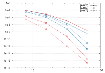
Figure 1. $\|\mathcal{E}(\cdot,1/2)\|_{L^{\infty}(10,\infty)}$ as a function of $N$ with Example 4.2 and Example 4.3 reported in blue and red, respectively.

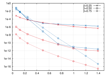
Figure 2. $\|\mathcal{E}(\cdot,t)\|_{L^{\infty}(10,\infty)}$ with $N=32$ as a function of $t$ with Example 4.2 and Example 4.3 reported in blue and red, respectively.

We consider again the two dimensional initial value problem discussed above but use the sinc quadrature approximation (4.3) with $N=40$ and $k=\ln(N)/(\beta N)$ (Example 4.2). Here we use triangle [26] to generate meshes such that each mesh is quasi-uniform and controlled by maximum area of cells. Approximation $Q_{h}^{N,k}(0.5)$ for different values of $\beta$ are provided in Figure 3, thereby illustrating the effect of $\beta$ on the diffusion strength. In addition, snapshots of $Q_{h}^{N,k}(t)$ at different times $t$ are provided in Figure 4.

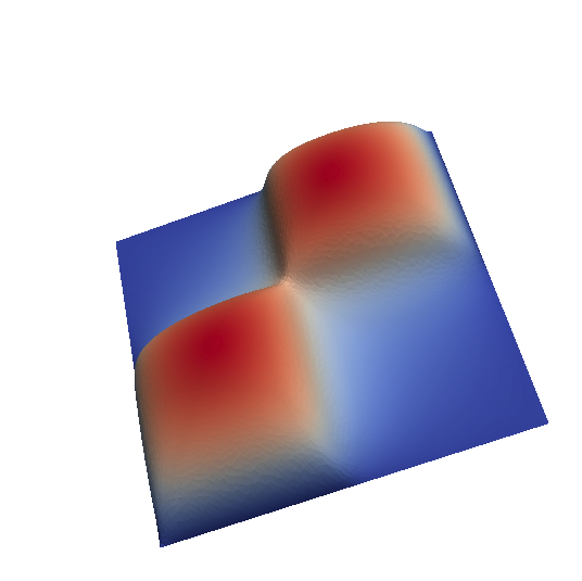
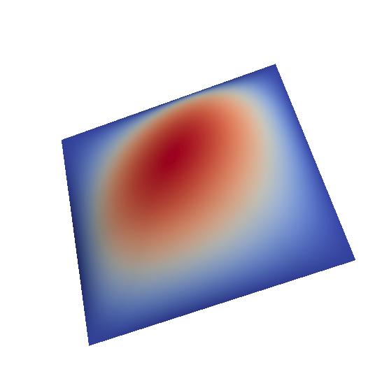
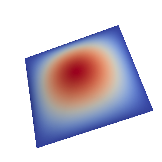
$\beta=0.25$	$\beta=0.5$	$\beta=0.75$

Figure 3. Approximations $Q_{h}^{N,k}(0.5)$ for initial data problem for different values of $\beta$. The diffusion process is faster when increasing $\beta$.

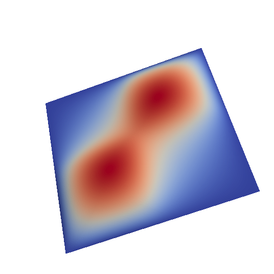
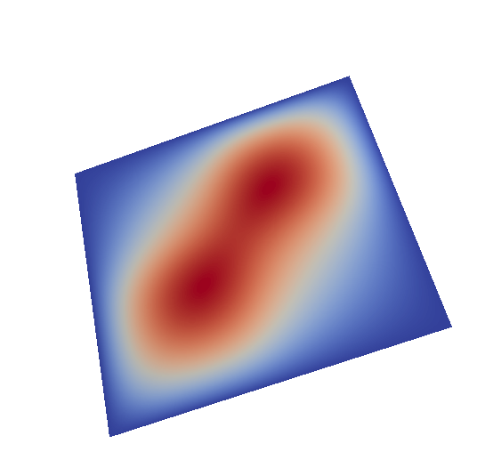
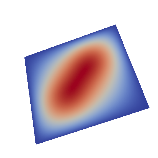
$t=1.0$	$t=1.5$	$t=2.0$

Figure 4. Evolution of the solution $Q_{h}^{N,k}(t)$ when $\beta=0.25$.

Finally, the total approximation errors, $\|Q_{h}^{N,k}(t)-u(t)\|$ at $t=0.5$, are reported in Table 5.4 for different values of $\beta$. The optimal order $2$ predicted by Corollary 4.1 is obtained for large $\beta$, while the asymptotic regime for $\beta=0.25$ was not reached in the computations.

$h^{2}$	$\beta=0.25$		$\beta=0.5$		$\beta=0.75$
$0.02$	$2.38\times 10^{-2}$		$1.47\times 10^{-3}$		$6.11\times 10^{-4}$
$0.005$	$6.20\times 10^{-3}$	$1.94$	$4.72\times 10^{-4}$	$1.64$	$1.66\times 10^{-4}$	$1.88$
$0.00125$	$1.59\times 10^{-3}$	$1.96$	$1.21\times 10^{-4}$	$1.96$	$4.32\times 10^{-5}$	$1.94$
$0.0003125$	$4.26\times 10^{-4}$	$1.90$	$3.17\times 10^{-5}$	$1.93$	$1.09\times 10^{-5}$	$1.99$
$0.000078125$	$1.13\times 10^{-4}$	$1.91$	$7.88\times 10^{-6}$	$2.01$	$2.73\times 10^{-6}$	$2.00$

Table 5.4. Total approximation error $\|Q_{h}^{N,k}(t)-u(t)\|$ at $t=0.5$ and convergence rate for initial data (5.2) with different values of $\beta$. The optimal order $2$ predicted by Corollary 4.1 is obtained for large $\beta$, while the asymptotic regime for $\beta=0.25$ was not reached in the computations.

References

• [1] O. G. Bakunin. Turbulence and diffusion: scaling versus equations, volume 101. Springer, 2008.
• [2] R. E. Bank and H. Yserentant. On the $\{$H^ 1$\}$-stability of the $\{$L_2$\}$-projection onto finite element spaces. Numerische Mathematik, 126(2):361–381, 2014.
• [3] P. W. Bates. On some nonlocal evolution equations arising in materials science. Nonlinear dynamics and evolution equations, 48:13–52, 2006.
• [4] A. Bonito and J. Pasciak. Numerical approximation of fractional powers of regularly accretive operators. IMA J Numer Anal 2016 : drw042v1-drw042.
• [5] A. Bonito and J. Pasciak. Numerical approximation of fractional powers of elliptic operators. Mathematics of Computation, 84(295):2137–2162, 2015.
• [6] J. Bramble and X. Zhang. The analysis of multigrid methods. In Handbook of numerical analysis, Vol. VII, Handb. Numer. Anal., VII, pages 173–415. North-Holland, Amsterdam, 2000.
• [7] J. H. Bramble and J. Xu. Some estimates for a weighted l2 projection. Mathematics of Computation, 56(194):463–476, 1991.
• [8] L. Caffarelli and L. Silvestre. An extension problem related to the fractional laplacian. Communications in partial differential equations, 32(8):1245–1260, 2007.
• [9] P. Constantin, A. J. Majda, and E. Tabak. Formation of strong fronts in the 2-d quasigeostrophic thermal active scalar. Nonlinearity, 7(6):1495, 1994.
• [10] P. Constantin and J. Wu. Behavior of soutions of 2d quasi-geostrophic equations. SIAM journal on the mathematical analyis, 30(5):937–948, 1999.
• [11] J. H. Cushman and T. Ginn. Nonlocal dispersion in media with continuously evolving scales of heterogeneity. Transport in Porous Media, 13(1):123–138, 1993.
• [12] E. Di Nezza, G. Palatucci, and E. Valdinoci. Hitchhiker?s guide to the fractional sobolev spaces. Bulletin des Sciences Mathématiques, 136(5):521–573, 2012.
• [13] L. C. Evans. Partial differential equations. Providence, Rhode Land: American Mathematical Society, 1998.
• [14] I. Gavrilyuk, W. Hackbusch, and B. Khoromskij. Data-sparse approximation to the operator-valued functions of elliptic operator. Mathematics of computation, 73(247):1297–1324, 2004.
• [15] I. P. Gavrilyuk, W. Hackbusch, and B. N. Khoromskij. $\mathcal{H}$-matrix approximation for the operator exponential with applications. Numerische Mathematik, 92(1):83–111, 2002.
• [16] M. Ilic, F. Liu, I. Turner, and V. Anh. Numerical approximation of a fractional-in-space diffusion equation, i. Fractional Calculus and Applied Analysis, 8(3):323–341, 2005.
• [17] M. Ilic, F. Liu, I. Turner, and V. Anh. Numerical approximation of a fractional-in-space diffusion equation (ii)–with nonhomogeneous boundary conditions. Fractional Calculus and applied analysis, 9(4):333–349, 2006.
• [18] T. Kato. Fractional powers of dissipative operators. Journal of the Mathematical Society of Japan, 13(3):246–274, 1961.
• [19] J. L. Lions and E. Magenes. Non-homogeneous boundary value problems and applications, volume 1. Springer Science & Business Media, 2012.
• [20] M. López-Fernández and C. Palencia. On the numerical inversion of the laplace transform of certain holomorphic mappings. Applied Numerical Mathematics, 51(2):289–303, 2004.
• [21] A. Lunardi. Interpolation theory. Edizioni della normale, 2009.
• [22] J. Lund and K. L. Bowers. Sinc methods for quadrature and differential equations. SIAM, 1992.
• [23] W. McLean and V. Thomee. Iterative solution of shifted positive-definite linear systems arising in a numerical method for the heat equation based on laplace transformation and quadrature. The ANZIAM Journal, 53(02):134–155, 2011.
• [24] R. H. Nochetto, E. Otarola, and A. J. Salgado. A pde approach to space-time fractional parabolic problems. SIAM Journal on Numerical Analysis 54.2 (2016): 848-873.
• [25] D. Sheen, I. Sloan, and V. Thomée. A parallel method for time-discretization of parabolic problems based on contour integral representation and quadrature. Mathematics of Computation of the American Mathematical Society, 69(229):177–195, 2000.
• [26] J. Shewchuk. Delaunay refinement algorithms for triangular mesh generation. COMPUTATIONAL GEOMETRY-THEORY AND APPLICATIONS, 22(1-3):21–74, MAY 2002. 16th Annual Symposium on Computational Geometry, HONG KONG UNIV SCI & TECHNOL, KOWLOON, PEOPLES R CHINA, JUN 12-14, 2000.
• [27] P. R. Stinga and J. L. Torrea. Extension problem and harnack’s inequality for some fractional operators. Communications in Partial Differential Equations, 35(11):2092–2122, 2010.
• [28] V. Thomée. Galerkin finite element methods for parabolic problems, volume 1054. Springer, 1984.