High Throughput combinatorial method for fast and
robust prediction of lattice thermal conductivity

Abstract

The lack of computationally inexpensive and accurate ab-initio based methodologies to predict lattice thermal conductivity, without computing the anharmonic force constants or time-consuming ab-initio molecular dynamics, is one of the obstacles preventing the accelerated discovery of new high or low thermal conductivity materials. The Slack equation is the best alternative to other more expensive methodologies but is highly dependent on two variables: the acoustic Debye temperature, $\theta_{a}$, and the Grüneisen parameter, $\gamma$. Furthermore, different definitions can be used for these two quantities depending on the model or approximation. In this article, we present a combinatorial approach to elucidate which definitions of both variables produce the best predictions of the lattice thermal conductivity, $\kappa_{l}$. A set of 42 compounds was used to test accuracy and robustness of all possible combinations. This approach is ideal for obtaining more accurate values than fast screening models based on the Debye model, while being significantly less expensive than methodologies that solve the Boltzmann transport equation.

1 Introduction

Lattice thermal conductivity, $\kappa_{l}$, plays an important role in multiple applications and technologies [1]. Thermoelectric materials [2], heat sink materials [3], rewritable density scanning-probe phase-change memories [4] or thermal medical therapies [5] are some examples in which thermal transport is the technological enabling property. During the last three decades, several theoretical models and methodologies have been developed to calculate $\kappa_{l}$ [6, 7, 8, 9, 10]. It is a trade-off: while the most quick approaches can only predict trends, accurate methods are computationally expensive and can not be implemented in high throughput (HT) frameworks, hindering the discovery of new materials with better performance [1, 11, 12]. For instance, semi-empirical models predict thermal properties at reduced computational cost but require some experimental data [6, 7, 8]. Additionally, classical molecular dynamics combined with Green-Kubo equations also produces reliable results. Although this method includes high-order scattering processes, the us of semi-empirical potentials leads to errors on the order of 50% [13, 14]. Furthermore, the extension of the Green-Kubo formalism to multiscale models has been shown to be non trivial [15]. Characterization of the anharmonic forces constants and its use in the solution of the Boltzmann transport equation, BTE, is extremely expensive which makes it unfeasible in a HT approach. Thus, for an effective prediction of $\kappa_{l}$ with HT methods, there is an advantate in approximated methods based on ab-initio characterization. i. Ab-initio is fully self-consistent and does not need experimental data or the use/generation of force fields; ii. There exists HT frameworks, such as AFLOW [16, 17, 18], that can monitor, manage, correct, and post-process the information obtained from different quantum mechanical codes.

There are three main families of approximated models based on first principles. They can be classified depending on performance, accuracy and robustness.

• The “GIBBS” quasiharmonic Debye model is the least computationally expensive approach to identify trends and simple descriptors for thermal properties, such as the Grüneisen parameters and the Debye temperature [19]. The Aflow-Gibbs-Library (AGL) framework combines this model with the Slack equation [20] based on work with noble gas crystals by Leibfried and Schlomann [21] and Julian [22] to predict $\kappa_{l}$ [23]. It reproduces correctly the ordinal ranking of the thermal conductivity for several different classes of semiconductor materials using only energy-volume curves, but suffers in comparing families with different structures.

• More accurate Grüneisen parameters can be obtained using the quasiharmonic approximation, QHA, and then used in the Slack equation [24]. However, harmonic force constants have to be calculated to build the dynamical matrix that describe the vibrational modes of the system. An alternative method proposed by Madsen et al. [24] consists of the use of lattice dynamics calculations to compute approximate relaxation scattering times at $\theta_{D}$. Both methods give $\kappa_{l}$ in reasonable quantitative agreement with experiments.

• Third order interatomic force constants (3rd IFCs) are required to calculate the phonon scattering times included in the solution of the Boltzmann transport equation, BTE [9, 10, 25]. This is the most computationally expensive method but it is the most used for highly accurate results. Once scattering processes are computed using 3rd IFCs, different schemes have been proposed to solve the BTE. The relaxation time approximation, RTA, is the simplest and predicts values on average 10% smaller than experimental quantities. The full solution requires a self-consistent iteration, but produces values very close to experiment while adding only a small computational cost compared to RTA solutions [26]. The bottle neck of both methods comes from on the computation of the 3rd order IFCs. Recently, some authors have proposed the computation of these forces using compressive sensing. However, the cost to obtain reliable results is still high [27].

Despite the different approaches developed in the last few decades, there is a lack of inexpensive, accurate, and robust methods that can be used routinely. In this article, we use different definitions of $\theta_{a}$ and $\gamma$ based on the Debye model and the QHA to obtain values for $\kappa_{l}$ using the Slack equation. Using a phenomenological approach, we compare the results obtained with our combinatorial schema to available experimental data to decide which description of these two variables best predict values for $\kappa_{l}$ with qualitative and quantitative accuracy in a high-throughput approach.

2 Methodology

2.1 Lattice thermal conductivity

The lattice thermal conductivity is computed using the Slack equation (Eq. 2.1) because of its simplicity:

$$\kappa_{l}(\theta_{a}) = \frac{0.849\times 3\sqrt[3]{(}4)}{20\pi^{3}(1-0.514\gamma^{-1}+0.228\gamma^{-2})}\times$$

$$\times\left(\frac{k_{B}\theta_{a}}{\hbar}\right)^{2}\frac{k_{B}M_{\mathrm{av}}V^{\frac{1}{3}}}{\hbar\gamma^{2}}.$$

This equation predicts $\kappa_{l}$ at the acoustic Debye temperature ($\theta_{a}$) using the Grüneisen parameter, $\gamma$, primitive cell volume, $V$, and the average atomic mass, $M_{\mathrm{av}}$. The thermal conductivity at any temperature is estimated by [20, 28, 24]:

$$\kappa_{l}(T)=\kappa_{l}(\theta_{a})\frac{\theta_{a}}{T}.$$ (2)

Equations (2.1) and (2) show that only the acoustic Debye temperature and the Grüneisen parameter are needed to calculate $\kappa_{l}$ at any temperature. Various groups have used different models to predict this quantity using the Slack equation. It seems that Slack equation combined with the Debye model tends to underestimate $\kappa_{l}$ [23], while when combined with lattice dynamics calculations, $\kappa_{l}$ is overestimated [24]. We propose the combination of both models to offset the errors and obtain values closer to the experimental results.

Our implementation is based on a combinatorial approach where the lattice thermal conductivity is a function of two variables: acoustic Debye temperature, $\theta_{a}$, and Grüneisen parameter, $\gamma$: $\kappa_{l}(\theta_{a},\gamma)$. We use different formulations based on the Debye model and quasiharmonic approximation to compute these two variables and then combine them to obtain different values for $\kappa_{l}(\theta^{x}_{a},\gamma^{y})$ (see Figure 1). We use a set of 42 materials, all belonging to different space groups and presenting a range of four orders of magnitude for $\kappa_{l}$, as a test to determine the best combination of variables from a quantitative point of view. This approach maximizes the flexibility of the method, optimizing the results without extra costs beyond the harmonic force constants calculations.

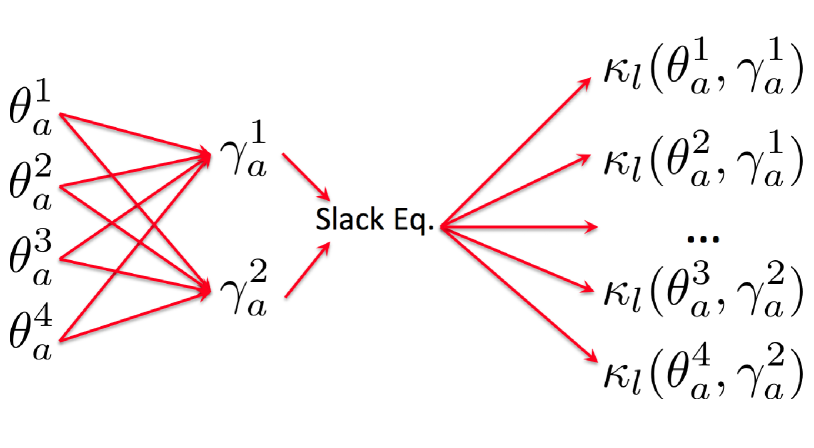
Figure 1: Combinatorial diagram for lattice thermal conductivity

The first definition for $\gamma$ is extracted from Ref. [24]:

$$\gamma^{(1)}_{a}=\sqrt{\overline{\gamma}^{2}_{a}}=\sqrt{\frac{\sum\limits_{q}\sum\limits_{i}^{\hbar\omega_{iq}<k_{B}\theta_{a}}\gamma^{2}_{iq}C_{iq}}{\sum\limits_{q}\sum\limits_{i}^{\hbar\omega_{iq}<k_{B}\theta_{a}}C_{iq}}},$$ (3)

where $\gamma_{iq}$ is defines as:

$$\gamma_{iq}=-\frac{V_{eq}^{0K}}{2\nu_{qj}^{2}}\sum_{i}e_{iq}\frac{\partial D_{q}}{\partial V}e_{iq}^{*}.$$ (4)

Since the acoustic bands provide the majority of the contribution to $\kappa_{l}$, the sum is performed over the modes, $i$, and q-points, $q$, having an energy less than $k_{B}\theta_{a}$. We propose a second definition where the sum is done only for the acoustic modes instead of over the modes having an energy less than $k_{B}\theta_{a}$:

$$\gamma^{(2)}_{a}=\sqrt{\overline{\gamma}^{2}_{a}}=\sqrt{\frac{\sum\limits_{q}\sum\limits_{i=1}^{3}\gamma^{2}_{a,iq}C_{iq}}{\sum\limits_{q}\sum\limits_{i=1}^{3}C_{iq}}}.$$ (5)

It is important to note that while $\gamma^{(1)}_{a}$ depends on $\theta_{a}$, $\gamma^{(2)}_{a}$ is independent of the other variable.

Recently, Madsen et al. also used the averaged squared Grüneisen parameters obtaining similar results with their model [29]:

$$\gamma^{(3)}=\sqrt{\overline{\gamma}^{2}}=\sqrt{\frac{\sum\limits_{q}\sum\limits_{i}\gamma^{2}_{iq}C_{iq}}{\sum\limits_{q}\sum\limits_{i}C_{iq}}}.$$ (6)

Phonon calculations can be also used to predict $\theta_{a}$:

$$\theta^{(1)}_{a}=n^{1/3}\theta_{D}=n^{1/3}\sqrt{\frac{5\hbar}{3k_{B}}\frac{\int_{0}^{\infty}\omega^{2}g(\omega)d\omega}{\int_{0}^{\infty}g(\omega)d\omega}}.$$ (7)

where $n$ is the number of atoms per unit cell and $g(\omega)$ is the phonon density of states. Similar to $\gamma^{(2)}_{a}$, we get $\theta_{a}$ using only the acoustic branches:

$$\theta^{(2)}_{a}=\sqrt{\frac{5\hbar}{3k_{B}}\frac{\int_{0}^{\infty}\omega_{a}^{2}g(\omega_{a})d\omega_{a}}{\int_{0}^{\infty}g(\omega_{a})d\omega_{a}}}.$$ (8)

The classic definition for the Debye frequency, the maximun frequency in the vibrational spectra, can be also applied to obtain the Debye temperature using the phonon density of states, pDOS:

$$\int^{\omega_{D}}_{0}g(\omega)d\omega=3n,$$ (9)

$$\theta^{(3)}_{a}=n^{1/3}\theta_{D}=n^{1/3}\frac{\hbar\omega_{D}}{k_{B}}.$$ (10)

The Debye model also predicts $\theta_{D}$ using the bulk modulus, $B$ [19, 30, 31]:

$$\theta^{(4)}_{a}=n^{1/3}\theta_{D}=n^{1/3}\frac{\hbar}{k_{B}}[6\pi^{2}V^{1/2}n]^{1/3}f(\sigma)\sqrt{\frac{B}{M}}.$$ (11)

Here, $M$ is the mass of the unit cell, and $f(\sigma)$ is given by

$$f(\sigma)=\left\{3\left[2\left(\frac{2}{3}\cdot\frac{1+\sigma}{1-2\sigma}\right)^{3/2}+\left(\frac{1}{3}\cdot\frac{1+\sigma}{1-\sigma}\right)^{3/2}\right]^{-1}\right\}^{\frac{1}{3}},$$ (12)

within the assumption that the Poisson ratio, $\sigma$, remains constant. For the calculations described in this article, this value is set at 0.25, which is the theoretical value for a Cauchy solid [19, 31]. The Poisson ratio $\sigma$ for crystalline materials is typically in the range 0.2-0.3. Bulk modulus, $B$, is obtained fitting free energy, $F(V,T)$, obtained using the QHA to the Birch-Murnaghan (BM) function:

$$F(V)=F_{eq}+\frac{BV_{eq}}{B_{p}}\Bigg{[}\frac{(V_{eq}/V)^{B_{p}}}{Bp-1}+1\Bigg{]}-\frac{V_{eq}B}{Bp-1},$$ (13)

where, equilibrium free energy, $F_{eq}$, bulk modulus, $B$, equilibrium volume, $V_{eq}$ and the derivative of the bulk modulus with respect to pressure, $B_{p}$ are used as the fitting parameters.

2.2 Computational details

Geometry optimization

All structures are fully relaxed using the automated framework, AFLOW [16, 17, 18], and the DFT Vienna Ab-initio simulation package, VASP [32]. Optimizations are performed following the AFLOW standards [18]. We use the projector augmented wave (PAW) pseudopotentials [33] and the exchange and correlation functionals parametrized by the generalized gradient approximation proposed by Perdew-Burke-Ernzerhof (PBE) [34]. All calculations use a high energy-cutoff, which is 40$\%$ larger than the maximum recommended cutoff among all component potentials, and a k-points mesh of 8,000 k-points per reciprocal atom. Primitive cells are fully relaxed (lattice parameters and ionic positions) until the energy difference between two consecutive ionic steps is smaller than $10^{-4}$ eV and forces in each atom are below $10^{-3}$ eV/Å.

2.2.1 Phonon calculations

Phonon calculations were carried out using the automatic phonon library, APL, as implemented in the AFLOW package, using VASP to obtain the IFCs via the finite-displacement approach [35]. The magnitude of this displacement is 0.015 Å. Electronic self consistent field (SCF) for single point calculations were stopped when the difference of energy between last two step was less than $10^{-8}$ eV. This threshold ensures a good convergence for the wavefunction and accurate enough values for forces and harmonic force constants. Non-analytical contributions to the dynamical matrix are also included using the formulation developed by Wang et al [36]. Frequencies and other related phonon properties are calculated on a 21$\times$21$\times$21 q-mesh in the Brillouin zone, which is sufficient to converge the vibrational density of states, pDOS, and hence the values of thermodynamic properties calculated through it. The pDOS is calculated using the linear interpolation tetrahedron method available in AFLOW package. The derivative of dynamical matrix is obtained using the central difference method within a volume range of $\pm 0.03\%$.

3 Results

A data set of 42 compounds has been used to validate our approach. The list of materials includes semiconductors and insulators that belong to different structure prototypes such as diamond, zinc blende, rock salt and fluorite. To maximize the heterogeneity of the data set, materials have been selected containing as many different elements as possible from the s-, p-, and d-blocks of the periodic table.

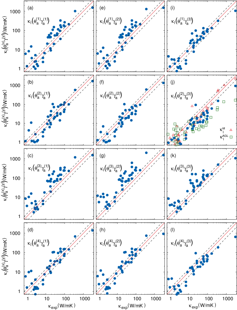
Figure 2: Lattice thermal conductivity, $\kappa_{l}(\theta_{a},\gamma)$, for the proposed models. Dashed black lines represent $\pm$40% error.

The comparison between our combinatorial approach and experimentally reported values for $\kappa_{l}$ is depicted in Figure 2. The twelve models predict qualitatively the main trend for $\kappa_{l}$. We used different statistical quantities to measure the level of qualitative and quantitative agreement between the models and the experimental data. The Pearson and Spearman correlations measure the linear correlation and the monotonicity of the relationship between the two variables respectively (see Table 1). We have found high Pearson and Spearman correlation values for some of the predicted models. For instance, $\kappa_{l}\left(\theta^{(1)}_{a},\gamma^{(3)}\right)$, $\kappa_{l}\left(\theta^{(2)}_{a},\gamma^{(3)}\right)$ and $\kappa_{l}\left(\theta^{(4)}_{a},\gamma^{(3)}\right)$ present Pearson and Spearman correlations with experiments higher than 0.90.

Table 1: Pearson and (Spearman) correlations for the material data set. Highest Pearson correlations in bold.

	$\theta^{(1)}_{a}$	$\theta^{(2)}_{a}$	$\theta^{(3)}_{a}$	$\theta^{(4)}_{a}$
$\gamma^{(1)}_{a}$	0.87 (0.88)	0.97 (0.89)	0.82 (0.90)	0.93 (0.88)
$\gamma^{(2)}_{a}$	0.80 (0.89)	0.95 (0.89)	0.64 (0.89)	0.83 (0.89)
$\gamma^{(3)}$	0.97 (0.90)	0.99 (0.90)	0.91 (0.86)	0.97 (0.90)

To test the quantitative accuracy of the different models, we also compute the root mean square relative deviation, RMSrD, for each (see Table 2). The results are far from the accuracy of the methods based on the exact solution of the BTE, however some of the combinations present interesting results considering their lower computational cost. $\kappa_{l}\left(\theta^{(2)}_{a},\gamma^{(2)}_{a}\right)$, $\kappa_{l}\left(\theta^{(2)}_{a},\gamma^{(3)}\right)$ and $\kappa_{l}\left(\theta^{(4)}_{a},\gamma^{(3)}\right)$ present a RMSrD lower than 100%. Moreover, in all cases, the major contribution to this deviation corresponds to the materials with a lower $\kappa_{l}$ in which, a small absolute error could be transform in a big relative error.

Table 2: Root mean square relative deviation (RMSrD) for the material data set. Lowest RMSrD in bold.

	$\theta^{(1)}_{a}$	$\theta^{(2)}_{a}$	$\theta^{(3)}_{a}$	$\theta^{(4)}_{a}$
$\gamma^{(1)}_{a}$	237%	120%	355%	200%
$\gamma^{(2)}_{a}$	230%	90%	435%	200%
$\gamma^{(3)}$	112%	75%	269%	99%

Combining both statistical descriptors, we can conclude that the best results are obtained for $\kappa_{l}\left(\theta^{(2)}_{a},\gamma^{(3)}\right)$. However, these results should be compared with previous models to evaluate their performance. To the best of our knowledge, the most established and accurate model to predict $\kappa_{l}$ using only harmonic force constants has been developed by Madsen et al. [29]. They used an approximated value for the phonon scattering time using the Debye temperature and the Grüneisen parameters. This method ($\kappa^{M}_{l}$) and our combinatorial approach have the same computational cost, the calculation of the harmonic force constants. The comparison between $\kappa^{M}_{l}$ and $\kappa_{l}\left(\theta^{(2)}_{a},\gamma^{(3)}\right)$ is depicted in Figure 2 (j). Both models show similar behaviors, although, the statistical descriptors are slightly different. $\kappa_{l}\left(\theta^{(2)}_{a},\gamma^{(3)}\right)$ presents a smaller RMSrD than $\kappa^{M}_{l}$ (75% and 89% respectively) and a higher Pearson correlation (0.99 and 0.98 respectively). We can also compare $\kappa_{l}\left(\theta^{(2)}_{a},\gamma^{(3)}\right)$ with less expensive methodologies such as AGL (see Figure 2 (j)). Although $\kappa^{AGL}_{l}$ captures some of the overall trends and can be used as a fast screening method, this method underestimates $\kappa_{l}$. This underestimation can be as large as an order of magnitude which is particularly detrimental to compounds with high $\kappa_{l}$ values.

4 Conclusions

A high throughput combinatorial method for fast and robust prediction of lattice thermal conductivity is presented. Using the QHA-APL implementation [35], we can compute different definitions for the Debye temperature and the Grüneisen parameter. These values can be used in a combinatorial approach with the Slack equation to obtain different values of $\kappa_{l}(\theta_{a},\gamma)$. We use a set of 42 materials to validate our results and elucidate the best combination of parameters. Best results are obtained when $\theta^{(2)}_{a}$ is used, being the most accuarte procedure to predict the acoustic Debye temperature. $\kappa_{l}\left(\theta^{(2)}_{a},\gamma^{(3)}\right)$ is the most robust and accurate of all the combinations, obtaining qualitatively and quantitatively better results than other models in the literature with similar computational cost. The methodology presented in this paper can be extremely useful because of its quantitative predictive power and its low computational cost compared to the calculation of the anharmonic force constants.

5 Acknowledgments

We would like to acknowledge support by DOD-ONR (N00014-13-1-0635, N00014-11-1-0136, N00014-09-1-0921) and by DOE (DE-AC02- 05CH11231), specifically the BES program under Grant # EDCBEE. The AFLOW consortium would like to acknowledge the Duke University - Center for Materials Genomics and the CRAY corporation for computational support.

References

- Curtarolo et al. [2013] S. Curtarolo, G. L. W. Hart, M. Buongiorno Nardelli, N. Mingo, S. Sanvito, O. Levy, The high-throughput highway to computational materials design, Nat. Mater. 12 (2013) 191–201, doi:10.1038/nmat3568.
- Zebarjadi et al. [2012] M. Zebarjadi, K. Esfarjani, M. S. Dresselhaus, Z. F. Ren, G. Chen, Perspectives on thermoelectrics: from fundamentals to device applications, Energ. Environ. Sci. 5 (2012) 5147–5162, doi:10.1039/C1EE02497C.
- Yeh and Chu [2002] L.-T. Yeh, R. C. Chu, Thermal Management of Microloectronic Equipment: Heat Transfer Theory, Analysis Methods, and Design Practices, ASME Press, 2002.
- Wright et al. [2011] C. D. Wright, L. Wang, P. Shah, M. M. Aziz, E. Varesi, R. Bez, M. Moroni, F. Cazzaniga, The design of rewritable ultrahigh density scanning-probe phase-change memories, IEEE Trans. Nanotechnol. 10 (5608505) (2011) 900–912, doi:10.1109/TNANO.2010.2089638.
- Cahill et al. [2014] D. G. Cahill, P. V. Braun, G. Chen, D. R. Clarke, S. Fan, K. E. Goodson, P. Keblinski, W. P. King, G. D. Mahan, A. Majumdar, H. J. Maris, S. R. Phillpot, E. Pop, L. Shi, Nanoscale thermal transport. II. 2003-2012, Apr. 1 (2014) 011305, doi:%****␣manuscript.tex␣Line␣500␣****http://dx.doi.org/10.1063/1.4832615.
- Ziman [1960] J. Ziman, Electrons and phonons: The theory of transport phenomena in solids., Clarendon, 1960.
- Callaway [1959] J. Callaway, Model for Lattice Thermal Conductivity at Low Temperatures, Phys. Rev. 113 (1959) 1046–1051, doi:10.1103/PhysRev.113.1046.
- Allen [1994] P. B. Allen, Zero-point and isotope shifts: Relation to thermal shifts, Phil. Mag. B 70 (3) (1994) 527–534, doi:10.1080/01418639408240227.
- Broido et al. [2007] D. A. Broido, M. Malorny, G. Birner, N. Mingo, D. A. Stewart, Intrinsic lattice thermal conductivity of semiconductors from first principles, Appl. Phys. Lett. 91 (2007) 231922.
- Wang et al. [2011] Z. Wang, S. Wang, S. Obukhov, N. Vast, J. Sjakste, V. Tyuterev, N. Mingo, Thermoelectric transport properties of silicon: Towards an ab initio approach, Phys. Rev. B 83 (2011) 205208.
- Carrete et al. [2014a] J. Carrete, W. Li, N. Mingo, S. Wang, S. Curtarolo, Finding Unprecedentedly Low-Thermal-Conductivity Half-Heusler Semiconductors via High-Throughput Materials Modeling, Phys. Rev. X 4 (2014a) 011019, doi:10.1103/PhysRevX.4.011019.
- Carrete et al. [2014b] J. Carrete, N. Mingo, S. Wang, S. Curtarolo, Nanograined Half-Heusler Semiconductors as Advanced Thermoelectrics: An Ab Initio High-Throughput Statistical Study, Adv. Func. Mater. 24 (2014b) 7427–7432, doi:10.1002/adfm.201401201.
- Green [1954] M. S. Green, Markoff random processes and the statistical mechanics of time-dependent phenomena. II. Irreversible processes in fluids, J. Chem. Phys. 22 (3) (1954) 398–413, doi:10.1063/1.1740082.
- Kubo [1957] R. Kubo, Statistical-mechanical theory of irreversible processes. I. General theory and simple applications to magnetic and conduction problems, J. Phys. Soc. Jpn. 12 (6) (1957) 570–586, doi:10.1143/JPSJ.12.570.
- Curtarolo and Ceder [2002] S. Curtarolo, G. Ceder, Dynamics of an Inhomogeneously Coarse Grained Multiscale System, Phys. Rev. Lett. 88 (2002) 255504, doi:10.1103/PhysRevLett.88.255504.
- S. Curtarolo, W. Setyawan, G. L. W. Hart, M. Jahnátek, R. V. Chepulskii, R. H. Taylor, S. Wang, J. Xue, K. Yang, O. Levy, M. J. Mehl, H. T. Stokes, D. O. Demchenko, and D. Morgan [2012] S. Curtarolo, W. Setyawan, G. L. W. Hart, M. Jahnátek, R. V. Chepulskii, R. H. Taylor, S. Wang, J. Xue, K. Yang, O. Levy, M. J. Mehl, H. T. Stokes, D. O. Demchenko, and D. Morgan, AFLOW: an automatic framework for high-throughput materials discovery, Comp. Mat. Sci. 58 (2012) 218–226, doi:10.1016/j.commatsci.2012.02.005.
- Curtarolo et al. [2012] S. Curtarolo, W. Setyawan, S. Wang, J. Xue, K. Yang, R. H. Taylor, L. J. Nelson, G. L. W. Hart, S. Sanvito, M. Buongiorno Nardelli, N. Mingo, O. Levy, AFLOWLIB.ORG: A distributed materials properties repository from high-throughput ab initio calculations, Comp. Mat. Sci. 58 (2012) 227–235, doi:10.1016/j.commatsci.2012.02.002.
- Calderon et al. [2015a] C. E. Calderon, J. J. Plata, C. Toher, C. Oses, O. Levy, M. Fornari, A. Natan, M. J. Mehl, G. L. W. Hart, M. Buongiorno Nardelli, S. Curtarolo, The AFLOW Standard for High-Throughput Materials Science Calculations, in: [37] (2015a) 233–238, doi:10.1016/j.commatsci.2015.07.019.
- Blanco et al. [2004] M. A. Blanco, E. Francisco, V. Luaña, GIBBS: isothermal-isobaric thermodynamics of solids from energy curves using a quasi-harmonic Debye model, Comput. Phys. Commun. 158 (1) (2004) 57–72, doi:10.1016/j.comphy.2003.12.001.
- Slack [1979] G. A. Slack, The thermal conductivity of nonmetallic crystals, in: H. Ehrenreich, F. Seitz, D. Turnbull (Eds.), Solid State Physics, vol. 34, Academic, New York, 1, 1979.
- Leibfried and Schlomann [1954] G. Leibfried, E. Schlomann, Warmleitund in elektrische isolierenden Kristallen, Nach. Akad. Wiss. Gottingen, Math. Phyz. Klasse 4 (1954) 71.
- Julian [1965] C. L. Julian, Theory of Heat Conduction in Rare-Gas Crystals, Phys. Rev. 137 (1965) A128–A137, doi:10.1103/PhysRev.137.A128.
- Toher et al. [2014] C. Toher, J. J. Plata, O. Levy, M. de Jong, M. D. Asta, M. Buongiorno Nardelli, S. Curtarolo, High-Throughput Computational Screening of thermal conductivity, Debye temperature and Grüneisen parameter using a quasi-harmonic Debye Model, Phys. Rev. B 90 (2014) 174107, doi:10.1103/PhysRevB.90.174107.
- Bjerg et al. [2014] L. Bjerg, B. B. Iversen, G. K. H. Madsen, Modeling the thermal conductivities of the zinc antimonides ZnSb and Zn4Sb3, Phys. Rev. B 89 (024304) (2014) 0243041–0243048, doi:10.1103/PhysRevB.89.024304.
- Deinzer et al. [2003] G. Deinzer, G. Birner, D. Strauch, Ab initio calculation of the linewidth of various phonon modes in germanium and silicon, Phys. Rev. B 67 (144304) (2003) 1443041–1443046, doi:%****␣manuscript.tex␣Line␣675␣****10.1103/PhysRevB.67.144304.
- Shindé and Srivastava [2014] S. L. Shindé, G. P. Srivastava (Eds.), Ab Initio Thermal Transport, Springer, 137–173, 2014.
- Zhou et al. [2014] F. Zhou, W. Nielson, Y. Xia, V. Ozoliņš, Lattice Anharmonicity and Thermal Conductivity from Compressive Sensing of First-Principles Calculations, Phys. Rev. Lett. 113 (2014) 185501, doi:10.1103/PhysRevLett.113.185501.
- Morelli and Slack [2006] D. T. Morelli, G. A. Slack, High Lattice Thermal Conductivity Solids, in: S. L. Shindé, J. S. Goela (Eds.), High Thermal Conductivity Materials, Springer, 2006.
- Madsen et al. [2016] G. K. H. Madsen, A. Katre, C. Bera, Calculating the thermal conductivity of the silicon clathrates using the quasi-harmonic approximation, Phys. Stat. Solidi A 213 (2016) 802–807, doi:10.1002/pssa.201532615.
- Blanco et al. [1996] M. A. Blanco, A. M. Pendás, E. Francisco, J. M. Recio, R. Franco, Thermodynamical properties of solids from microscopic theory: Applications to MgF2 and Al2O3, J. Mol. Struct., Theochem 368 (1-3 SPEC. ISS.) (1996) 245–255, doi:10.1016/S0166-1280(96)90571-0.
- Poirier [2000] J.-P. Poirier, Introduction to the Physics of the Earth′ s Interior, Cambridge University Press, 2nd edn., 2000.
- Kresse and Hafner [1993] G. Kresse, J. Hafner, Ab initio molecular dynamics for liquid metals, Phys. Rev. B 47 (1993) 558–561.
- Blöchl [1994] P. E. Blöchl, Projector augmented-wave method, Phys. Rev. B 50 (1994) 17953–17979.
- Perdew et al. [1996] J. P. Perdew, K. Burke, M. Ernzerhof, Generalized gradient approximation made simple, Phys. Rev. Lett. 77 (1996) 3865–3868.
- Nath et al. [2016] P. Nath, J. J. Plata, D. Usanmaz, R. Al Rahal Al Orabi, M. Fornari, M. Buongiorno Nardelli, C. Toher, S. Curtarolo, High-Throughput Prediction of Finite-Temperature Properties using the Quasi-Harmonic Approximation, arXiv:1603.06924 Submitted.
- Wang et al. [2010] Y. Wang, J. J. Wang, W. Y. Wang, Z. G. Mei, S. L. Shang, L. Q. Chen, Z. K. Liu, A mixed-space approach to first-principles calculations of phonon frequencies for polar materials, J. Phys.: Condens. Matter 22 (20) (2010) 202201, doi:10.1088/0953-8984/22/20/202201.
- Calderon et al. [2015b] C. E. Calderon, J. J. Plata, C. Toher, C. Oses, O. Levy, M. Fornari, A. Natan, M. J. Mehl, G. L. W. Hart, M. Buongiorno Nardelli, S. Curtarolo, The AFLOW Standard for High-Throughput Materials Science Calculations, Comp. Mat. Sci. 108 Part A (2015b) 233–238, doi:10.1016/j.commatsci.2015.07.019.