Natural Steganography:
cover-source switching for better steganography

Abstract

This paper proposes a new steganographic scheme relying on the principle of “cover-source switching”, the key idea being that the embedding should switch from one cover-source to another. The proposed implementation, called Natural Steganography, considers the sensor noise naturally present in the raw images and uses the principle that, by the addition of a specific noise the steganographic embedding tries to mimic a change of ISO sensitivity. The embedding methodology consists in 1) perturbing the image in the raw domain, 2) modeling the perturbation in the processed domain, 3) embedding the payload in the processed domain. We show that this methodology is easily tractable whenever the processes are known and enables to embed large and undetectable payloads. We also show that already used heuristics such as synchronization of embedding changes or detectability after rescaling can be respectively explained by operations such as color demosaicing and down-scaling kernels.

I Introduction

Image steganography consists in embedding a undetectable message into a cover image to generate a stego image, the application being the transmission of sensitive information. As Cachin proposed in [1], one theoretical approach proposed for steganography is to minimize a statistical distortion, and the author proposes to use the Kullback-Leibler divergence. It is interesting to note that this line of research has been rarely used as a steganographic guideline with few notable exceptions such as model-based steganography [2] which mimics the Laplacian distributions of DCT coefficients during the embedding, HUGO [3] whose model-correction mode tries to minimize the difference between the model of the cover image and the stego image, and more recently the mi-pod steganographic scheme [4] which minimizes a statistical distortion (a deflexion coefficient) between normal distributions of cover and stego contents.

Currently the large majority of steganographic algorithms are based on the use of a distortion (also called a cost) which is computed for each pixel, and which is combined with a coding scheme that minimizes the global distortion while embedding a given payload. Classical distortions functions such as the ones proposed by S-UNIWARD [5] or by HILL [6] try to infer the detectability of each pixel by assigning small costs to pixels that are difficult to predict (usually textural parts of the image) and by assigning large costs to pixels that are easy to predict (belonging to homogeneous areas and to some extend to edges). Note that a recent trend of research [7, 8] proposes to correlate embedding changes on neighboring pixels by adjusting the cost w.r.t the history of the embeddings performed on disjoint lattices in order to decrease the detectability on greyscale images or on color images [9].

Once the distortion is computed, a steganographic scheme can either simulate the embedding by sampling according to the modifications probabilities $\pi_{k},$ $k\in[1,\dots,Q]$ for a Q-arry embedding, or can directly embed the message using Syndrome Trellis Codes (STCs) [10] or multilayer STCs [10, 11]. The size of the embedding payload $N$ is computed as $N=\sum\pi_{k}\log\pi_{k}$ for each pixel of the image, and in practice the STCs succeed to reach 90% to 95% of the capacity [10] and consequently are close to optimal.

Another ingredient to tend to undetectable steganography is to use the information contained in a “pre-cover”, i.e. the high resolution image that is used to generate the cover at a lower resolution, in order to weight the cost w.r.t the rounding error. For quantization or interpolation operations, a pixel of the pre-cover at equal distance between two quantization cells will have a lower cost than a pre-cover pixel very close to one given quantization cell. This strategy has been used in Perturbed-Quantization [12] but also adapted in more recent schemes using side information [13].

The proposed paper uses similar ingredients shared by modern steganographic methods, namely model-based steganography, Q-arry embedding and the associated modification probabilities $\pi_{k}$, and side-information. The main originality of this paper relies on the possible definitions of cover sources and the use of cover-source switching to generate stego contents whose statistical distributions are very close to cover contents.

I-A What’s a source?

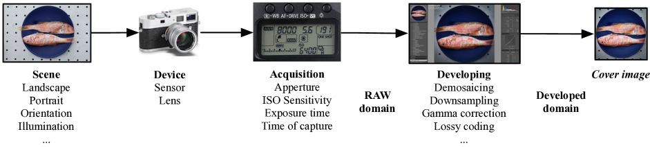
Figure 1: Pipeline of the cover image generation process which can be decomposed into four main steps (scene, device, acquisition, developing) representing parameters of whole process.

If the term “source” has been first coined with the problem of “cover-source mismatch” after the BOSS contest [14, 15] in order to denote poor steganalysis performances whenever a steganalyzer was trained with an image database coming from a set of “sources” and tested on another set. In this case the term “source” was associated with a camera device, and other authors [16] have associated a “source” with a “user” that would upload a set of pictures on a sharing platform such as FlickR.

We argue here that a source can be defined w.r.t. the image generation process depicted in Figure 1 which shows that the creation of a cover image is linked to the intervention of different parameters represented by (1) the scene that is captured, (2) the device which is used, (3) the acquisition settings used during the capture and (4) the developing step.

Each parameter is linked with a set of sub-parameters. The scene fluctuates according to the subject, but also according to the illumination or the orientation of the camera. The device is composed mainly of two elements: the sensor (which can be CMOS, CDD, color or monochrome) and the lens. The acquisition phase relies on three parameters originating from the device: the lens aperture, the ISO sensitivity and the exposure time and one parameters which is the time of capture. The developing step contains lot of processing steps such as gamma correction, demosaicing, downsampling, JPEG compression, … it can be done directly within the camera or using a developing software such as the open-source dcraw software [17] or the commercial Lightroom$\copyright$ software.

Within this paradigm, the classical usage of the term “source” as referred in [14, 15, 16] represents a setup where the device or more exactly the sensor, is constant, but a source can also reflect a situation where only a subset of parameters is constant, such as for example demosaicing algorithm, the ISO setting, the aperture… Note that in the first case the variations between images produced from the same source will be extremely large, even if as shown in [16] it will be possible to separate one source from another, however in the second scenario the variation between images can be very subtle if only one parameter, such as for example the time of capture, changes for a given source. Practically all possible sources are realistic: a casual photographer using a smartphone will usually adopt ’auto’ mode where the acquisition parameters and the developing step can fluctuate a lot, and a professional photograph will tend to choose manually his acquisition parameters (in order for example to minimize the ISO setting) and its developing process.

I-B Steganography via cover-source switching

The key idea of this paper is to propose a steganographic scheme where the message embedding will be equivalent to switching from one source $\mathcal{S}_{1}$ to another source $\mathcal{S}_{2}$; this practically can be done by designing an embedding that, when applied on $\mathcal{S}_{1}$, mimics the statistical properties of $\mathcal{S}_{2}$. More specifically in this paper we have decided to use the sensor noise to model a given source because its statistical model is rather simple, and to perform the embedding in such a way that the statistical properties of the stego images mimic the sensor noise of source $\mathcal{S}_{2}$. If we refer to Figure 1, it means that the only parameters which is fluctuating for this source is the time of capture. As we shall see in sections II, III and IV, the difference between $\mathcal{S}_{1}$ and $\mathcal{S}_{2}$ will stem in the ISO sensitivity. One can argue that this parameter is reported in the EXIF file of the image, but EXIF information can be easily edited or even removed using software such as exiftool [18].

Note that this idea of steganography based on mimicking sensor noise is far from being new. In 1999 Franz and Pfitzmann [19] propose a paradigm for a stego-system “simulating a usual process of data processing” where the usual process is defined by the scan process, in this paper the authors study the properties of scanning noise coming from different scanners. A practical implementation of this concept in proposed in 2005 by Franz and Schneidewind [20], where the authors model the sensor noise for each pixel by a Normal distribution and perform the embedding by first estimating the noiseless scan and secondly adding a noise mimicking the sensor noise. The algorithm was benchmarked using features derived from wavelet higher order statistics [21] and showed relatively good performance compared with naive noise addition. It is important to notice that contrary to the work presented here, if the idea of mimicking the sensor noise is present in [21], it doesn’t rely on neither cover-source switching nor a sharp physical model of the noise in the RAW domain.

Another requirement in order to achieve practical embedding is to be able to compute the probability of embedding changes $\pi_{k}$ in the developed domain, this in order to perform the practical embedding but also in order to compute the embedding rate. This particular aspect will be addressed in sections III and IV. Because the embedding scheme relies on the natural statistical noise of the sensor, we decided to call this steganographic scheme “Natural Steganography” (NS).

The paper is organized as follows: the next section presents the method which is used to estimate the camera sensor noise of one given cover-source from raw images, section III explains how to compute the noise mimicking another cover-source in the RAW domain. When in the developed domain the developing step is basic, the related embedded payload is also computed. Section IV describes the embedding when the developing step is more elaborated, three examples are analyzed the gamma correction operation and image downsampling. Evolutions of the embedded payload w.r.t these operations are also provided. Finally section V describes the building of a new image database coming from a monochrome sensor and presents the detectability results related to Natural Steganography. These results are compared to two state of the art algorithms which are S-Uniward and S-Uniward using side-information coming from the conversion from 16-bit to 8-bit. The detectability after gamma correction or different downsampling schemes is also provided.

I-C Notations

- Capital letters will denote random variables, bold letter denote vectors or matrices whenever explicitly mentioned.

- Indexes $(i,j)$ will usually denotes the location of the photo-site or the pixel in a given image, and the index $k$ denotes a modification $+k$ on the cover image. Note that these indexes will be omitted if not necessary for the formula.

- Notation $\bar{a}$ denotes the version of $a$ after the developing step. Each element of respectively the raw cover and the raw stego are denoted $x_{i,j}$ and $y_{i,j}$ and each element of the developed cover and the developed stego are then denoted $\bar{x}_{i,j}$ and $\bar{y}_{i,j}$ . The sensor noise is denoted $n_{i,j}$, and the stego signals in the raw domain and in the developed domain are respectively denoted $s_{i,j}$ and $\bar{s}_{i,j}$. The virtual noiseless raw signal is denoted $\mathrm{E}[S_{i,j}]=\mu$. The probability of adding $k$ on pixel or photo-site $\bar{s}_{i,j}$ is denoted $\pi_{i,j,k}=\mathrm{Pr}[\bar{S}_{i,j}=k]$.

- The 2D convolution between a matrix $\mathbf{m}$ and a filter $\mathbf{f}$ is denoted $\mathbf{m}\star\mathbf{f}$.

II Sensor noise estimation and developing pipeline

We present in this section the different noises affecting the sensor during a capture and then explain how to estimate the sensor noise. The last subsection summarizes the image developing pipeline.

II-A Sensor noise model

Camera sensor noise models have been extensively studied in numerous publications [22, 23, 24] and have already been used in image forensics for camera device identification [25, 26]. These models can only be applied to linear sensors such as CDD or CMOS sensors, but this encompass the majority of modern digital cameras at the date the paper is written. A camera sensor is decomposed into a 2D array of photo-sites and the role of each photo-site is to convert $k_{p}$ photons hitting its surface during the exposure time into a digit. The conversion involves the quantum efficiency of the sensor measuring the ratio between $k_{p}$ and the number of charge units $k_{e}$ accumulated by the photo-site during the exposure time. $k_{e}$ is then converted into a voltage, which is amplified by a gain $K$ (where $K$ is referred as the system overall gain [24]) and then quantized.

For each photo-site at location $(i,j)$, the converted signal $x(i,j)$ originates from two components:

• The “dark” signal $x_{d}(i,j)$ with expectation $\mathrm{E}[X_{d}(i,j)]=\mu_{d}$ which accounts for the number of electrons present without light and depends on the exposure time and ambient temperature,

• The “electronic” signal $x_{e}(i,j)$ with expectation $\mathrm{E}[X_{e}(i,j)]=K\mu_{e}$, which accounts for the number of electrons originating from photons coming from the scene which is captured.

The expectation $\mu$ of each photo-site response is equal to:

$$\mu_{i,j}=\mathrm{E}[X(i,j)]=\mathrm{E}[X_{d}(i,j)]+\mathrm{E}[X_{e}(i,j)]=\mu_{d}+K\mu_{e}.$$ (1)

Beside the signal components, there are three types of noise affecting the acquisition:

1. The “shot noise” associated with the electronic signal with accounts for the fluctuation of the number of charge units. Because the electronic signal comes from the variation of counting events, it has a Poisson distribution $X_{e}(i,j)\sim\mathcal{P}(\mu_{e})$ and can be approximated in a continuous setting by a normal distribution $\mathcal{N}(\mu_{e},\sigma_{e}^{2})$ with $\sigma_{e}^{2}=\mu_{e}$, hence the noise associated to the electronic signal is distributed as $\mathcal{N}(0,\mu_{e})$. Additionally this noise is independently distributed for each photo-site. An illustration of the sensor noise is provided in Figure 2.

2. The noise related to the “read-out” and the amplifier circuit. The read-out noise associated to the dark signal is independant and normally distributed as $\mathcal{N}(0,\sigma_{d}^{2})$ and it is constant for a given camera.

3. The quantization noise, which is independant and uniformly distributed with variance $\sigma_{q}^{2}=\Delta^{2}/12$ where $\Delta$ denotes the quantization step.

Since these noises are mutually independent, the variance of the sensor noise can then be expressed as [24]:

$$\sigma_{s}^{2}=K^{2}\sigma_{d}^{2}+\sigma_{q}^{2}+K(\mu-\mu_{d}).$$ (2)

In the sequel, we make the following approximations for a given cover-source: we assume that the system gain $K$ is constant for a given $ISO$ setting, that the dark signal is constant with negligible variance ($\sigma_{d}^{2}=0,\mu_{d}=\mathrm{cte_{2}})$, and that the quantization noise is negligible w.r.t. the shot noise ($\sigma_{q}^{2}=0$). As we shall see in V-D the two first assumptions have negligible impact on the performance of the scheme and that the last assumption does not impact the performance of the steganographic system whenever 16-bit quantization is considered as side-information. Finally we also assume that the spacial non-uniformity of the sensor, which is associated with the photo response non-uniformity (PRNU) and the dark signal non-uniformity (DSNU), is negligible.

For a given ISO setting $ISO_{1}$, the global sensor noise $N_{i,j}^{(1)}$ can be approximated using Eq. (2) and the above-mentioned assumptions as normally and independently distributed. We have consequently a linear relation between the sensor noise variance and the photo-site expectation $\mu$:

$$N_{i,j}^{(1)}\sim\mathcal{N}(0,a_{1}\mu_{i,j}+b_{1}).$$ (3)

The acquired photo-site sample $x_{i,j}^{(1)}$ is given by:

$$x_{i,j}^{(1)}=\mu_{i,j}+n_{i,j}^{(1)},$$ (4)

and $X\sim\mathcal{N}(\mu,a_{1}\mu_{i,j}+b_{1})$.

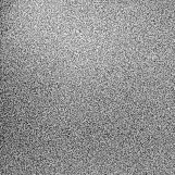
Figure 2: Illustration of the sensor noise $n$ on a picture at 2000 ISO captured with the Leica Monochrome camera. Inactivate the interpolation process of your pdf viewer for correct rendering. The pixel amplitudes are scaled for vizualisation purposes.

II-B Sensor noise estimation

In order to estimate the model of the sensor noise (i.e. the couple of parameters $(a,b)$) for a given camera model and a given ISO setting, we adopt a similar protocol as the one proposed in [23].

We first capture a set of $N_{a}$ raw images of a printed photo picturing a rectangular gradian going from full black to white. The camera is mounted on a tripod and the light is controlled using a led lightning system in a dark room. The raw images are then converted to PPM format (for color sensor) or to PGM format (for B&W sensor) using the dcraw open-source software [17] using the command:

dcraw -k 0 -4 file_name

which signify that the dark signal is not automatically removed (option -k =0), and that the captured photo-sites are not post-processed and plainly converted to 16-bit (option -4).

In order to have a process independant of the quantization, the photo-site outputs are first normalized by dividing them by $y_{max}=2^{16}-1$. The range of possible outputs is divided into $1/\delta$ segments of width $\delta$. Each normalized photo-site location is assigned to one subset of photo-sites $\mathcal{S}_{\ell}$ according to its empirical expectation over the acquired images $\hat{\eta}_{i,j}=\left(\sum_{l=1}^{N_{a}}y_{i,j}^{(l)}/y_{max}\right)/N_{a}$. The subset index is $\text{$\ell$}=\left[\hat{\eta}_{i,j}/\delta\right]$ where $\left[.\right]$ denotes the integer rounding operation. Once the segmentation into subsets is performed, the empirical mean is:

$$\hat{\mu}_{\ell}=\frac{1}{|S_{\ell}|}\sum_{i=1}^{|S_{\ell}|}\mathcal{S}_{\ell}(i),$$ (5)

where $\mathcal{S}_{\ell}(i)$ denotes the value of a photo-site belonging to the subset $\mathcal{S}_{\ell}$ and $|.|$ denotes the cardinal of a set.

The unbiased variance associated to each subset as:

$$\hat{\sigma}_{\ell}^{2}=\frac{1}{|S_{\ell}|-1}\sum_{i=1}^{|S(\ell)|}\left(\mathcal{S}_{\ell}(i)-\hat{\mu}_{\ell}\right)^{2}.$$ (6)

As an illustration, Figure (3) plots the relation in solid lines between $\hat{\mu}_{\ell}$ and $\hat{\sigma}_{\ell}^{2}$ for $N_{a}=20$ raw images captured with a Leica M Monochrome Type 230 at 1000 ISO and 1250 ISO for $\delta=5\,10^{-5}$.

The last step consists in estimating the parameters $(\hat{a},\hat{b})$, this is done by linear regression $\tilde{\sigma}_{N}^{2}=f(\hat{\mu})=\hat{a}\hat{\mu}+\hat{b}$. We see on the same figure that the linear relation, depicted by the dashed lines, is rather accurate.

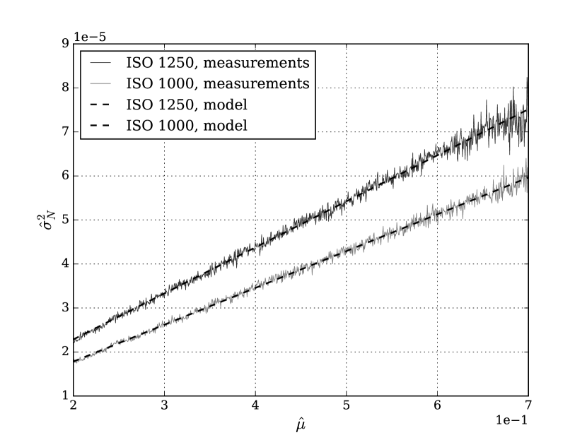
Figure 3: Sensor noise estimation for the Leica Monochrome camera and 1000 IS0 and 1250 ISO on normalized images. The estimated coefficients of the linear model are respectively $(a_{1},b_{1})=(8.36\,10^{-5},1.11\,10^{-6})$ and $(a_{2},b_{2})=(10.46\,10^{-5},1.95\,10^{-6})$ for this setup.

II-C The developing pipeline

Figure 4: The image developing pipeline.

Since the goal of any steganographic scheme is to embed message on a published image and not a raw one, we recall briefly in this subsection the different steps leading to the generation of a developed picture. The image developing pipeline, depicted on Figure 4 will be further used in sections III and IV.

In a raw image each photo-site is usually represented using 12 or 14 bits per channel depending on the sensor bit depth, and most of the color digital cameras only record one color component per photo-site. Depending of the computational power the following process can be performed either using either double, float or unsigned integer 16-bit precision.

The first step consist in interpolating for each photo-site the two missing color components via the demosaicing process (see also section sub:Demosaicing-and-color). This process can be linear or non-linear.

A color transform is then applied, and converts the original camera color domain to the reference domain XYZ (this transform depends on the camera make) and then to a color space such as sRGB, adobe RGB, wide RGB, … The white balance correction can also performed at this stage. All the color conversion operations can be expressed as multiplications by $3\times 3$ matrices and are consequently linear.

The color components are then corrected using the classical gamma correction $y=x^{1/\gamma}$ which is a non-linear sample-wise transform.

The next step encompasses a large set of possible processing operations and consists in processing the image by applying for example local contrast enhancement, denoising, adding grain, changing the contrast, … and applying geometrical transforms such as cropping, image rescaling (up-sampling or down-sampling), rotation, lens-distortion compensation, …

The last step of this pipeline consists in exporting the image in a lossy compressed format such as JPEG or a lossless format such as PNG, in each case a quantization to 8-bit/channel is performed.

Note that depending on developing software which is used, this pipeline can be completely known whenever the software source code is public, or unknown if the software is private, but this does not mean for the last case that the processing operation cannot be reverse-engineered.

III Embedding for OOC monochrome pictures

We first propose in this section a steganographic system practically working for a basic developing setup, this system is realistic for a monochrome sensor where nor demosaicing neither color transform is possible. As depicted in Figure 5, we also assume that the developed images do not undergo gamma correction or further processing and only suffer 8-bit quantization. We can call this type of images “Out Of Camera” (OOC) Pictures. In the next section we show how to deal with more advanced developing processes.

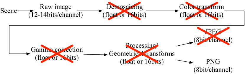
Figure 5: The basic developing pipeline associated to a monochrome sensor.

III-A Principle of the embedding

We propose to model the stego signal $S_{i,j}$ is such a way that it mimics the model of images captured at $ISO_{2}>ISO_{1}$.

Based on the assumptions made in II-A, the equivalent of (3) and (4) for a camera sensitivity parameter $ISO_{2}$ are $N_{i,j}^{(2)}\sim\mathcal{N}(0,a_{2}\mu_{i,j}+b_{2})$ and $x_{i,j}^{(2)}=\mu_{i,j}+n_{i,j}^{(2)}$.

Since the sum of two independent noises normally distributed is normal with the variances summing up, we can write that $x_{i,j}^{(2)}=\mu_{i,j}+n_{i,j}^{(1)}+s^{\prime}_{i,j}=x_{i,j}^{(1)}+s^{\prime}_{i,j}$ with $S^{\prime}_{i,j}\sim\mathcal{N}(0,(a_{2}-a_{1})\mu_{i,j}+b_{2}-b_{1})$ representing the noise necessary to mimic image captured at $ISO_{2}$.

Assuming that the observed photo-site is very close to its practical expectation, i.e. that $\mu_{i,j}\simeq x_{i,j}^{(1)}$, $x{}_{i,j}^{(2)}$ can be approximated by:

$$x_{i,j}^{(2)}\simeq x_{i,j}^{(1)}+s{}_{i,j}\triangleq y_{i,j},$$ (7)

with:

$$S_{i,j}\sim\mathcal{N}(0,(a_{2}-a_{1})x_{i,j}^{(1)}+b_{2}-b_{1}),$$ (8)

adopting the following notations $a^{\prime}\triangleq a_{2}-a_{1}$, $b^{\prime}\triangleq b_{2}-b_{1}$ , $\sigma_{S}^{2}\triangleq a^{\prime}x_{i,j}^{(1)}+b^{\prime}$, and the photo-site of the stego image is distributed as:

$$Y_{i,j}\sim\mathcal{N}(x_{i,j}^{(1)},\sigma_{S}^{2}).$$ (9)

Note that equation (7) shows explicitly the principle of cover-source switching which is simply represented in this case by adding an independant noise on each image photo-site to generate the stego photo-site $y_{i,j}$. The distribution of the stego signal in the continuous domain (see (8)) takes into account the statistical model of the sensor noises estimated for two ISO settings using the procedure presented in section II-A.

III-B 16-bit to 8-bit quantization

For OOC images, the only developing process lies in the 8-bit quantization function, consequently the goal here is to compute the embedding changes probabilities $\pi_{i,j}(k)=\mathrm{Pr}[\bar{S}_{i,j}=k]$ after this process.

These probabilities can be either used to simulate optimal embedding, or cost additive costs $\rho_{i,j}$ can be derived and used to feed a multilayered Syndrome Trellis Code using the “flipping lemma” [10] as $\rho_{i,j}=\ln\left(\tilde{\pi}_{i,j}/(1-\tilde{\pi}_{i,j})\right)$ with $\tilde{\pi}_{i,j}=\max\left\{\pi_{i,j},1-\pi_{i,j}\right\}$ (see also section VI of [10] for Q-ary embedding and multi-layered constructions).

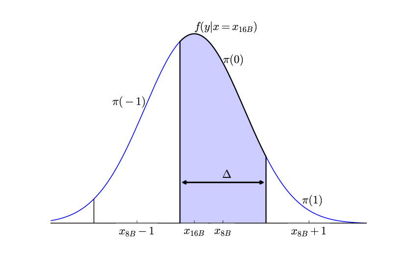
Figure 6: Computation of the embedding probabilities after 8-bit quantization.

We use the high resolution continuous assumption given by (10) and then we compute the discretized probability mass function after a quantization step of size $\Delta$ (typically $\Delta=256$ by quantizing from 16-bit resolution to 8-bit resolution).

The distribution of the stego photo-site $y$ for a given cover photo-site value coded using 16 bits $x_{16B}$ is depicted in Figure (6).

The embedding probabilities are directly linked to the 8 bits quantized value $x_{8B}=Q_{\Delta}(x_{16B})$ - where $Q_{\Delta}(.)$ denotes the quantization function - and the pdf of the Normal distribution:

$$\begin{array}[]{ccc}\pi(k)&=&\intop_{u_{k}}^{u_{k+1}}f(y|x=x_{16B})dy,\\ &=&\frac{1}{2}\left(\mathrm{erf}\left(\frac{u_{k+1}-x_{16B}}{2\sigma_{S}^{2}}\right)-\mathrm{erf}\left(\frac{u_{k}-x_{16B}}{2\sigma_{S}^{2}}\right)\right),\end{array}$$ (10)

with $u_{k}=x_{8B}-(0.5-k)\Delta$..

Once the embedding probabilities are computed for each pixel, it’s possible to derive the payload size using the entropy formula:

$$H(\overline{S})=-\sum_{i,j,k}\pi_{i,j}(k)\log_{2}\pi_{i,j}(k).$$ (11)

IV Embedding with advanced developing

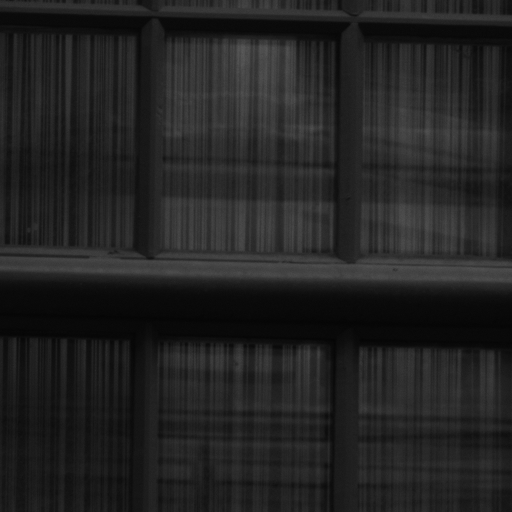
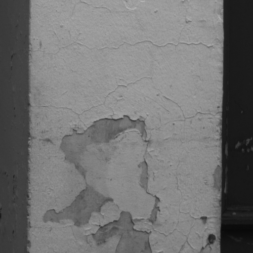
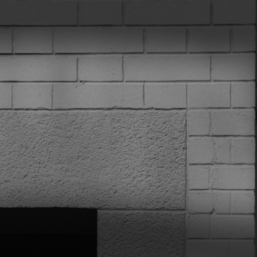
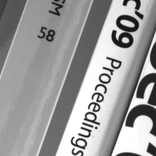
Figure 7: Six samples from MonoBase.

The main challenge of Natural Steganography is to be able to sample the stego signal in the developed domain (i.e. $\bar{S}_{i,j}$). This task can be challenging whenever the developing process is either unknown or difficult to model. On the contrary whenever the transform is non-linear but sample-wise, or linear vector-wise, the distribution of the stego signal $S$ can be computed, possibly using conditional distributions. In order to give “proof of concept implementations”, we focus here on popular processes which are (1) gamma correction, (2) demosaicing, (3) color transform and (4) down-sampling.

Note that except for the JPEG-compression which is left for further works, these processes address the main limitations of the embedding method proposed in section III.

IV-A Gamma correction

The gamma correction is a sample-wise operation defined by $y_{\gamma}\triangleq\Gamma(y)=y_{max}(y/y_{max})^{1/\gamma}$ with $y_{max}=2^{16}-1$, its inverse transform given by $\Gamma^{-1}(y)=y_{max}(y_{\gamma}/y_{max})^{\gamma}$.

In order to compute the distribution of the stego signal after gamma correction, one can simply compute the distribution of the transform of a continuous variable as:

$$\begin{array}[]{ccc}f_{Y_{\gamma}}(y_{\gamma})&=&f_{Y}(y_{\gamma})\frac{d}{dy}\Gamma^{-1}(y),\\ &=&\frac{1}{\sqrt{2\sigma_{S}^{2}\pi}}\mathrm{exp}\left(-\frac{\left(y_{\gamma}-x^{(1)}\right)^{2}}{2\sigma_{S}^{2}}\right)\gamma(y_{\gamma}/y_{max})^{\gamma-1}.\end{array}$$ (12)

However, since in practice $\sigma_{S}\ll x^{(1)}$ we can use a first order taylor expansion of the gamma correction, given by:

$$\begin{array}[]{ccc}y_{\gamma}&\simeq&\Gamma(x^{(1)})+(y-x^{(1)})(x^{(1)}/y_{max})^{1/\gamma-1}/\gamma,\\ &=&\Gamma(x^{(1)})+\alpha s,\end{array}$$ (13)

with $\alpha=(x^{(1)}/y_{max})^{1/\gamma-1}/\gamma$. This means that the gamma correction acts as an affine transform on the stego signal.

Consequently, as a first approximation, the stego signal $S_{\gamma}$ after gamma correction can be considered as normally distributed:

$$S_{\gamma}\sim\mathcal{N}(0,\alpha^{2}\sigma_{S}^{2}),$$ (14)

and the distribution of the stego photo-site is given by:

$$Y_{\gamma}\sim\mathcal{N}(z_{\gamma}(x^{(1)}),\alpha^{2}\sigma_{S}^{2}).$$ (15)

Because gamma correction is a sample-wise operation, the stego signal is independently distributed, and the embedding probabilities after 8-bit quantization can be directly computed as:

$$\begin{array}[]{ccc}\pi_{\gamma}(k)&=&\intop_{u^{\prime}_{k}}^{u^{\prime}_{k+1}}f(y_{\gamma}|x=\Gamma(x_{16B}))dy,\\ &=&\frac{1}{2}\left(\mathrm{erf}\left(\frac{u^{\prime}_{k+1}-\Gamma(x_{16B})}{2\alpha^{2}\sigma_{S}^{2}}\right)-\mathrm{erf}\left(\frac{u^{\prime}_{k}-\Gamma(x_{16B})}{2\alpha^{2}\sigma_{S}^{2}}\right)\right),\end{array}$$ (16)

with $u^{\prime}_{k}=x^{\prime}_{8B}-(0.5-k)\Delta$, $x^{\prime}_{8B}=Q_{\Delta}(\Gamma(x_{16B}))$. The payload size is consequently given as $H(\overline{S}_{\gamma})=-\sum_{i,j,k}\pi_{\gamma,i,j}(k)\log_{2}\pi_{\gamma,i,j}(k)$.

IV-B Demosaicing and color images

The goal of demosaicing is to predict for each photo-site the two missing color channels from neighboring photo-sites that, through the Color Filter Array, record other channels. Popular demosaicing schemes include bi-linear filtering which use linear interpolation from the neighbors of the same channel, or Variable Number of Gradients (VNG) [27], Patterned Pixel Grouping (PPG) [28], Adaptive Homogeneity-Directed (AHD) [29], which are more advanced schemes using the correlation between the channels to predict the one recorded by the photo-site but also edge-directionality and color homogeneity. Note that the implementation of these algorithms is available in dcraw or the library libraw [30]. One notable point of the demosaicing procedure is that the recorded photo-sites values stay unchanged and the sensor noise is still distributed as (3) for unpredicted values.

Without loss of generality we assume that there is no other operations in the developing process than demosaicing, we can consequently have a straightforward implementation of NS for color images by (1) embedding the message on the photo-site values using the algorithm proposed in section III and (2) performing the demosaicing process to generate the Stego image. The message will be then be decoded only from the non-interpolated values.

One important consequence is that the embedding ratio for a given image using NS will only depends on the recorded sensor value by the camera and will be the same whether the sensor uses a Color Filter Array and produce a color image or is a black and white sensor and produces gray-level pictures. It is not because the image is recorded using three channel that the embedded payload is three time bigger. Note that this payload increase for color images is however possible for color camera sensors such as Foveon sensors which acquire the three channels for each photo-site [31].

IV-C Color transform

The color transform is a linear operation and consequently the 3 components of the stego signal after demosaicing $[s_{CR},s_{CG},s_{CB}]^{T}$ can be expressed as:

$$\left[\begin{array}[]{c}s_{R}\\ s_{G}\\ s_{B}\end{array}\right]=\left[\begin{array}[]{ccc}c_{11}&c_{12}&c_{13}\\ c_{21}&c_{22}&c_{23}\\ c_{31}&c_{32}&c_{33}\end{array}\right]\left[\begin{array}[]{c}s_{CR}\\ s_{CG}\\ s_{CB}\end{array}\right],$$ (17)

where $[s_{R},s_{G},s_{B}]^{T}$ represents the RGB vector after the color transform. In the case the color transform does only white balance ($a_{i,j}=0$ for $i\neq j$) we can adopt the same strategy as in section (IV-B) with $S_{R}\sim\mathcal{N}(0,\sigma_{R}^{2}\triangleq c_{11}^{2}\sigma_{S_{CR}}^{2})$, $S_{G}\sim\mathcal{N}(0,\sigma_{G}^{2}\triangleq c_{22}^{2}\sigma_{S_{SG}}^{2})$, $S_{B}\sim\mathcal{N}(0,c_{B}^{2}\triangleq c_{33}^{2}\sigma_{S_{SB}}^{2})$. The embedding probabilities and message length computed using (10) and (11) using $\sigma_{S}^{2}=\sigma_{S\{R,G,B\}}^{2}$.

For a classical color transform, we have to proceed differently and we propose here a sub-optimal scheme that will embed a payload only on half on the pixels and for demosaicing that predicts components only from photo-sites coding the same component (like bilinear demoisaicing):

1. We start by adding a noise distributed as the stego signal on the photo-sites recording the blue and red channels. This noise is not used to convey a message and only enable cover-source switching.

2. We interpolate the blue and red components of the sensor noises $s_{CR}$ and $s_{SB}$ for all photo-sites recording the green channel using demosaicing.

3. We have then $s_{R}=\mathrm{cte}_{1}+c_{12}s_{CG}$, $s_{G}=\mathrm{cte}_{2}+c_{22}s_{CG}$ , $s_{B}=\mathrm{cte}_{3}+c_{32}s_{CG}$ and we select the component $C_{max}\in\{R,G,B\}$ associated to the highest $c_{max}=c_{i2}$ to carry the payload. Usually it is also the green component of the new space. We do so in order to maximize the embedding capacity of the scheme.

4. We compute the embedding probabilities using (10) with the appropriate $\sigma_{S^{\prime}}^{2}=c_{max}^{2}\sigma_{Cmax}^{2}$ and we modify the component accordingly, embedding the payload using STCs or simulating embedding.

5. We draw a random variable distributed according to the portion of the gaussian distribution where k is selected in the previous step (see figure (6)),

6. We compute the modifications on the two other components ($\{(R,G,B)-C_{max}\}$) by quantizing the random-variable according to the resolution.

7. We interpolate the other green raw component using demosaicing and we perform the color transform on photo-sites coding R and B.

8. The payload is decoded by reading the values of the color channel $C$ on developed photos-sites encoding the green information.

It is important to notice that this embedding process will bring a positive correlation between color components whenever $c_{max}$ and the $c_{i2}$ of the selected component are of same sign, and a negative correlation otherwise. Note that the idea of forcing correlation between embedding changes has already empirically been proposed in a variation of CMD for color images [9], we bring here a more theoretical insight of why this is necessary.

IV-D Down-sampling (and up-sampling)

We propose in this subsection strategies to deal with image down-sampling. We restrict our analysis to integer down-scaling factors $c\in\mathcal{\mathbb{N}}^{+}$.

Note that upscaling with integer factors is the similar strategy than the one of demosaiced images since the predicted pixels are constructed from the non-interpolated ones and do not carry any information. As a consequence an up-sampled image carrie the same payload than the original one.

For down-sampling we distinguish three strategies: sub-sampling, box down-sampling and down-sampling using convolutional kernels such as tent down-sampling.

IV-D1 Sub-sampling

Sub-sampling consists in selecting pixels distant by $kc$ pixels ($k\in\mathcal{\mathbb{N}}^{+}$) on each column and row of the image. For a stationary image, naïve sub-sampling consequently does not modify the average embedding rate, but this sub-sampling method is rarely used in practice since it creates aliasing.

IV-D2 Box down-sampling

Box down-sampling consists in computing the averages of disjoint blocs of size $c\times c$ to compute down-sampled values (see Figure (8)(a)). The stego signal is consequently averaged on $c^{2}$ pixels it is distributed as:

$$S_{box}\sim\mathcal{N}\left(0,\sigma_{box}^{2}\right),$$ (18)

with $\sigma_{box}^{2}=\left[\sum_{i=1}^{c^{2}}\sigma_{S}^{2}(i)\right]/c^{4}=(a^{\prime}\overline{x}+b^{\prime})/c^{2}.$

This means that on the developed image, the variance of the stego signal is divided by $c^{2}$. Since the blocs are disjoint the noise is still independently distributed and formulas (10) and (11) can be used in order to compute the embedding rate. Equation 18 is equivalent to write that

As it will be analyzed in section V-F, we can already notice that the embedding rate is a decreasing function of the scaling factor in this case.

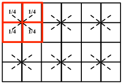
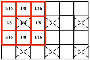
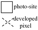
(a)	(b)

Figure 8: Neighborhood and filters for box down-sampling (a) and tent-down-sampling (b) for a factor 2, crosses represent the location of the predicted pixel.

IV-D3 Tent down-sampling

We now investigate more elaborated filters and particularly the problem of tent down-sampling (aka triangle down-sampling or bilinear down-sampling). This analysis enables to understand how it is possible to embed a message in the downscaled image using this particular filter, but it can also be adapted to all the class of linear filters, including for example the Gaussian kernel or the Lanczos kernel [32].

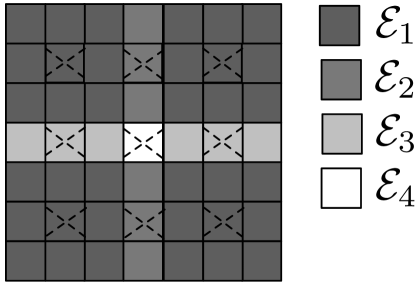
Figure 9: Embedding steps used for tent-down sampling: dark grey photo-sites are sampled during the first step, light grey photo-sites during the second step and white photo-sites during the last step.

As for color transform, we propose an embedding scheme that we believe is sub-optimal, i.e. that does’t convey the maximum payload but that ensures that the stego signal mimics correctly the sensor-noise. Without loss of generality the principle of the embedding scheme is explained for $c=2$ and in this case the tent filter and down-sampling process is illustrated on Figure 8(b).

This method starts by decomposing the down-scaled pixels into four disjoint lattices and associated subsets. Note that the embedding strategy is then similar to the ones designed to unable synchronization between embedding changes such as the “CMD” strategy or the “Sync” strategy [7, 8].

This decomposition is done in order to obtain developed pixels for which the stego signal is independently distributed conditionally to the neighborhood. On figure 8(b) we can see that the first and second developed pixels (represented by crosses) are not independant since 3 photo-sites contribute to the computation of both pixels, on the contrary the first and third pixels of the first row are independant.

The embedding procedure can be decomposed into four steps, each of them associated to a given subset of photo-sites.

In this section we adopt the following notations: indexes $i,j$ are centered on the pixel to develop ($\{-1,0,1\}$ represents respectively $\{1,2,3\}$ rows or columns), and the tent filter is denoted as a $3\times 3$ matrix with coefficient $c_{i,j}$. The four different subsets $\{\mathcal{E}_{1},\mathcal{E}_{2},\mathcal{E}_{3},\mathcal{E}_{4}\}$ of photo-sites are represented on Figure 9. Moreover $\overset{\uparrow}{s}$, $\overset{\downarrow}{s}$, $\overset{\leftarrow}{s}$ and $\overset{\rightarrow}{s}$ denotes stego signal added on the photo-sites related to neighboring developed pixels according to the $\uparrow,\downarrow,\leftarrow,\rightarrow$ directions. As an example it means that $s_{-1,0}=\overset{\uparrow}{s_{1,0}}$.

The embedding is sequentially performed in 4 steps:

1. The first step embeds part of the message (or generate the stego signal) into pixels belonging to $\text{$\mathcal{E}$}_{1}$. Because the subset $\mathcal{E}_{1}$ generates independent pixels, the stego signal in the developed domain is distributed as:

   $$\mathcal{N}(0,\sigma_{S1}^{2}),$$ (19)

   with $\sigma_{S1}^{2}=\sum_{i,j=-1}^{1}c_{i,j}^{2}\sigma_{S}^{2}(i,j)$. Applying results of III, one can compute the embedding probabilities, and the associated payload length associated to the pixels belonging to $\mathcal{E}_{1}$. In order to be able to sample the neighboring pixels, once an embedding change is done, we draw realizations of the 9 underlying photo-sites. This can be done by computing conditional probabilities or performing rejection sampling.

2. Developed pixels belonging to $\text{$\mathcal{E}$}_{2}$ have a sensor noise distributed according to the conditional density $f(\bar{s}|\overset{\leftarrow}{s}_{i-1,1},\overset{\leftarrow}{s}_{i,1},\overset{\leftarrow}{s}_{i+1,1},\overset{\rightarrow}{s}_{i-1,1},\overset{\rightarrow}{s}_{i,1},\overset{\rightarrow}{s}_{i+1,1})$ and consequently can be expressed as:

   $$\mathcal{N}(\mu_{S2},\sigma_{S2}^{2}),$$ (20)

   with $\mu_{S2}=\sum_{i=-1}^{1}c_{i,1}\overset{\leftarrow}{s}_{i,1}+\sum_{i=-1}^{1}c_{i,-1}\overset{\rightarrow}{s}_{i,-1}$ and $\sigma_{S2}^{2}=\sum_{i=-1}^{1}c_{i,0}^{2}\sigma_{S}^{2}(i,0)$. As for the first step, we can compute embedding probabilities and payload length for this subset. We can also draw the realizations of stego signal related to the 3 photo-sites belonging to this subset. Note that the same applies for steps 3 and 4.

3. Similarly pixels belonging to $\text{$\mathcal{E}$}_{3}$ have a sensor noise are distributed as:

   $$\mathcal{N}(\mu_{S3},\sigma_{S3}^{2}),$$ (21)

   with $\mu_{S3}=\sum_{j=-1}^{1}c_{1,j}\overset{\uparrow}{s}_{1,j}+\sum_{j=-1}^{1}c_{1,j}\overset{\downarrow}{s}_{1,j}$ and $\sigma_{S3}^{2}=\sum_{j=-1}^{1}c_{0,j}^{2}\sigma_{S}^{2}(0,j)$, and as for step 2, it is possible to draw realizations of the stego signal.

4. An finally, pixels belonging to $\text{$\mathcal{E}$}_{4}$ have a sensor noise distributed as:

   $$\mathcal{N}(\mu_{S4},\sigma_{S4}^{2}),$$ (22)

   with $\mu_{S4}=\sum_{j=-1}^{1}c_{1,j}\overset{\uparrow}{s}_{1,j}+\sum_{j=-1}^{1}c_{-1,j}\overset{\downarrow}{s}_{-1,j}+c_{0,1}\overset{\leftarrow}{s}_{0,1}+c_{0,-1}\overset{\rightarrow}{s}_{0,-1}$ and $\sigma_{S4}^{2}=c_{0,0}^{2}\sigma_{S}^{2}(0,0)$. For this last step, notice that only one photo-site is drawn.

Note that since $H(\bar{S}|\overset{\leftarrow}{S}_{i-1,1},\overset{\leftarrow}{S}_{i,1},\overset{\leftarrow}{S}_{i+1,1},\overset{\rightarrow}{S}_{i-1,1},\overset{\rightarrow}{S}_{i,1},\overset{\rightarrow}{S}_{i+1,1})\leq H(\bar{S})$, the payload length embedded during steps 4 is smaller than the payload length embedded during 2 and 3, which is smaller than the payload length embedded during step 1.

V Experimental results

The goal of this section is to benchmark the detectability of NS, to compare it with other steganographic schemes using same embedding payload, but also to analyze the effects of developing operations w.r.t. both detectability and embedding rates.

V-A Generation of “MonoBase”

In order to benchmark the concept of embedding using cover-source switching, we needed to acquire different sources providing OOC images. To do so we conducted the following experiment: using a Leica M Monochrome Type 230 camera, we captured two sets of 172 pictures taken at 1000 ISO or 1250 ISO. In order to have large diversity of contents most of the pictures were captured using a 21mm lens in a urban environment, or a 90mm lens capturing cluttered places.

The exposure time was set to automatic, with exposure compensation set to -1 in order to prevent over-exposure. A tripod was used so that pictures for the two sensitivity settings correspond to the same scene. Each RAW picture was then converted into a 16-bit PGM picture using the same conversion operation as the one presented in section II-B and each $5212\times 3472$ picture was then cropped into $6\times 10=60$ PGM pictures of size $512\times 512$ to obtain two sets of 10320 16-bit PGM pictures. We consequently end up with a database of a similar size than BOSSBase, with pictures of same size that contrary to un-cropped pictures can be quickly processed either for embedding or feature extraction. This database called MonoBase is downloadable here [33]. Figure 7 shows several images of MonoBase.

V-B Benchmark setup

For all the following experiments, we adopt the Spatial Rich Model feature sets [34] combined with the Ensemble Classifier (EC) [35] and we report the average total error $P_{E}=\min((P_{FA}+P_{MD})/2)$ obtained after training the EC on 10 different training/testing sets divided in 50/50. The stego database consists of images captured at 1000 ISO perturbed with an embedding noise mimicking 1250 ISO, and the cover database consists of images captured at 1250 ISO. In order to have an effect equivalent with the principle of training using pairs of cover and stego images, the pairs are constructed using one couple of images capturing the same scene.

The parameters of the stego signal are denoted $a"$ and $b"$ with the relations $a"=a^{\prime}(2^{N_{b}}-1)$ and $b"=b^{\prime}(2^{N_{b}}-1)^{2}$, where $a^{\prime}$ and $b^{\prime}$ are computed using normalized image values in order to be resolution independant (see section III-A). $N_{b}=16$ when the cover image coded in 16-bit is used and $N_{b}=8$ when the stego image is directly generated from the 8-bit representation of the cover image.

V-C Basic developing and comparison with S-Uniward

We first benchmark the scheme proposed in section III and generate 8-bit stego images where the stego signal is generated according to the embedding probabilities computed in 10. Like all the modern steganographic schemes, we forbid embeddings by attributing wet pixels to cover pixels saturated at 0 or 255. We also propose a variation of NS where the dark pixels, i.e. the pixels of the cover have the lowest value after 8-bits quantization, are also wet. This strategy, even if developed independently, is similar to the one recently proposed in [36]. For NS, we used the same values that the ones estimated in section II, i.e. $a"=2.1\,10^{-5}$ and $b"=8.4\,10^{-7}$.

The two first columns of table I show the high undetectability of the proposed scheme, and the small improvement associated to wet the dark pixels. We note that we are still around $7\%$ from random guessing, and we think that it can be due to the different assumption presented in section III, particularly the fact that the quantization noise is ignored.

	NS	NS	SUni-SI	SUni	1000 ISO
	wo wet dark		1000 ISO	1000 ISO	vs 1250 ISO
$P_{E}$	41.0%	42.8%	18.2%	12.3%	26.0%

Table I: Results and comparison with S-Uniward on MonoBase 1000 ISO.

Figure 10 depicts the histogram of the embedding rate ($E_{r}$) on MonoBase. We can see that most of the embedding rates are relatively high for steganography with an average of 1.24 bpp for this base. Note that on MonoBase, most of the images are under-exposed, which means that the average embedding rate should higher for a “typical” database. It is important to point here that contrary to most of the steganographic schemes, the current implementation of NS does not enable an embedding at a constant payload, but this as the price of high undetectability.

Figure 10: Histogram of the embedding rates for MonoBase with covers-source switching from 1000 ISO to 1250 ISO. $\mathrm{E}[E_{r}]=1.24\,\mathrm{pbb}$. .

The two next columns of Figure 10 compare the performances of NS with S-Uniward. We choose this steganographic scheme because of its excellent performances and because it has recently been tuned to take into account the side-information offered by 16-bit to 8-bit conversion [13]. The two implementations of S-Uniward where benchmarked on MonoBase 1000 ISO on a fixed embedding rate equal to the average embedding rate of NS, but we obtained similar performances on MonoBase 1250 ISO. This scheme, even if excellent at deriving embedding costs and targeting textured regions of the image, cannot compete with an embedding scheme which is model-based and which enable cover-source switching like NS.

The last column compare our steganalysis task with the classification task of separating images captured at 1000 ISO from image captured at 1250 ISO. We can see that this task using the SRM is not an easy task since the error probability is still rather important.

Figure 11 depicts the sensitivity of our scheme to the estimation of the sensor noise by computing the classification error for different values of $a"$ and $b"$. We can see that the estimation of the sensor noise is rather important, going from example from $a"=2.1\,10^{-5}$ to $a"=10^{-5}$ increases the detectability by approximately 5%.

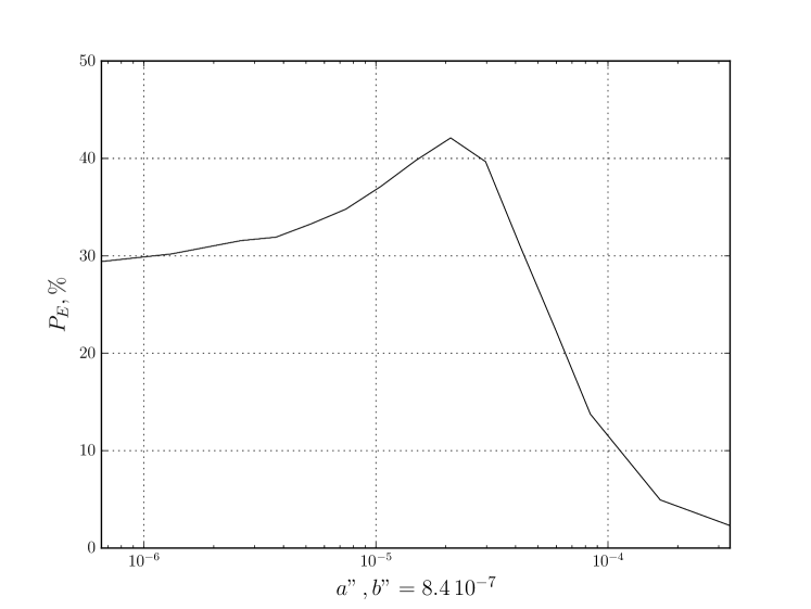
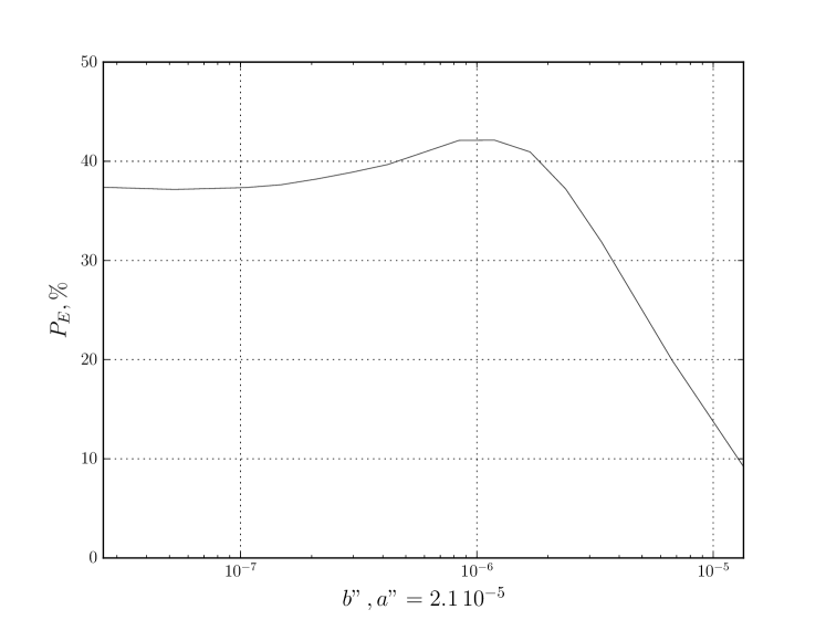
Figure 11: Sensitivity w.r.t. the model parameters $a"$ and $b"$.

V-D Results with 8-bit embedding

	NS	NS 8-bits
$P_{E}$	42.8%	18.4%

Table II: Impact of using the side-information of NS.

Table II presents results when the embedding is directly performed on 8-bit cover images and we can notice that in this case the scheme becomes highly detectable. We explain this problem by the fact that dark regions, which undergo both stego signal and sensor-noise of small variance are not modified in a natural way. These regions are especially sensitive to steganalysis because they are less noisy than bright regions, and because the value of the photo-site before 16-bit/8-bit conversion highly impact the sign of the embedding change in this case. Figure 12 show the embedding change for a portion of a cover image having dark areas and we can see that for the 8-bit embedding, the number of embedding changes are less important since the dithering effect offered by the use of the 16-bit image is lost here (the sensor noise is in this case centered directly on the quantization cell). Trying to improve NS in this practical setup is left for future researches.

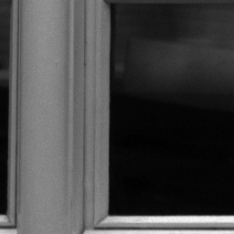
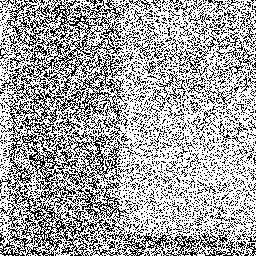
(a)	(b)	(c)

Figure 12: Portion of an image (a) and locations of embedding changes when 16-bit to 8-bit is used (b) and when it is not used (c) (for better rendering, inactivate interpolation on your pdf viewer).

V-E Gamma correction

Table III shows the detectability results of NS once gamma correction is performed during the developing step both on cover and on stego images. 16-bit cover images are used. Since the model of the stego signal is adapted to feat the model of the sensor-noise after the gamma correction (see IV-A) we can check that the undetectability of NS is still high.

We see also that on MonoBase the embedding rate increases w.r.t. the parameter $\gamma$. This is because for $\gamma>1$ the variance of the stego signal increases for small photo-site values and decreases for large photo-site values. The inverses occurs for $\gamma<1.$ In the first case this is due to the convexity of the transform, in the second case to the concavity of the transform. On a database only composed of bright images, the effect would be the opposite.

$\gamma$	2.5	2	1.5	1	0.5
$P_{E}$	40.2%	42.1%	40.7%	42.2%	43.3%
$E_{r}$(bpp)	1.61	1.62	1.55	1.24	0.5

Table III: Performances of NS after Gamma correction.

V-F Downsampling

Table IV presents the detectability results after downsampling the images of a factor 2 (because the images were already really small we did not use $c>2$). We can notice the detectability is smaller after down-sampling, which is probably due to the effect of the square root law [37].

	NS	NS	NS	NS
		Sub-sampling	$c=2$, Box	$c=2$, Tent
$P_{E}$	42.8%	48%	47.7%	48.0%

Table IV: Detectably after x2 downsampling.

Figure 13 presents the evolution of the embedding rates computed using the densities of the stego signal for the three down-sampling methods presented in (see IV-D) for an image having photo-sites uniformly and independently distributed between 0 and $2^{16}-1$.

We can notice that the embedding rates rapidly decrease w.r.t. the scaling factor for Box or Tent downscaling. The rate is constant for classical sub-sampling but this method generates aliasing and is never used in practice. If we for example look at the typical down-scaling operation used in BOSS-Base, a 18MP image (3840 x 2592) was downsampled with c=5, which lead in these case to $E_{r}\thickapprox 0.4\,\mathrm{pbb}$ for Box downsampling and $E_{r}\thickapprox 0.2\,\mathrm{pbb}$ for Tent downsampling. Compared with the initial embedding rate of 1.8 pbb, the reduction is rather important. Note that for a given detectability constraint, the embedder can always increase the values of $a"$ and $b"$ to increase the payload, or change the cover-source switching setup by using $ISO_{1}<1000$ or $ISO_{2}>1250$.

We can draw two remarks comparing with the literature on steganography:

1. The evolution of the detectability is perfectly inline with the analyzed effect of rescaling in steganalysis [38] (see for example Figure 1 of [38]) which outlines that the Tent kernel is more detectable than the Box kernel.

2. The generation of the stego signal after resampling implies computation of conditional probabilities which force the embedding scheme to correlate the neighboring embedding changes, which is also inline with the Synch or CMD strategies presented in [7, 8].

Figure 13: Embedding rate vs scaling factor, 1000 ISO toward 1250 ISO embedding for a cover image uniformly distributed, $a^{\prime}=2.1\times 10^{-5}$,$b^{\prime}=8.4\times 10^{-7}$.

VI Another strategy: cover-source perturbation

We want to mention alternative strategy to cover-source switching which is cover-source perturbation. In this case the embedding does not mimic another cover-source but just slightly perturbs it. This can simply done by setting $b"=0$, setting $a"$ and comparing cover images with stego images with the same sensitivity (here 1000 ISO), this way the stego signal slightly perturbs the sensor-noise. The advantage of cover-source perturbation is the fact that is doesn’t require to model the source sensor noise which can be very interesting in practice.

We present results related to cover-source perturbation in Table V which depicts the evolution of the detection error and the embedding w.r.t. $a"$ when both cover images are at 1000 ISO. We can notice that cover-source perturbation may offer undetectability but at the price of a smaller embedding rate. For example for the same $P_{E}$ as NS with cover-source switching, the embedding rate is roughly divided by 3.

a”	$4\,10^{-7}$	$1.5\,10^{-6}$	$6.3\,10^{-6}$	$2.5\,10^{-5}$	$10^{-4}$
$P_{E}$	46.2%	45.5%	41.4%	24.7%	5.4%
$E_{r}$ (bpp)	0.16	0.32	0.63	1.19	1.98

Table V: Cover-source perturbation, comparison with covers at 1000 ISO.

VII Conclusions and perspectives

We have proposed in this paper a new methodology for steganography based on the principle of cover-source switching, i.e. the fact that the embedding should mimics the switching from one cover-source to another. The scheme we presented scheme (NS) used the sensor noise to model one source and message embedding is performed by generating a suited stego signal which enables the switch. This method, in order to provide good undetectability performances while proposing high embedding rates, has to use RAW images as inputs. We also show in the paper how to handle different steps of image developing, including quantization, gamma correction, color transforms and rescaling operations.

In future works we want also to investigate other setups for NS steganography, such as choosing other ISO parameters and different camera models. It will also be important to try to improve direct embedding on 8-bit images and to address more practical implementation such as embedding in the JPEG-domain.

From the adversary point of view, we would like to see if more appropriate feature could be designed for this category of schemes, this kind of features should not be sensitive only to image variation, but also to the sensor noise whose variance is function of the pixel luminance.

Another track of research is to consider other ways to perform cover-source switching (or cover-source perturbation, see section VI), where the source can be represented here by, for example, the demosaicing algorithm. Since the behavior of demosaicing algorithms fluctuates a lot in textures, we think that this strategy would generate embedding changes that are closer to the ones used currently by other steganographic methods.

Finally we hope that this methodology will page the road for new directions in steganography.

VIII Acknowledgments

The author would like to thank Boris Valet for his work on sensor noise estimation, Cyrille Toulet and Matthieu Marquillie for their help on the Univ-lille HPC, Remi Bardenet for his help on sampling strategies, Tomas Pevny and Andrew Ker for their inspiring conversations of the definition of the source, and CNRS for a supporting grant on cyber-security.

References

- [1] C. Cachin, “An information-theoretic model for steganography,” in Information Hiding: Second International Workshop IHW’98, Portland, Oregon, USA, April 1998.
- [2] P. Sallee, “Model-based steganography,” in International Workshop on Digital Watermarking (IWDW), LNCS, vol. 2, 2003.
- [3] T. Pevny, T. Filler, and P. Bas, “Using high-dimensional image models to perform highly undetectable steganography,” in Information Hiding 2010, 2010.
- [4] V. Sedighi, R. Cogranne, and J. Fridrich, “Content-adaptive steganography by minimizing statistical detectability,” vol. 11, no. 2, Feb 2016, pp. 221 – 234.
- [5] V. Holub, J. Fridrich, and T. Denemark, “Universal distortion function for steganography in an arbitrary domain,” EURASIP Journal on Information Security, vol. 2014, no. 1, pp. 1–13, 2014.
- [6] B. Li, M. Wang, J. Huang, and X. Li, “A new cost function for spatial image steganography,” in Image Processing (ICIP), 2014 IEEE International Conference on. IEEE, 2014, pp. 4206–4210.
- [7] T. Denemark, V. Sedighi, V. Holub, R. Cogranne, and J. Fridrich, “Selection-channel-aware rich model for steganalysis of digital images,” in IEEE Workshop on Information Forensic and Security, Atlanta, GA, 2014.
- [8] B. Li, M. Wang, X. Li, S. Tan, and J. Huang, “A strategy of clustering modification directions in spatial image steganography,” Information Forensics and Security, IEEE Transactions on, vol. 10, no. 9, pp. 1905–1917, 2015.
- [9] W. Tang, B. Li, W. Luo, and J. Huang, “Clustering steganographic modification directions for color components,” 2016.
- [10] T. Filler, J. Judas, and J. Fridrich, “Minimizing additive distortion in steganography using syndrome-trellis codes,” Information Forensics and Security, IEEE Transactions on, vol. 6, no. 3, pp. 920–935, 2011.
- [11] P. Wang, H. Zhang, Y. Cao, and X. Zhao, “Constructing near-optimal double-layered syndrome-trellis codes for spatial steganography,” in ACM workshop on Information hiding and multimedia security. ACM, 2016.
- [12] J. Fridrich, M. Goljan, and D. Soukal, “Perturbed quantization steganography with wet paper codes,” in Proceedings of the 2004 workshop on Multimedia and security. ACM, 2004, pp. 4–15.
- [13] T. Denemark and J. Fridrich, “Side-informed steganography with additive distortion,” in IEEE WIFS, 2016.
- [14] P. Bas, T. Filler, and T. Pevny, “"Break Our Steganographic System": The Ins and Outs of Organizing BOSS,” in INFORMATION HIDING, ser. Lecture Notes in Computer Science, vol. 6958/2011, Czech Republic, Sep. 2011, pp. 59–70.
- [15] J. Fridrich, J. Kodovskỳ, V. Holub, and M. Goljan, “Breaking hugo–the process discovery,” in Information Hiding. Springer, 2011, pp. 85–101.
- [16] A. D. Ker and T. Pevny, “The steganographer is the outlier: realistic large-scale steganalysis,” 2014.
- [17] “http://www.cybercom.net/ dcoffin/dcraw/.”
- [18] “https://sourceforge.net/projects/exiftool/.”
- [19] E. Franz and A. Pfitzmann, “Steganography secure against cover-stego-attacks,” in Information Hiding. Springer, 1999, pp. 29–46.
- [20] E. Franz and A. Schneidewind, “Pre-processing for adding noise steganography,” in Information Hiding, 7th International Workshop, 2005, pp. 189–203.
- [21] T. Holotyak, J. Fridrich, and S. Voloshynovskiy, “Blind statistical steganalysis of additive steganography using wavelet higher order statistics,” in Communications and Multimedia Security, vol. 3677, 2005, pp. 273–274.
- [22] A. Foi, M. Trimeche, V. Katkovnik, and K. Egiazarian, “Practical poissonian-gaussian noise modeling and fitting for single-image raw-data,” Image Processing, IEEE Transactions on, vol. 17, no. 10, pp. 1737–1754, 2008.
- [23] A. Foi, S. Alenius, V. Katkovnik, and K. Egiazarian, “Noise measurement for raw-data of digital imaging sensors by automatic segmentation of nonuniform targets,” IEEE Sensors Journal, vol. 7, no. 10, pp. 1456–1461, 2007.
- [24] E. M. V. Association et al., “Standard for characterization of image sensors and cameras,” EMVA Standard, vol. 1288, 2010.
- [25] T. Qiao, F. Retraint, R. Cogranne, and T. H. Thai, “Source camera device identification based on raw images,” in Image Processing (ICIP), 2015 IEEE International Conference on, Sept 2015, pp. 3812–3816.
- [26] T. H. Thai, R. Cogranne, and F. Retraint, “Camera model identification based on the heteroscedastic noise model,” IEEE Transactions on Image Processing, vol. 23, no. 1, pp. 250–263, Jan 2014.
- [27] E. Chang, S. Cheung, and D. Y. Pan, “Color filter array recovery using a threshold-based variable number of gradients,” in Electronic Imaging’99. International Society for Optics and Photonics, 1999, pp. 36–43.
- [28] C. kai Lin, “Pixel grouping,” http://sites.google.com/site/chklin/demosaic, 2010.
- [29] K. Hirakawa and T. W. Parks, “Adaptive homogeneity-directed demosaicing algorithm,” IEEE Transactions on Image Processing, vol. 14, no. 3, pp. 360–369, 2005.
- [30] , “Libraw raw image decoder,” http://www.libraw.org, 2010.
- [31] “Foveon x3 sensor,” https://en.wikipedia.org/wiki/Foveon_X3_sensor, March 2016.
- [32] K. Turkowski, “Filters for common resampling tasks,” in Graphics gems. Academic Press Professional, Inc., 1990, pp. 147–165.
- [33] P. Bas, “Monobase,” http://patrickbas.ec-lille.fr/MonoBase/, July 2016.
- [34] J. Fridrich and J. Kodovsky, “Rich models for steganalysis of digital images,” Information Forensics and Security, IEEE Transactions on, vol. 7, no. 3, pp. 868–882, 2012.
- [35] J. Kodovsky, J. Fridrich, and V. Holub, “Ensemble classifiers for steganalysis of digital media,” Information Forensics and Security, IEEE Transactions on, vol. 7, no. 2, pp. 432–444, 2012.
- [36] V. Sedighi and J. Fridrich, “Effect of saturated pixels on security of steganographic schemes for digital images,” in Proc. if ICIP, Singapore, Oct. 2016.
- [37] A. D. Ker, T. Pevnỳ, J. Kodovskỳ, and J. Fridrich, “The square root law of steganographic capacity,” in Proceedings of the 10th ACM workshop on Multimedia and security. ACM, 2008, pp. 107–116.
- [38] J. Kodovsky and J. Fridrich, “Steganalysis in resized images,” in Acoustics, Speech and Signal Processing (ICASSP), 2013 IEEE International Conference on. IEEE, 2013, pp. 2857–2861.