Lecture notes on stochastic models in systems biology

Abstract

These notes provide a short, focused introduction to modelling stochastic gene expression, including a derivation of the master equation, the recovery of deterministic dynamics, birth-and-death processes, and Langevin theory. The notes were last updated around 2010 and written for lectures given at summer schools held at McGill University’s Centre for Non-linear Dynamics in 2004, 2006, and 2008.

Introduction

A system evolves stochastically if its dynamics is partly generated by a force of random strength or by a force at random times or by both. For stochastic systems, it is not possible to exactly determine the state of the system at later times given its state at the current time. Instead, to describe a stochastic system, we use the probability that the system is in a certain state and can predict how this probability changes with time. Calculating this probability is often difficult, and we usually focus on finding the moments of the probability distribution, such as the mean and variance, which are commonly measured experimentally.

Any chemical reaction is stochastic. Reactants come together by diffusion, their motion driven by collisions with other molecules. Once together, these same collisions alter the internal energies of the reactants, and so their propensity to react. Both effects cause individual reaction events to occur randomly.

Is stochasticity important in biology? Intuitively, stochasticity is only significant when typical numbers of molecules are low. Then individual reactions, which at most change the numbers of molecules by one or two, matter. Low numbers are frequent in vivo: gene copy number is typically one or two, and transcription factors often number in the tens, at least in bacteria. There are now many reviews on biochemical stochasticity[1, 2, 3, 4].

Unambiguously measuring stochastic gene expression, however, can be challenging [5]. Naively, we could place Green Fluorescent Protein (GFP) on a bacterial chromosome downstream of a promoter that is activated by the system of interest. By measuring the variation in fluorescence across a population of cells, we could quantify stochasticity. Every biochemical reaction, however, is potentially stochastic. Fluorescence variation could be because of stochasticity in the process under study or could result from the general background ‘hum’ of stochasticity: stochastic effects in ribosome synthesis could lead to different numbers of ribosomes and so to differences in gene expression in each cell; stochastic effects in the cell cycle machinery may desynchronize the population; stochastic effects in signaling networks could cause each cell to respond uniquely, and so on.

Variation has then two classes: intrinsic stochasticity, the stochasticity inherent in the dynamics of the system and that arises from fluctuations in the timing of individual reactions, and extrinsic stochasticity, the stochasticity originating from reactions of the system of interest with other stochastic systems in the cell or its environment [6, 5]. In principle, intrinsic and extrinsic stochasticity can be measured by creating a copy of the network of interest in the same cellular environment as the original network [5]. We can define intrinsic and extrinsic variables for the system of interest, with fluctuations in these variables together generating intrinsic and extrinsic stochasticity [6]. The intrinsic variables of a system will typically specify the copy numbers of the molecular components of the system. For gene expression, the level of occupancy of the promoter by transcription factors, the numbers of mRNA molecules, and the number of proteins are all intrinsic variables. Imagining a second copy of the system – an identical gene and promoter elsewhere in the genome – then the instantaneous values of the intrinsic variables of this copy of the system will usually differ from those of the original system. At any point in time, for example, the number of mRNAs transcribed from the first copy of the gene will usually be different from the number of mRNAs transcribed from the second copy. Extrinsic variables, however, describe processes that equally affect each copy of the system. Their values are therefore the same for each copy. For example, the number of cytosolic RNA polymerases is an extrinsic variable because the rate of gene expression from both copies of the gene will increase if the number of cytosolic RNA polymerases increases and decrease if the number of cytosolic RNA polymerases decreases. In contrast, the number of transcribing RNA polymerases is an intrinsic variable because we expect the number of transcribing RNA polymerases to be different for each copy of the gene at any point in time.

Stochasticity is quantified by measuring an intrinsic variable for both copies of the system. For gene expression, the number of proteins is typically measured by using fluorescent proteins as markers [7, 5, 8, 9]. Imaging a population of cells then allows estimation of the distribution of protein levels at steady-state. Fluctuations of the intrinsic variable will in vivo have both intrinsic and extrinsic sources. The number of proteins will fluctuate because of intrinsic stochasticity generated during gene expression, but also because of stochasticity in, for example, the number of cytosolic RNA polymerases or ribosomes or proteosomes. We will use the term ‘noise’ to mean an empirical measure of stochasticity defined by the coefficient of variation (the standard deviation divided by the mean) of a stochastic process. An estimate of intrinsic stochasticity is the intrinsic noise which is defined as a measure of the difference between the value of an intrinsic variable for one copy of the system and its counterpart in the second copy. For gene expression, typically the intrinsic noise is the mean absolute difference (suitably normalized) at steady-state between the number of proteins expressed from one copy of the gene and the number of proteins expressed from the other copy [5]. Such a definition supports the intuition that intrinsic fluctuations cause variation in one copy of the system to be uncorrelated with variation in the other copy. Extrinsic noise is defined as the correlation coefficient between the intrinsic variable of one copy of the system and its counterpart for the other copy because extrinsic fluctuations equally affect both copies of the system and consequently cause correlations between variation in one copy and variation in the other. The intrinsic and extrinsic noise should be related to the coefficient of variation of the intrinsic variable of the original system of interest. This so-called total noise is given by the square root of the sum of the squares of the intrinsic and the extrinsic noise [6].

Such two-colour measurements of stochasticity have been applied to bacteria and yeast where gene expression has been characterized by using two copies of a promoter placed in the genome with each copy driving a distinguishable allele of Green Fluorescent Protein [5, 9]. Both intrinsic and extrinsic noise can be substantial giving, for example, a total noise of around 0.4, and so the standard deviation of protein numbers is 40% of the mean. Extrinsic noise is usually higher than intrinsic noise. There are some experimental caveats: both copies of the system should be placed ‘equally’ in the genome so that the probabilities of transcription and replication are equal. This ‘equality’ is perhaps best met by placing the two genes adjacent to each other [5]. Although conceptually there are no difficulties, practically problems arise with feedback. If the protein synthesized in one system can influence its own expression, the same protein will also influence expression in a second copy of the system. The two copies of the system have lost the (conditional) independence they require to be two simultaneous measurements of the same stochastic process.

A stochastic description of chemical reactions

For any network of chemical reactions, the lowest level of description commonly used in systems biology is the chemical master equation. This equation assumes that the system is well-stirred and so ignores spatial effects. It governs how the probability of the system being in any particular state changes with time. A system state is defined by the number of molecules present for each chemical species, and it will change every time a reaction occurs. From the master equation we can derive the deterministic approximation (a set of coupled differential equations) which is often used to describe system dynamics. The dynamics of the mean of each chemical species approximately obeys these deterministic equations as the numbers of molecules of all species increase [10, 11]. The master equation itself is usually only solvable analytically for linear systems: systems having only first-order chemical reactions.

Nevertheless, several approximations exist, all of which exploit the tendency of fluctuations to decrease as the numbers of molecules increase. The most systematic is the linear noise approach of van Kampen [12]. If the concentration of each chemical species is fixed, then changing the system volume, $\Omega$, alters the number of molecules of every chemical species. The linear noise approximation is based on a systematic expansion of the master equation in the inverse of the system volume, $\Omega^{-1}$. It leads to diffusion-like equations that accurately describe small fluctuations around any stable attractor of the system. For systems that tend to steady-state, a Langevin approach is also often used [13, 14, 15]. Here additive, white stochastic terms are included in the deterministic equations, with the magnitude of these terms being determined by the chemical reactions. At steady-state and for sufficiently high numbers of molecules, the Langevin and linear noise approaches are equivalent.

Unfortunately, all these methods become intractable, in general, once the number of chemical species in the system reaches more than three (we then need to analytically calculate the inverse of at least a $4\times 4$ matrix or its eigenvalues). Rather than numerically solve the master equation, the Gillespie algorithm [16], a Monte Carlo method, is often used to simulate intrinsic fluctuations by generating one sample time course from the master equation. By doing many simulations and averaging, the mean and variance for each chemical species can be calculated as a function of time. Extrinsic fluctuations can be modelled as fluctuations in the parameters of the system, such as the kinetic rates [17, 18]. They can be included by a minor modification of the Gillespie algorithm that feeds in a pre-simulated time series of extrinsic fluctations and so generates both intrinsic and extrinsic fluctuations [18].

Here we will introduce the master equation and briefly discuss the Gillespie algorithm.

The master equation

Once molecules can react, the intrinsic stochsasticity destroys any certainty of the numbers and types of molecules present, and we must adopt a probabilistic description. For example, a model of gene expression is given by

$$\ce{->[k]C->[d]0}$$

where protein $C$ is synthesized on average every $1/k$ seconds and degrades on average every $1/d$ seconds. The reactions can be described by the probability

$${\cal P}(\mbox{$n$ molecules of $C$ at time $t$})$$

and how this probability evolves with time. Each reaction rate is interpreted as the probability per unit time of the appropriate reaction.

We will write $P_{n}(t)$ for the probability that $n$ proteins exist at time $t$ and consider the reactions that might have occurred just prior to having $n$ molecules of protein. Let $\delta t$ be a time interval small enough so that at most only one reaction can occur. If there are $n$ proteins at time $t+\delta t$, then if a protein was synthesized during the interval $\delta t$, there must have been $n-1$ proteins at time $t$. The probability of synthesis is

$${\cal P}({\rm synthesis})=k\delta t$$ (1)

which is independent of the number of proteins present. If we have $n$ proteins at time $t+\delta t$ and a protein was degraded during the interval $\delta t$, however, there must have been $n+1$ proteins at time $t$. The probability of degradation is

$${\cal P}({\rm degradation})=(n+1)d\delta t.$$ (2)

Neither synthesis nor degradation may have occurred during $\delta t$. The number of proteins will be unchanged, which occurs with probability

$${\cal P}(\mbox{no reaction})=1-k\delta t-nd\delta t.$$ (3)

Notice that the probability of a protein degrading is $nd\delta t$ because $n$ proteins must have existed at time $t$.

Putting these probabilities together, we can the master equation describing the time evolution of $P_{n}(t)$. Writing

$$P_{n}(t+\delta t)=P_{n-1}(t)k\delta t+P_{n+1}(t)d(n+1)\delta t+P_{n}(t)(1-k\delta t-nd\delta t).$$ (4)

dividing through by $\delta t$ and taking the limit $\delta t\rightarrow 0$ gives

$$\frac{\partial}{\partial t}P_{n}=k\Bigl{[}P_{n-1}-P_{n}\Bigr{]}-d\Bigl{[}nP_{n}-(n+1)P_{n+1}\Bigr{]}$$ (5)

Eq. 5 is an example of a master equation: all the moments of the probability distribution $P_{n}(t)$ can be derived from it.

Consider now a binary reaction:

$$\ce{A+B->[f]C}$$ (6)

where $A$ and $B$ bind irreversibly to form complex $C$ with probability $f$ per unit time. Suppose further that individual $C$ molecules degrade with probability $d$ per unit time

$$\ce{C->[d]0}$$

The state of the system is then described by

$${\cal P}(\mbox{$n_{A}$ molecules of $A$, $n_{B}$ molecules of $B$, and $n_{C}$ molecules of $C$ at time $t$})$$

which we will write as $P_{n_{A},n_{B},n_{C}}(t)$. We again consider a time interval $\delta t$ small enough so that at most only one reaction can occur. If the system at time $t+\delta t$ has $n_{A}$, $n_{B}$, and $n_{C}$ molecules of $A$, $B$, and $C$, then if reaction $f$ occurred during the interval $\delta t$, the system must have been in the state $n_{A}+1$, $n_{B}+1,$ and $n_{C}-1$ at time $t$. The probability of this reaction is

$${\cal P}(\mbox{$f$ reaction})=f(n_{A}+1)(n_{B}+1)\delta t.$$ (7)

Alternatively, reaction $d$ could have occurred during $\delta t$ and so the system then must have been in the state $n_{A}$, $n_{B}$, and $n_{C}+1$ at time $t$. Its probability is

$${\cal P}(\mbox{$d$ reaction})=d(n_{C}+1)\delta t.$$ (8)

Finally, no reaction may have occurred at all, and so the system would be unchanged at $t$ (in the state $n_{A}$, $n_{B}$, and $n_{C}$):

$${\cal P}(\mbox{no reaction})=1-fn_{A}n_{B}\delta t-dn_{C}\delta t.$$ (9)

Thus we can find the master equation by writing

$$P_{n_{A},n_{B},n_{C}}(t+\delta t)=$$ (10)

$$P_{n_{A}+1,n_{B}+1,n_{C}-1}(t)(n_{A}+1)(n_{B}+1)f\delta t+P_{n_{A},n_{B},n_{C}+1}(t)(n_{C}+1)d\delta t$$

$$+P_{n_{A},n_{B},n_{C}}(t)\Bigl{[}1-n_{A}n_{B}f\delta t-n_{C}d\delta t\Bigr{]}$$

or

$$\frac{\partial}{\partial t}P_{n_{A},n_{B},n_{C}} = f\Bigl{[}(n_{A}+1)(n_{B}+1)P_{n_{A}+1,n_{B}+1,n_{C}-1}-n_{A}n_{B}P_{n_{A},n_{B},n_{C}}\Bigr{]}$$ (11)

$$-d\Bigl{[}n_{C}P_{n_{A},n_{B},n_{C}}-(n_{C}+1)P_{n_{A},n_{B},n_{C}+1}\Bigr{]}$$

in the limit of $\delta t\rightarrow 0$.

The definition of noise

Noise is typically defined as the coefficient of variation: the ratio of the standard deviation of a distribution to its mean. We will denote noise by $\eta$:

$$\eta=\frac{\sqrt{\langle N^{2}\rangle-\langle N\rangle^{2}}}{\langle N\rangle}$$ (12)

for a random variable $N$. The noise is dimensionless and measures the magnitude of a typical fluctuation as a fraction of the mean.

Example: A birth-and-death processes

The model of gene expression

$$\ce{->[k]C->[d]0}$$ (13)

is a birth-and-death process. Proteins can only be synthesized (born) or degrade (die). We will solve the master equation for this system, Eq. 5, using a moment generating function.

The moment generating function for a probability distribution $P_{n}(t)$ is defined as

$$F(z,t)=\sum_{n=0}^{\infty}z^{n}P_{n}(t)$$ (14)

and can be thought of as a discrete transform. Differentiating the moment generating function with respect to $z$ gives

$$\frac{\partial F}{\partial z} = \sum_{n=0}^{\infty}nz^{n-1}P_{n}$$ (15)

$$\frac{\partial^{2}F}{\partial z^{2}} = \sum_{n=0}^{\infty}n(n-1)z^{n-2}P_{n}.$$ (16)

The generating function and its derivatives have useful properties because of their dependence on the probability distribution $P_{n}(t)$:

$$F(z=1,t) = \sum_{n=0}^{\infty}P_{n}(t)=1$$ (17)

$$\frac{\partial F}{\partial z}(z=1,t) = \sum_{n=0}^{\infty}nP_{n}(t)=\langle n(t)\rangle$$ (18)

$$\frac{\partial^{2}F}{\partial z^{2}}(z=1,t) = \sum_{n=0}^{\infty}n(n-1)P_{n}(t)=\langle n^{2}(t)\rangle-\langle n(t)\rangle.$$ (19)

Finding $F(z,t)$ therefore allows us to calculate all the moments of $P_{n}(t)$: $F(z,t)$ is called the moment generating function.

The master equation can be converted into a partial differential equation for the moment generating function. Multiplying (5) by $z^{n}$ and summing over all $n$ gives

$$\frac{\partial F}{\partial t} = k\sum_{n}z^{n}P_{n-1}-kF-d\sum_{n}nz^{n}P_{n-1}+d\sum_{n}(n+1)z^{n}P_{n+1}$$ (20)

$$= kz\sum_{n}z^{n-1}P_{n-1}-kF-dz\sum_{n}nz^{n-1}P_{n}+d\sum_{n}(n+1)z^{n}P_{n+1}$$

where we have factored $z$ out of some of the sums so that we can use (14) and (15). With these results and setting $P_{n}=0$ if $n<0$, we can write

$$\frac{\partial F}{\partial t}=kzF-F-dz\frac{\partial F}{\partial z}+d\frac{\partial F}{\partial z}$$ (21)

or

$$\frac{\partial F}{\partial t}=(z-1)\left(kF-d\frac{\partial F}{\partial z}\right).$$ (22)

This first order partial differential equation can be solved in general using the method of characteristics [12].

We will solve (22) to find the steady-state probability distribution of protein numbers. At steady-state, $P_{n}(t)$ is independent of time and so $\frac{\partial F}{\partial t}=0$ from (14). Consequently, (22) becomes

$$\frac{\partial F}{\partial z}=\frac{k}{d}F$$ (23)

which is an ordinary differential equation. This equation has a solution

$$F(z)=C{\rm e}^{\frac{k}{d}z}$$ (24)

for some constant $C$. This constant can be determined from (17), implying

$$F(z)={\rm e}^{\frac{k}{d}(z-1)}.$$ (25)

By differentiation (25) with respect to $z$ and using (18) and (19), the moments of $n$ can be calculated. For this case, we can Taylor expand (25) and find the probability distribution $P_{n}$ by comparing the expansion with (14). Expanding gives

$$F(z)={\rm e}^{-\frac{k}{d}}\sum_{n=0}^{\infty}\frac{\left(k/d\right)^{n}}{n!}z^{n}$$ (26)

implying that the steady-state probability of having $n$ proteins is

$$P_{n}={\rm e}^{-k/d}\frac{\left(k/d\right)^{n}}{n!}$$ (27)

which is a Poisson distribution. The first two moments are

$$\langle n\rangle = k/d$$

$$\langle n^{2}\rangle-\langle n\rangle^{2} = k/d\;=\;\langle n\rangle$$ (28)

and consequently the noise is

$$\eta=1/\sqrt{\langle n\rangle}$$ (29)

from (12).

Eq. (29) demonstrates a ‘rule-of-thumb’: stochasticity generally become more significant as the number of molecules in the system decrease (Fig. 1). Approximate expression for the distribution of proteins now exist for more realistic models of gene expression [19, 20].

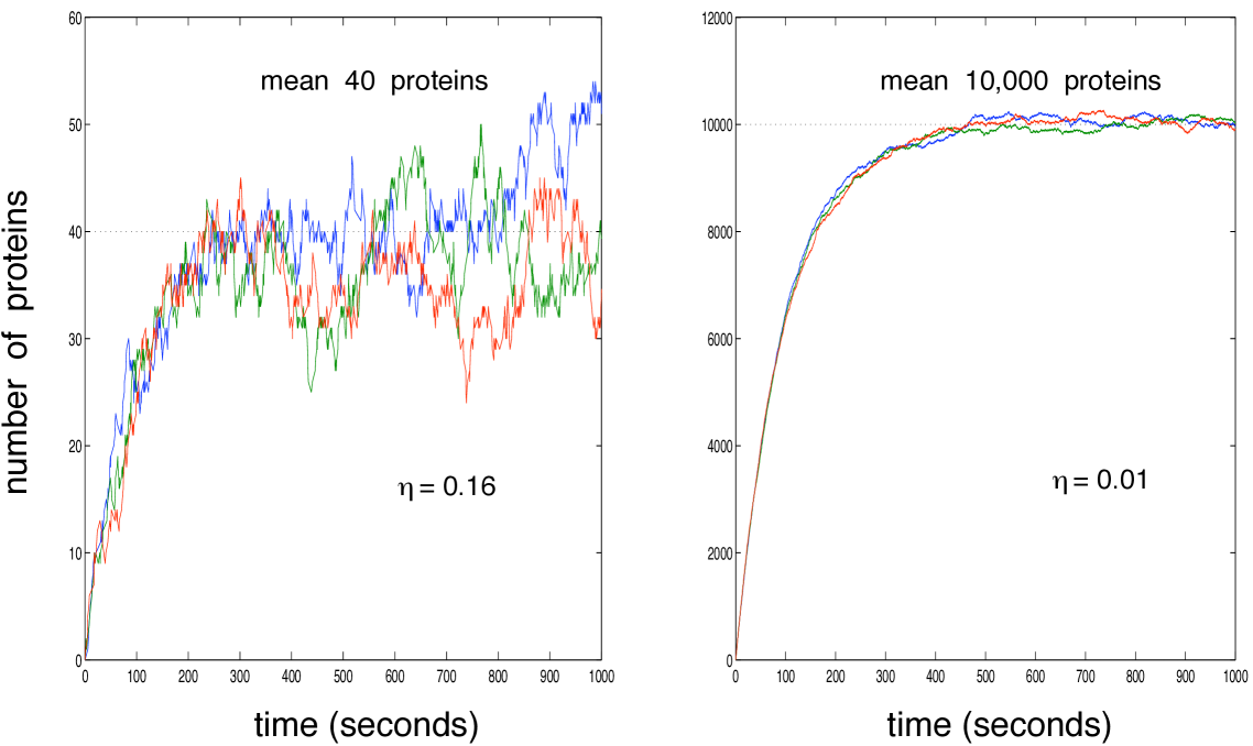
Figure 1: Three simulation runs of two birth-and-death models of gene expression (Eq. 13). Each model has different rate constants leading to different mean protein levels.

Recovering the deterministic equations

Solving the master equation is possible for linear systems, i.e. those with only first-order chemical reactions, but often only at steady-state [12, 21]. Solving for the moments of a master equation is often easier.

For the non-linear system of Eq. 6, we will use the master equation, (11), to derive the equation of motion for the mean of $C$. The mean of $C$ is defined as

$$\langle C(t)\rangle=\sum_{n_{A},n_{B},n_{C}}n_{C}P_{n_{A},n_{B},n_{C}}(t)$$ (30)

and is a function of time.

Multiplying (11) by $n_{C}$ and summing over $n_{A}$, $n_{B}$, and $n_{C}$ gives

$$\frac{\partial}{\partial t}\langle C\rangle = f\sum(n_{C}-1+1)(n_{A}+1)(n_{B}+1)P_{n_{A}+1,n_{B}+1,n_{C}-1}$$ (31)

$$-f\sum n_{A}n_{B}n_{C}P_{n_{A},n_{B},n_{C}}-d\sum n_{C}^{2}P_{n_{A},n_{B},n_{C}}$$

$$+d\sum(n_{C}+1-1)(n_{C}+1)P_{n_{A},n_{B},n_{C}+1}$$

where the terms in round brackets have been factored to follow the subscripts of $P$. Therefore, by using results such as

$$\langle ABC\rangle = \sum_{n_{A},n_{B},n_{C}=0}^{\infty}n_{A}n_{B}n_{C}P_{n_{A},n_{B},n_{C}}$$ (32)

$$= \sum_{n_{A},n_{B},n_{C}=0}^{\infty}(n_{A}+1)(n_{B}+1)(n_{C}-1)P_{n_{A}+1,n_{B}+1,n_{C}-1}$$

as $P_{n_{A},n_{B},n_{C}}(t)$ is zero if any of $n_{A}$, $n_{B}$, or $n_{C}$ are negative, we have

$$\frac{\partial}{\partial t}\langle C\rangle = f\Bigl{[}\langle ABC\rangle+\langle AB\rangle\Bigr{]}-f\langle ABC\rangle-d\langle C^{2}\rangle+d\Bigl{[}\langle C^{2}\rangle-\langle C\rangle\Bigr{]}$$ (33)

$$= f\langle AB\rangle-d\langle C\rangle$$

which is the microscope equation for the dynamics of the mean of $C$.

We can also consider the deterministic equation for the dynamics. Applying the law of mass action to this system, the concentration of $C$, $[C]$, obeys

$$\frac{d}{dt}[C]=\tilde{f}[A][B]-\tilde{d}[C]$$ (34)

where $\tilde{f}$ and $\tilde{d}$ are the macroscopic (deterministic) rate constants. The macroscopic concentration is related to the mean number of molecules by

$$[C]=\frac{\langle C\rangle}{V}$$ (35)

and so the deterministic equations are equations for the rate of change of the means of the different chemical species: using (35), (34) becomes

$$\frac{d}{dt}\langle C\rangle=\frac{\tilde{f}}{V}\langle A\rangle\langle B\rangle-\tilde{d}\langle C\rangle.$$ (36)

By comparing the deterministic equation, (36), with the microscopic equation, (33), we can relate the stochastic probabilities of reaction per unit time and the deterministic kinetic rates:

$$\tilde{f} = \frac{V\langle AB\rangle}{\langle A\rangle\langle B\rangle}\cdot f$$

$$\tilde{d} = d$$ (37)

For first-order reactions both the kinetic rate and the probability are the same. The macroscopic rate $\tilde{f}$ is usually measured under conditions where the deterministic approximation holds and numbers of molecules are large. We can write

$$\tilde{f} = \frac{V\Bigl{(}\langle A\rangle\langle B\rangle+\langle AB\rangle-\langle A\rangle\langle B\rangle\Bigr{)}}{\langle A\rangle\langle B\rangle}\cdot f$$ (38)

$$= Vf\cdot\left(1+\frac{\langle AB\rangle-\langle A\rangle\langle B\rangle}{\langle A\rangle\langle B\rangle}\right)$$

$$\simeq Vf$$

where the fluctuation term becomes negligible as the numbers of molecules increase because its numerator, the co-variance $\langle AB\rangle-\langle A\rangle\langle B\rangle$, is expected to be proportional to the mean number of molecules, while its denominator is proportional to the square of the mean number of molecules. Eq. (Example: A birth-and-death processes) is an explicit example of this statement. Eq. (38) is almost always used to relate the macroscopic rate and the probability of reaction for second-order reactions.

An exception: homo-dimerization reactions

A homo-dimerization reaction

$$\ce{A+A->[f]A_{2}}$$

occurs when two identical monomers combine to form a dimer. This reaction is common among transcription factors. The master equation is now

$$\frac{\partial P_{n_{A}}}{\partial t}=f\left[\left(\begin{array}[]{c}n_{A}+2\\ 2\end{array}\right)P_{n_{A}+2}-\left(\begin{array}[]{c}n_{A}\\ 2\end{array}\right)P_{n_{A}}\right]$$ (39)

where each coefficient is the number of ways of forming a dimer. Eq. (Recovering the deterministic equations) becomes

$$2\frac{\tilde{f}}{V}\langle A\rangle^{2}=f\langle A(A-1)\rangle.$$ (40)

Assuming that $\tilde{f}$ is measured for large numbers of molecules, we can write

$$\langle A(A-1)\rangle\simeq\langle A\rangle^{2}$$ (41)

and so to

$$\tilde{f}\simeq\frac{fV}{2}$$ (42)

which is the inter-conversion formula for dimerization reactions.

Simulating stochastic biochemical reactions

The Gillespie algorithm [16] is most commonly used to simulate intrinsic fluctuations in biochemical systems. The equivalent of two dice are rolled on the computer: one to choose which reaction will occur next and the other to choose when that reaction will occur. Assume that we have a system in which $n$ different reactions are possible, then the probability that starting from time $t$ a reaction only occurs between $t+\tau$ and $t+\tau+\delta\tau$ must be calculated for each reaction. Let this probability be $P_{i}(\tau)\delta\tau$ for reaction $i$, say.

For example, if reaction $i$ corresponds to the second-order reaction of Eq. 6, then

$${\cal P}(\mbox{reaction $i$ in time $\delta\tau$}) = n_{A}n_{B}f\delta\tau$$ (43)

$$= a_{i}\delta\tau$$

where $a_{i}$ is referred to as the propensity of reaction $i$. Therefore,

$$P_{i}(\tau)\delta\tau = {\cal P}(\mbox{no reaction for time $\tau$})$$ (44)

$$\times{\cal P}(\mbox{reaction $i$ happens in time $\delta\tau$})$$

$$\equiv P_{0}(\tau)a_{i}\delta\tau$$

with $P_{0}(\tau)$ the probability that no reaction occurs during the interval $\tau$. This probability is the product of the probability of having no reactions at time $\tau$ and the probability of no reactions occurring in time $\delta\tau$:

$$P_{0}(\tau+\delta\tau)=P_{0}(\tau)\Bigl{[}1-\sum_{j=1}^{n}a_{j}\delta\tau\Bigr{]}$$ (45)

which implies

$$\frac{dP_{0}}{d\tau}=-P_{0}\sum^{n}_{j=1}a_{j}$$ (46)

and so

$$P_{0}(\tau)=\exp\left(-\tau\sum a_{j}\right).$$ (47)

Thus we have

$$P_{i}(\tau)=a_{i}{\rm e}^{-\tau\sum a_{j}}$$ (48)

from (47).

To choose which reaction to simulate, an $n$-sided die is rolled with each side corresponding to a reaction and weighted by the reaction’s propensity. A second die is then used to determine the time when the reaction occurs by sampling from (47). All the chemical species and the time variable are updated to reflect the occurrence of the reaction, and the process is then repeated. See Gillespie (1977) [16] for more details.

Extrinsic fluctuations can be included by considering reaction rates that change with time [18]. A reaction rate is often a function of the concentration of another protein and so fluctuates because this protein concentration fluctuates. For example, $v_{0}$ in Fig. 2 is a function of the concentration of free RNA polymerases and $v_{1}$ is a function of the concentration of free ribosomes. By simulating extrinsic fluctuations with the desired properties before running the Gillepsie algorithm and then approximating this extrinsic time series by a sequence of linear changes over small time intervals, we can ‘feed’ the extrinsic fluctuations into the Gillepsie algorithm and so let a parameter, or many parameters, fluctuate extrinsically.

Langevin theory: an improved model of gene expression

Figure 2: A model of gene expression that explicitly includes transcription (rate $v_{0}$) and translation (rate $v_{1}$) as first-order processes. mRNA is denoted by $M$ and protein by $N$.

We can model transcription and translation as first-order reactions [22]. Both mRNA, $M$, and protein, $N$, are present, and each has their own half-life (determined by the inverse of their degradation rates).

The Langevin solution

Langevin theory gives an approximation to the solution of the master equation. It is strictly only valid when numbers of molecules are large. Stochastic terms are explicitly added to the deterministic equations of the system. For the model of Fig. 2, the deterministic equations are

$$\frac{dM}{dt} = v_{0}-d_{0}M$$

$$\frac{dN}{dt} = v_{1}M-d_{1}N.$$ (49)

A Langevin model adds a stochastic variable, $\xi(t)$, to each

$$\frac{dM}{dt} = v_{0}-d_{0}M+\xi_{1}(t)$$

$$\frac{dN}{dt} = v_{1}M-d_{1}N+\xi_{2}(t)$$ (50)

and is only fully specified when the probability distributions for the $\xi_{i}$ are given. The $\xi_{i}$ must be specified so that they mimic thermal fluctuations and model intrinsic fluctuations. The solution of the Langevin equation should then be a good approximation to that of the Master equation (and an exact solution in some limit).

To define $\xi$, we must give its mean and variance as functions of time and its autocorrelation.

Understanding stochasticity: autocorrelations

The autocorrelation time of a stochastic variable describes the average life-time of a typical fluctuation. We will denote it by $\tau$. Fig. 3 shows typical behaviour of a stochastic variable obeying a Poisson distribution. Time has been rescaled by the autocorrelation time. On average, the number of molecules changes significantly only over a time $\tau$ (1 in these units).

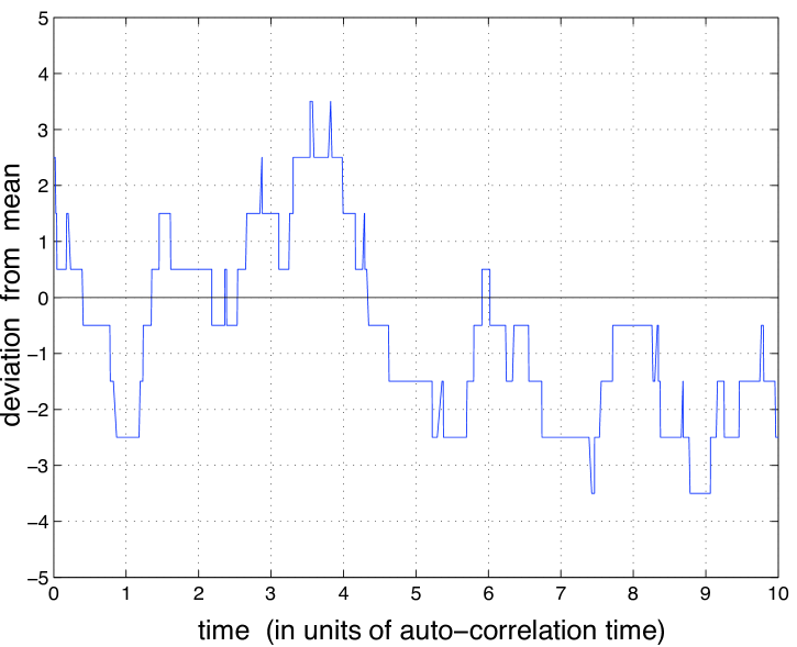
Figure 3: A time-series of a birth-death process. Time has been rescaled by the autocorrelation time. The deviation from the mean, $n-\langle n\rangle$, in numbers of molecules is plotted on the $y$-axis.

The autocorrelation time is found from the autocorrelation function. For a stochastic variable $N$, the autocorrelation function is

$$C_{N}(t_{1},t_{2}) = \left\langle\Bigl{[}N(t_{1})-\langle N(t_{1})\rangle\Bigr{]}\Bigl{[}N(t_{2})-\langle N(t_{2})\rangle\Bigr{]}\right\rangle$$ (51)

$$= \left\langle\Bigl{\{}N(t_{1})N(t_{2})-\langle N(t_{1})\rangle N(t_{2})-N(t_{1})\langle N(t_{2})\rangle+\langle N(t_{1})\rangle\langle N(t_{2})\rangle\Bigr{\}}\right\rangle$$

$$= \langle N(t_{1})N(t_{2})\rangle-\langle N(t_{1})\rangle\langle N(t_{2})\rangle.$$

It quantifies how a deviation of $N$ away from its mean at time $t_{1}$ is correlated with the deviation from the mean at a later time $t_{2}$. It is determined by the typical life-time of a fluctuation. When $t_{1}=t_{2}$, (51) is just the variance of $N(t)$.

Stationary processes are processes that are invariant under time translations and so are statistically identical at all time points. For a stationary process, such as the steady-state behaviour of a chemical system, the autocorrelation function obeys

$$C_{N}(t_{1},t_{2})=C_{N}(t_{2}-t_{1}).$$ (52)

It is a function of one variable: the time difference between the two time points considered. Fig. 4 shows the steady-state autocorrelation function for the Poisson model of gene expression. It is normalized by the variance and is fit well by an exponential decay: ${\rm e}^{-t/\tau}$. A typical fluctuation only persists for the timescale $\tau$ as enough new reaction events occur during $\tau$ to significantly change the dynamics and remove any memory the system may have had of earlier behaviour.

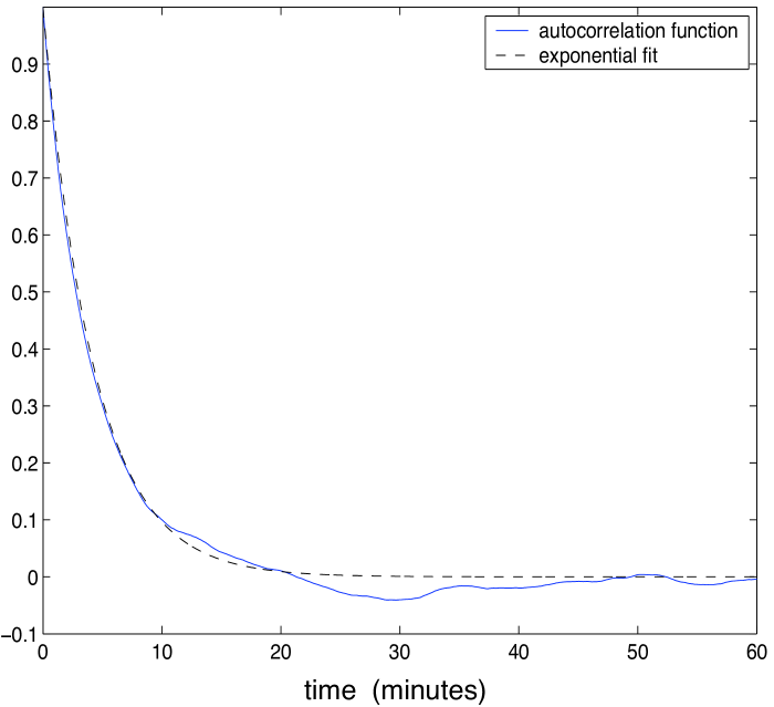
Figure 4: Auto-correlation function for a birth-death process. The dotted line is an exponential fit using an autocorrelation time of $1/d\simeq 4.2\;{\rm minutes}$.

For linear systems, the time-scale associated with degradation determines the steady-state autocorrelation time. Degradation provides the restoring force that keeps the number of proteins fluctuating around their mean steady-state value. The probability of degradation in time $\delta t$, $d\times n\times\delta t$, changes as the number of proteins $n$ changes. It increases as the number of proteins rises above the mean value, increasing the probability of degradation and of return to mean levels; it decreases as the number of proteins falls below mean levels, decreasing the probability of degradation and increasing again the probability of returning to mean values. For a linear system with multiple time-scales, the autocorrelation function is a sum of terms, each exponentially decreasing with $t_{1}-t_{2}$ at a time-scale set by the inverse of a degradation-like rate.

White noise

In Langevin theory, a stochastic variable, $\xi$, is added to each deterministic equation. This variable describes thermal fluctuations: those fluctuations that arise from collisions of the molecule of interest with surrounding molecules. Such collisions act to either increase or decrease the probability of reaction. A priori, there is no reason why thermal fluctuations would favour one effect over the other and so $\xi(t)$ is defined to have a mean of zero:

$$\langle\xi(t)\rangle=0.$$ (53)

The time-scale associated with collisions is assumed to be much shorter than the time-scale of a typical reaction. The changes in internal energy and position of the molecule of interest because of collisions with solvent molecules are therefore uncorrelated at the reaction time-scale. Mathematically, the autocorrelation time, $\tau$, of the autocorrelation function

$$C_{\xi}(t_{2}-t_{1})=\langle\xi(t_{1})\xi(t_{2})\rangle$$ (54)

is taken to zero. If $\Gamma/\tau$ is the variance of $\xi$ at time $t$, the auto-correlation function is

$$C_{\xi}(t_{2}-t_{1})=\frac{\Gamma}{\tau}{\rm e}^{-(t_{2}-t_{1})/\tau}$$ (55)

which becomes

$$\langle\xi(t_{1})\xi(t_{2})\rangle=\Gamma\delta(t_{2}-t_{1})$$ (56)

in the limit of $\tau\rightarrow 0$ where $\delta(t)$ is the Dirac delta function. A stochastic variable that obeys (53) and (56) is referred to as ‘white’. It is completely uncorrelated in time and has zero mean. Stochastic variables with zero mean and a finite auto-correlation time are considered ‘coloured’. The parameter $\Gamma$ determines the magnitude of fluctuations and needs to be carefully specified (see [12] for a discussion of how Einstein famously chose $\Gamma$ to appropriately model Brownian motion).

Langevin theory for stochastic gene expression

We now return to modelling the gene expression of Fig. 2. Eq. (The Langevin solution) is shown again below

$$\frac{dM}{dt} = v_{0}-d_{0}M+\xi_{1}(t)$$

$$\frac{dN}{dt} = v_{1}M-d_{1}N+\xi_{2}(t)$$ (57)

and is the deterministic equations of Fig. 2 with additive, white stochastic variables.

Although we expect $\xi_{1}$ and $\xi_{2}$ to have zero mean and zero autocorrelation times, we can show that this assumptions are true explicitly by first considering the steady-state solution of (Langevin theory for stochastic gene expression) in the absence of the stochastic variables $\xi_{i}$:

$$M_{s}=\frac{v_{0}}{d_{0}} N_{s}=\frac{v_{1}}{d_{1}}M_{s}$$ ; (58)

If we assume that the system is at or very close to steady-state, and consider a time interval $\delta t$ small enough such that at most only one reaction can occur, then $\xi_{1}$ and $\xi_{2}$ can only have the values

$$\xi_{i}\delta t=\left\{\begin{array}[]{l}+1\\ 0\\ -1\end{array}\right.$$ (59)

where $i=1$ or 2, as the number of $N$ or $M$ molecules can only increase or decrease by one or remain unchanged in time $\delta t$.

Define

$$P(i,j)={\cal P}(\xi_{1}\delta t=i,\xi_{2}\delta t=j)$$

i.e. the probability that the number of mRNAs changes by an amount $i$ and that the number of proteins changes by an amount $j$. Then the reaction scheme of Fig. 2 implies

$$P(+1,0) = v_{0}\delta t$$

$$P(+1,-1) = 0$$

$$P(+1,+1) = 0$$

$$P(-1,0) = d_{0}M_{s}\delta t$$

$$P(-1,+1) = 0$$

$$P(-1,-1) = 0$$

$$P(0,+1) = v_{1}M_{s}\delta t$$

$$P(0,0) = 1-v_{0}\delta t-v_{1}M_{s}\delta t-d_{0}M_{s}\delta t-d_{1}N_{s}\delta t$$

$$P(0,-1) = d_{1}N_{s}\delta t$$ (60)

at steady-state.

We can use these probabilities to calculate the moments of the $\xi_{i}$. First,

$$\langle\xi_{1}\delta t\rangle = (+1)\times v_{0}\delta t+(-1)\times d_{0}M_{s}\delta t+(0)\times(1-v_{0}\delta t-d_{0}M_{s}\delta t)$$ (61)

$$= (v_{0}-d_{0}M_{s})\delta t$$

$$= 0$$

and

$$\langle\xi_{2}\delta t\rangle = (+1)\times v_{1}M_{s}\delta t+(-1)\times d_{1}N_{s}\delta t$$ (62)

$$= (v_{1}M_{s}-d_{1}N_{s})\delta t$$

$$= 0$$

using (58). The means are both zero, as expected, and the $\xi_{i}$ act to keep the system at steady-state (as they should).

For the mean square, we have

$$\langle\xi_{1}^{2}\delta t^{2}\rangle = (+1)^{2}\times v_{0}\delta t+(-1)^{2}\times d_{0}M_{s}\delta t$$ (63)

$$= (v_{0}+d_{0}M_{s})\delta t$$

$$= 2d_{0}M_{s}\delta t$$

or

$$\langle\xi_{1}^{2}\rangle=\frac{2d_{0}M_{s}}{\delta t}$$ (64)

and, similarly,

$$\langle\xi_{2}^{2}\rangle = \frac{2d_{1}N_{s}}{\delta t}$$

$$\langle\xi_{1}\xi_{2}\rangle = 0$$ (65)

If the system is close to steady-state and the steady-state values of $M_{s}$ and $N_{s}$ are large enough such that

$$|M-M_{s}|\ll M_{s} |N-N_{s}|\ll N_{s}$$ ; (66)

then we can assume that (Langevin theory for stochastic gene expression) is valid for all times. Consequently, $\xi_{1}$ at time $t_{2}$, say, is completely uncorrelated with $\xi_{1}$ at time $t_{1}$, where $|t_{2}-t_{1}|>\delta t$ (just as the throws of a die whose outcomes are also given by fixed probabilities and are uncorrelated). Thus, we define as white stochastic terms

$$\langle\xi_{1}(t_{1})\xi_{1}(t_{2})\rangle = 2d_{0}M_{s}\delta(t_{2}-t_{1})$$

$$\langle\xi_{2}(t_{1})\xi_{2}(t_{2})\rangle = 2d_{1}N_{s}\delta(t_{2}-t_{1})$$

$$\langle\xi_{1}(t_{1})\xi_{2}(t_{2})\rangle = 0$$ (67)

with their magnitudes coming from (63) and (Langevin theory for stochastic gene expression).

This definition of $\xi_{1}$ and $\xi_{2}$ implies that the steady-state solution of (Langevin theory for stochastic gene expression) will have the true mean and variance of $N$ and $M$ obtained from the master equation, providing (66) is obeyed.

A further simplification

Although it is possible to directly solve the two coupled differential equations of (Langevin theory for stochastic gene expression), we can also take advantage of the different time-scales associated with mRNA and protein. Typically, mRNA life-time is of order minutes while protein life-time is of order hours in bacteria. Fig. 5 shows a simulated time series of protein and mRNA: protein has a longer autocorrelation time of $1/d_{1}$ compared to the mRNA autocorrelation time of $1/d_{0}$.

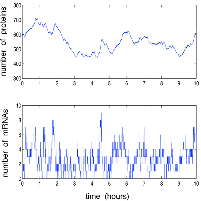
Figure 5: Protein and mRNA numbers from a simulation of the scheme of Fig. 2. Protein half-life is approximately 1 hour while that of mRNA is only 3 minutes.

Many mRNA fluctuations occur during one protein fluctuation, and so the mean level of mRNA reaches steady-state relatively quickly. Therefore, we can set

$$\frac{dM}{dt}\simeq 0$$ (68)

which implies that

$$M = \frac{v_{0}}{d_{0}}+\frac{\xi_{1}}{d_{0}}$$ (69)

$$= M_{s}+\frac{\xi_{1}}{d_{0}}$$

Consequently, the equation for protein, (Langevin theory for stochastic gene expression), becomes

$$\frac{dN}{dt}=v_{1}M_{s}-d_{1}N+\frac{v_{1}}{d_{0}}\xi_{1}+\xi_{2}$$ (70)

and so is a function of the two stochastic variables $\xi_{1}$ and $\xi_{2}$. To simplify (70), we define a new stochastic variable

$$\Psi=\frac{v_{1}}{d_{0}}\xi_{1}+\xi_{2}$$ (71)

which has mean

$$\langle\Psi\rangle=\frac{v_{1}}{d_{0}}\langle\xi_{1}\rangle+\langle\xi_{2}\rangle=0$$ (72)

from (61) and (62), and mean square

$$\langle\Psi(t_{1})\Psi(t_{2})\rangle = \left(\frac{v_{1}}{d_{0}}\right)^{2}\langle\xi_{1}(t_{1})\xi_{1}(t_{2})\rangle+2\left(\frac{v_{1}}{d_{0}}\right)\langle\xi_{1}(t_{1})\xi_{2}(t_{2})\rangle$$ (73)

$$+\langle\xi_{2}(t_{1})\xi_{2}(t_{2})\rangle$$

From Eqs. (Langevin theory for stochastic gene expression), this result simplifies

$$\langle\Psi(t_{1})\Psi(t_{2})\rangle = \left(\frac{v_{1}}{d_{0}}\right)^{2}2d_{0}M_{s}\delta(t_{2}-t_{1})+2d_{1}N_{s}\delta(t_{2}-t_{1})$$ (74)

$$= 2\left[\frac{v_{1}^{2}}{d_{0}}M_{s}+d_{1}N_{s}\right]\delta(t_{2}-t_{1})$$

$$= 2d_{1}\left[\frac{v_{1}}{d_{1}}M_{s}\frac{v_{1}}{d_{0}}+N_{s}\right]\delta(t_{2}-t_{1})$$

$$= 2d_{1}N_{s}\left[1+\frac{v_{1}}{d_{0}}\right]\delta(t_{2}-t_{1})$$

and so we need only consider one equation:

$$\frac{dN}{dt}=v_{1}M_{s}-d_{1}N+\Psi(t)$$ (75)

The effects of the mRNA fluctuations have been absorbed into the protein fluctuations and their magnitude has increased: compare (Langevin theory for stochastic gene expression) and (74).

Solving the model

Eq. (75) can be written as

$$\frac{d}{dt}\left(N{\rm e}^{d_{1}t}\right)=v_{1}M_{s}{\rm e}^{d_{1}t}+\Psi{\rm e}^{d_{1}t}$$ (76)

and so integrated

$$N(t){\rm e}^{d_{1}t}-N_{s}=\frac{v_{1}M_{s}}{d_{1}}\left({\rm e}^{d_{1}t}-1\right)+\int_{0}^{t}\Psi(t^{\prime}){\rm e}^{d_{1}t^{\prime}}dt^{\prime}$$ (77)

where we have assumed that $N=N_{s}$ when $t=0$. Thus

$$N(t)=N_{s}+{\rm e}^{-d_{1}t}\int_{0}^{t}\Psi(t^{\prime}){\rm e}^{d_{1}t^{\prime}}dt^{\prime}$$ (78)

Using the properties of $\Psi(t)$, (72) and (74), as well as (78), the mean protein number satisfies

$$\langle N(t)\rangle = N_{s}+{\rm e}^{-d_{1}t}\int_{0}^{t}\langle\Psi(t^{\prime})\rangle{\rm e}^{d_{1}t^{\prime}}dt^{\prime}$$ (79)

$$= N_{s}$$

and so the steady-state is stable to fluctuations (as expected).

We can also use (78) to find the autocorrelation function of the protein number:

$$\langle N(t_{1})N(t_{2})\rangle$$ (80)

$$=\biggl{\langle}\left[N_{s}+{\rm e}^{-d_{1}t_{1}}\int_{0}^{t_{1}}\Psi(t^{\prime}){\rm e}^{d_{1}t^{\prime}}dt^{\prime}\right]\times\left[N_{s}+{\rm e}^{-d_{1}t_{2}}\int_{0}^{t_{2}}\Psi(t^{\prime\prime}){\rm e}^{d_{1}t^{\prime\prime}}dt^{\prime\prime}\right]\biggr{\rangle}$$

$$=N_{s}^{2}+{\rm e}^{-d_{1}(t_{1}+t_{2})}\int_{0}^{t_{1}}{\rm e}^{d_{1}t^{\prime}}dt^{\prime}\int_{0}^{t_{2}}{\rm e}^{d_{1}t^{\prime\prime}}dt^{\prime\prime}\langle\Psi(t^{\prime})\Psi(t^{\prime\prime})\rangle$$

as $\langle\Psi\rangle=0$. From (74), we then have

$$\langle N(t_{1})N(t_{2})\rangle-N_{s}^{2}=2d_{1}N_{s}\left(1+\frac{v_{1}}{d_{0}}\right){\rm e}^{-d_{1}(t_{1}+t_{2})}\int_{0}^{t_{1}}dt^{\prime}\int_{0}^{t_{2}}dt^{\prime\prime}{\rm e}^{d_{1}(t^{\prime}+t^{\prime\prime})}\delta(t^{\prime}-t^{\prime\prime})$$ (81)

To evaluate the double integral, we need to determine when $t^{\prime}$ is equal to $t^{\prime\prime}$. If $t_{2}\geq t_{1}$, then the integral can be decomposed into

$$\int_{0}^{t_{2}}dt^{\prime}\int_{0}^{t_{1}}dt^{\prime\prime} = \left(\int_{t_{1}}^{t_{2}}dt^{\prime}+\int_{0}^{t_{1}}dt^{\prime}\right)\int_{0}^{t_{1}}dt^{\prime\prime}$$ (82)

$$= \int_{t_{1}}^{t_{2}}dt^{\prime}\int_{0}^{t_{1}}dt^{\prime\prime}+\int_{0}^{t_{1}}dt^{\prime}\int_{0}^{t_{1}}dt^{\prime\prime}$$

where we now explicitly see that $t^{\prime}>t^{\prime\prime}$ for the first term (and there will be no contribution from the delta function) and $t^{\prime}$ can equal $t^{\prime\prime}$ for the second term (and there will be a contribution from the delta function). Therefore,

$$\int_{0}^{t_{2}}dt^{\prime}\int_{0}^{t_{1}}dt^{\prime\prime}{\rm e}^{d_{1}(t^{\prime}+t^{\prime\prime})}\delta(t^{\prime}-t^{\prime\prime})$$ (83)

$$=\int_{t_{1}}^{t_{2}}dt^{\prime}\int_{0}^{t_{1}}dt^{\prime\prime}{\rm e}^{d_{1}(t^{\prime}+t^{\prime\prime})}\delta(t^{\prime}-t^{\prime\prime})+\int_{0}^{t_{1}}dt^{\prime}\int_{0}^{t_{1}}dt^{\prime\prime}{\rm e}^{d_{1}(t^{\prime}+t^{\prime\prime})}\delta(t^{\prime}-t^{\prime\prime})$$

$$=\int_{0}^{t_{1}}{\rm e}^{2d_{1}t^{\prime}}dt^{\prime}$$

$$=\frac{1}{2d_{1}}\left({\rm e}^{2d_{1}t_{1}}-1\right)$$

because the first integral evaluates to zero.

Consequently, (81) becomes

$$\langle N(t_{1})N(t_{2})\rangle-N_{s}^{2} = 2d_{1}N_{s}\left(1+\frac{v_{1}}{d_{0}}\right){\rm e}^{-d_{1}(t_{1}+t_{2})}\frac{1}{2d_{1}}\left({\rm e}^{2d_{1}t_{1}}-1\right)$$ (84)

$$= N_{s}\left(1+\frac{v_{1}}{d_{0}}\right)\left({\rm e}^{-d_{1}(t_{2}-t_{1})}-{\rm e}^{-d_{1}(t_{1}+t_{2})}\right)$$

and we finally have

$$\langle N(t_{1})N(t_{2})\rangle-\langle N(t_{1})\rangle\langle N(t_{2})\rangle=N_{s}\left(1+\frac{v_{1}}{d_{0}}\right)\left({\rm e}^{-d_{1}(t_{2}-t_{1})}-{\rm e}^{-d_{1}(t_{1}+t_{2})}\right)$$ (85)

as $\langle N(t)\rangle=N_{s}$. Eq. (85) is the autocorrelation function for protein number and becomes

$$C_{N}=N_{s}\left(1+\frac{v_{1}}{d_{0}}\right){\rm e}^{-d_{1}(t_{2}-t_{1})}$$ (86)

after long times $t_{2}>t_{1}\gg 1$. The protein autocorrelation time is $1/d_{1}$.

We can also find similar expressions for mRNA. Eq. (75) has the same structure as the equation for mRNA

$$\frac{dM}{dt}=v_{0}-d_{0}M+\xi_{1}(t)$$ (87)

with a constant rate of production and first-order degradation. The solution of (87) will therefore be of the same form as (86), but with $d_{1}$ replaced by $d_{0}$ and the magnitude of the stochastic term coming from (Langevin theory for stochastic gene expression) rather than (74). This substitution gives

$$C_{M}=M_{s}{\rm e}^{-d_{0}(t_{2}-t_{1})}$$ (88)

so that the autocorrelation time of the mRNA is $1/d_{0}$.

We can calculate the noise in mRNA when $t_{1}=t_{2}$ because then the autocorrelation becomes the variance:

$$\eta^{2}_{M} = \frac{\langle M(t)^{2}\rangle-\langle M(t)\rangle^{2}}{\langle M(t)\rangle^{2}}$$ (89)

$$= \frac{M_{s}}{M_{s}^{2}}$$

$$= \frac{1}{\langle M\rangle}$$

Eqs. (88) and (89) are the solutions to any birth-and-death model and correspond to the expressions given in (Example: A birth-and-death processes) and (29).

The protein noise is a little more complicated. It satisfies

$$\eta^{2}_{N} = \frac{1}{N_{s}}+\frac{v_{1}}{d_{0}}\frac{1}{N_{s}}$$ (90)

$$= \frac{1}{N_{s}}+\frac{d_{1}}{d_{0}}\frac{1}{M_{s}}$$

$$= \frac{1}{\langle N\rangle}+\frac{d_{1}}{d_{0}}\frac{1}{\langle M\rangle}$$

which should be compared with (29) for a birth-death process. The mRNA acts as a fluctuating source of proteins and increases the noise above the Poisson value. Eq. (90) can be described as

$$(\mbox{protein noise})^{2}=(\mbox{Poisson noise})^{2}+\frac{\mbox{mRNA lifetime}}{\mbox{protein lifetime}}\times(\mbox{mRNA noise})^{2}$$ (91)

The Poisson noise is augmented by a time average of the mRNA noise. As the protein life-time increases compared to the mRNA life-time, each protein averages over more mRNA fluctuations and the overall protein noise decreases. Ultimately, $\eta_{N}$ approaches the Poisson result as $d_{1}/d_{0}\rightarrow 0$.

More generally, we should include active and inactive states of the promoter. With this extension, the model of gene expression appears valid for bacteria [23], yeast [9], slime moulds [24], and mammalian cells [25, 26]. Physically, the two states of the promoter could reflect changes in the structure of chromatin, the binding of transcription factors, or stalling of RNA polymerases during transcription.

Typical numbers for constitutive expression

Some typical numbers for constitutive (unregulated) expression in E. coli are

$$d_{1}=1/\mbox{hour} d_{0}=1/\mbox{3 minutes}$$ ;

$$\langle N\rangle=10^{3} \langle M\rangle=5$$ ; (92)

and so (90) becomes

$$\eta^{2}_{N} = 1/1000+3/60\times 1/5$$ (93)

$$= 0.001+0.01$$

The mRNA term determines the overall magnitude of the noise.

Appendix 1: Dirac delta function

The Dirac delta function can be considered the limit of a zero mean normal distribution as its standard deviation tends to zero:

$$\delta(x)=\stackrel{{\scriptstyle\rm lim}}{{\scriptstyle n\rightarrow\infty}}\frac{n}{\sqrt{\pi}}{\rm e}^{-n^{2}x^{2}}$$ (A1)

This limit gives a function whose integral over all $x$ is one, but that becomes increasingly more and more spiked at zero (Fig. 6). Ultimately

$$\delta(x)=0\mbox{ for all $x\neq 0$}$$ (A2)

and is not strictly defined at $x=0$, but does retain the property

$$\int_{-\infty}^{\infty}\delta(x)dx=1.$$ (A3)

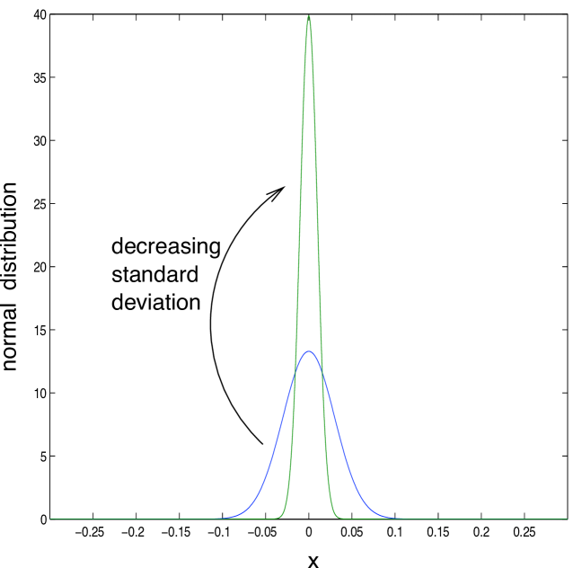
Figure 6: The Dirac delta function is the ‘spike’ limit of a normal distribution as its standard deviation tends to zero.

These two characteristics imply that the integral of a product of a delta function and another function, $f(x)$, will only give a non-zero result at $x=0$. The delta function effectively selects the value $f(0)$ from the integral:

$$\int_{-\infty}^{\infty}f(x)\delta(x)dx=f(0)$$ (A4)

or more generally

$$\int_{-\infty}^{\infty}f(x)\delta(x-y)dx=f(y).$$ (A5)

Appendix 2: Sampling from a probability distribution

Often we wish to sample from a particular probability distribution, $P(x)$, say. The cumulative distribution of $P(x)$ is

$$F(x)=\int_{x_{\rm min}}^{x}P(x^{\prime})dx^{\prime}$$ (A6)

and

$${\cal P}(x\leq x_{0}) = \int_{x_{\rm min}}^{x_{0}}P(x^{\prime})dx^{\prime}$$ (A7)

$$= F(x_{0})$$

A sketch of the typical behaviour of $F(x)$ is shown in Fig. 7. If $x\leq x_{0}$, then $F(x)\leq F(x_{0})$ because $F(x)$ is a monotonic increasing function (by definition).

Figure 7: A typical plot of cumulative frequency versus $x$.

To sample from $P(x)$, first let $y$ be a uniform random number with $0\leq y\leq 1$ (easily obtained on a computer), then

$${\cal P}(y\leq y_{0})=\int_{0}^{y_{0}}dy^{\prime}=y_{0}$$ (A8)

for some $0\leq y_{0}\leq 1$. Define

$$x=F^{-1}(y)$$ (A9)

where $F(x)$ is the cumulative frequency of $P(x)$. Consequently,

$${\cal P}(x\leq x_{0}) = {\cal P}(F^{-1}(y)\leq x_{0})$$ (A10)

$$= {\cal P}(F.F^{-1}(y)\leq F(x_{0}))$$

given that $F(x)$ is monotonic. As $F.F^{-1}(y)=y$, we have

$${\cal P}(x\leq x_{0}) = {\cal P}(y\leq F(x_{0}))$$ (A11)

$$= F(x_{0})$$

as $y$ is a sample between 0 and 1 from the uniform distribution: see (A8). Thus the $x$ of (A9) obeys (A7) and so is a sample from $P(x)$.

If we can calculate the inverse function of the cumulative frequency of a distribution $P(x)$, then applying this inverse function to a sample from the uniform distribution gives a sample from $P(x)$.

References

- [1] Kaern M, Elston TC, Blake WJ, Collins JJ (2005) Stochasticity in gene expression: from theories to phenotypes. Nat Rev Genet 6:451–464.
- [2] Shahrezaei V, Swain PS (2008) The stochastic nature of biochemical networks. Curr Opin Biotechnol 19:369–374.
- [3] Raj A, van Oudenaarden A (2008) Nature, nurture, or chance: stochastic gene expression and its consequences. Cell 135:216–226.
- [4] Eldar A, Elowitz MB (2010) Functional roles for noise in genetic circuits. Nature 467:167–173.
- [5] Elowitz MB, Levine AJ, Siggia ED, Swain PS (2002) Stochastic gene expression in a single cell. Science 297:1183–1186.
- [6] Swain PS, Elowitz MB, Siggia ED (2002) Intrinsic and extrinsic contributions to stochasticity in gene expression. Proc Natl Acad Sci USA 99:12795–12800.
- [7] Ozbudak EM, Thattai M, Kurtser I, Grossman AD, van Oudenaarden A (2002) Regulation of noise in the expression of a single gene. Nat Genet 31:69–73.
- [8] Blake WJ, Kaern M, Cantor CR, Collins JJ (2003) Noise in eukaryotic gene expression. Nature 422:633–637.
- [9] Raser JM, O’Shea EK (2004) Control of stochasticity in eukaryotic gene expression. Science 304:1811–1814.
- [10] Samoilov MS, Arkin AP (2006) Deviant effects in molecular reaction pathways. Nat Biotechnol 24:1235–1240.
- [11] Grima R (2010) An effective rate equation approach to reaction kinetics in small volumes: theory and application to biochemical reactions in nonequilibrium steady-state conditions. J Chem Phys 133:035101.
- [12] Van Kampen NG (1981) Stochastic processes in physics and chemistry (North-Holland, Amsterdam, The Netherlands).
- [13] Gillespie DT (2000) The chemical Langevin equation. J Chem Phys 113:297.
- [14] Hasty J, Pradines J, Dolnik M, Collins JJ (2000) Noise-based switches and amplifiers for gene expression. Proc Natl Acad Sci USA 97:2075–2080.
- [15] Swain PS (2004) Efficient attenuation of stochasticity in gene expression through post-transcriptional control. J Mol Biol 344:965–976.
- [16] Gillespie DT (1977) Exact stochastic simulation of coupled chemical reactions. J Phys Chem 81:2340–2361.
- [17] Paulsson J (2004) Summing up the noise in gene networks. Nature 427:415–418.
- [18] Shahrezaei V, Ollivier JF, Swain PS (2008) Colored extrinsic fluctuations and stochastic gene expression. Mol Syst Biol 4:196.
- [19] Friedman N, Cai L, Xie XS (2006) Linking stochastic dynamics to population distribution: an analytical framework of gene expression. Phys Rev Lett 97:168302.
- [20] Shahrezaei V, Swain PS (2008) Analytical distributions for stochastic gene expression. Proceedings of the National Academy of Sciences 105:17256–17261.
- [21] Gardiner CW (1990) Handbook of stochastic methods (Springer, Berlin, Germany).
- [22] Thattai M, van Oudenaarden A (2001) Intrinsic noise in gene regulatory networks. Proc Natl Acad Sci USA 98:8614–8619.
- [23] Golding I, Paulsson J, Zawilski SM, Cox EC (2005) Real-time kinetics of gene activity in individual bacteria. Cell 123:1025–1036.
- [24] Chubb JR, Trcek T, Shenoy SM, Singer RH (2006) Transcriptional pulsing of a developmental gene. Curr Biol 16:1018–1025.
- [25] Raj A, Peskin CS, Tranchina D, Vargas DY, Tyagi S (2006) Stochastic mRNA synthesis in mammalian cells. PLoS Biol 4:e309.
- [26] Sigal A, et al. (2006) Variability and memory of protein levels in human cells. Nature 444:643–646.