ABROA : Audio-Based Room-Occupancy Analysis using Gaussian Mixtures and Hidden Markov Models

Abstract

This paper outlines preliminary steps towards the development of an audio-based room-occupancy analysis model. Our approach borrows from speech recognition tradition and is based on Gaussian Mixtures and Hidden Markov Models. We analyse possible challenges encountered in the development of such a model, and offer several solutions including feature design and prediction strategies. We provide results obtained from experiments with audio data from a retail store in Palo Alto, California. Model assessment is done via leave-two-out Bootstrap and model convergence achieves good accuracy, thus representing a contribution to multimodal people counting algorithms.

1 INTRODUCTION

Information about the occupancy of a certain location is relevant for several applications, specially in surveillance tasks and staff management. For example, occupancy can be used to detect intruders in a house, or to generate optimal employee schedules according to shopper traffic. The existing systems for occupancy detection rely on multimodal systems, including video, Wifi, Bluetooth and, to a much lesser extent, audio. Conversely, the use of audio in occupancy estimation empowers the development of a model, not dependent on speaker separation, that is robust to issues that are common in computer vision and systems that rely on tracking electronic devices, such as occlusion and people clusters[1].

1.1 Related work

The occupancy estimation literature can be subdivided in invasive and non-invasive strategies. Invasive strategies [2, 3, 4] use various devices, e.g. smartphones and ultrasonic transmitters, to project sound, e.g. sinusoids and chirps, onto the environment and use the environment’s response to the projected sound to estimate activity in the space; Non-invasive strategies [5, 6, 7] rely on detecting speech sounds in the environment to estimate occupancy. In addition to potentially disturbing humans and animals, invasive strategies require the expensive task of deploying devices, e.g. 891 mobile devices to cover 600 square meters and less than 20 people [6], in the location and badly suffer from the addition of non-human objects and subjects to the space being analyzed. Non-invasive strategies that rely on speech only to estimate occupancy will disregard people who are in a space but not talking, and badly suffer from situations in which speech diarization is not possible. In addition, most of these systems are only able to handle small groups of people.

The limitations presented above and the lack of a standard technique or key paper on the topic of audio-based room-occupancy analysis confirm the need for the development of such a technique. There is no annotated dataset for audio-based room-occupancy analysis and, therefore, the acquisition of data remains a blatant challenge. Although [8] describes the layout of a rather promising prototype to estimate the occupancy of rooms and buildings based on audio, they provide no information on experiments nor results describing the efficiency of their system. In this paper we describe a system that is not invasive, suited for large groups of people, based on real data and computationally inexpensive.

2 METHODOLOGY

2.1 Dataset and ground truth

The dataset used in this research is comprised of proprietary audio recordings made with a smartphone placed in a retail store located in the United States. The smartphone’s microphone was aimed towards the inside of the store and placed at the store’s main and single entrance, at approximately 5 meters from the floor. The recordings took place during open hours (10h, 22h). The ground truth data is divided into 15-minute slices and it provides the cumulative occupancy at the end of each 15-minute time window. The ground truth was obtained from video data submitted to Amazon’s Mechanical Turk. Figure 2 illustrates the occupancy for that specific week. We invite the reader to consider the distribution of occupancy.

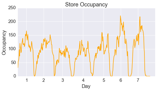
Figure 1: Occupancy

Figure 2: Store occupancy for the first week of April.

2.2 Room-occupancy Analysis

Several challenges are present in the development of an audio-based room-occupancy analysis system. In our context, the ground truth only provides information about the aggregated occupancy at the end of each 15-minute interval. This provides a challenge to feature selection, that is, selecting the audio slice that best represents the ground truth. In addition, since there’s one dependent variable for each 15-minute interval, regression models would require the design of summary statistics of the audio data to be used as the independent variable, thus extremely reducing the amount of information retrieved from each training sample. During evaluation we considered generalized linear models (GLM). Surprisingle, the mean error of the best linear model, Poisson Regression, was 33% worse than the GMM-HMM model described in this paper.

2.2.1 Audio Features

In our experiments we performed cross-validation on the training set using lasso regression models with the following features and linear regression models using all posible combination of the following features:

amplitude

median, mean, standard deviation

spectral

centroid, spread, skewness, kurtosis, slope

mfcc

raw, 1st delta, 2nd delta

We observed the p-values, 5% significance, of the regression models and concluded that the MFCC features contributed the most to prediction accuracy on the training set. Given this conclusion, our room-occupancy analysis algorithm uses the well-known Mel-Frequency Cepstral Coefficients[9] (MFCC). A total of 20 MFCCs (computed with a FFT Size of 4096 samples, Hop Size of 1024 samples and audio sample rate is 11050 hz) along with their first (20 features) and second (20 features) deltas[10] assembling a feature vector with 60 dimensions total. Given that sounds produced by humans are rarely stationary, the delta features provide valuable information.

2.2.2 Window selection

Our labeled data provides the cumulative occupancy at the end of a 15-minute time window. This represents two challenges: first, it is necessary to find out what temporal slice of the audio data should be used; second, the length of this slice must be chosen such that it maximizes the model’s performance. Window size is chosen under the one-standard-error rule using 50 iterations of leave-two-out Bootstrap with window sizes in the interval [30, 260] seconds, with a 10 seconds step size and starting at the end and increasing towards the beginning of the audio file.

2.2.3 GMM-HMM model

We propose a solution that references the speech recognition literature[11] and combines Gaussian Mixtures with Hidden Markov Models. The GMM is appropriate, for it provides a better categorization of the distribution of the audio features and a reliable estimate of the likelihood function, $p(X|\lambda)$, where $X={x_{1},x_{2},\ldots,x_{T}}$ is a sequence of feature vectors (MFCCs and deltas in our case), $x_{t}$ is a feature vector indexed at discrete time $t\in[1,2,...,T]$, and $\lambda$ represents some model. As described in[12], for a D-dimensional feature vector $x$ (60-dimensional in our case), the mixture density used for the likelihood of data $x$ given model $\lambda$ is defined as:

$$p(x|\lambda)=\sum_{i=1}^{M}w_{i}p_{i}(x)$$ (1)

This density is a weighted linear combination of $M$ unimodal Gaussian densities, $p_{i}(x)$, with parameters $\mu_{i}$ ($D\times 1$ mean vector) and $\Sigma_{i}$ ($D\times D$ covariance matrix):

$$p_{i}(x)=\frac{1}{(2\pi)^{D/2}|\Sigma_{i}|^{1/2}}\exp\{-\frac{1}{2}(x-\mu_{i})^{\prime}\Sigma_{i}^{-1}(x-\mu_{i})\}$$ (2)

Under the assumptions in[12], our model only uses the diagonal covariance matrix and the maximum likelihood model parameters are estimated using the well-known iterative expectation-maximization (EM) algorithm[11]. Traditionally, the feature vectors of $X$ are assumed independent and the log-likelihood for some sequence of feature vectors X is computed as:

$$LL(X|\lambda)=\sum_{t=1}^{T}log(p(x_{t}|\lambda))$$ (3)

We bin our occupancy data by taking the integer square root of occupancy values, thus circumscribing the problem of creating one GMM per occupancy value. The lowest occupancy is 0 and the maximum is 221, thus producing 15 occupancy bins. For each occupancy bin and its respective audio data, one bin-dependent GMM is trained with the MFCC features described above and using the Bayesian Information Criterion (BIC) for model selection over the number of components in the set $C=\left\{2,3,4,5,6,7,8,16,32\right\}$ on a test set.

In addition to the GMM, a HMM[13] can be used to compute $P(O|\lambda)$, that is the probability of the observation sequence $O=o_{1},o_{2},\dots,o_{T}$, i.e. occupancy sequence, given model $\lambda$. As described in[14], the probability of observations $O$ for a fixed state sequence $Q=q_{1},q_{2},\dots,q_{T}$, $P(O|Q,\lambda)$ is:

$$\prod_{t=1}^{T}P(o_{t}|q_{t},\lambda)=b_{q_{1}}(o_{1})b_{q_{2}}(o_{2})...b_{q_{T}}(o_{T})$$ (4)

where $b$ is an array storing the emission probabilities at time $t$ given model (bin-dependent GMM in our case). The probability of the state sequence $Q$ is given by:

$$P(Q|\lambda)=\pi_{q_{1}}a_{q_{1}q_{2}}a_{q_{2}q_{3}}...a_{q_{T-1}q_{T}}$$ (5)

where $\pi$ is an array storing the initial probabilities and $a$ is an array storing the transition probability from state $q_{t}$ to state $q_{t+1}$. We can calculate the probability of the observations given the model as:

$$P(O|\lambda)=\sum_{Q}P(O|Q,\lambda)P(Q|\lambda)$$ (6)

Decoding of the hidden state is computed using the Viterbi[15] algorithm to find the best path (single best state sequence) for an observation sequence. We define the probability of the best state path for the partial observation sequence as:

$$\delta_{t}(i)=\max_{q_{1},q_{2},\cdots,q_{t-1}}P(q_{1}q_{2},\cdots,q_{t}=s_{1},o_{1},o_{2},\cdots,o_{t}|\lambda)$$ (7)

Figure 3 illustrates our system and its use of the Hidden Markov Model and the Viterbi algorithm. Each circle represents the log-likelihood score of each feature vector given each binned GMM. The lines represent the transition probabilities and the highlighted states and bold lines show the state path that maximizes the log-likelihood.

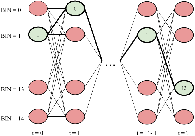
Figure 3: HMM and Viterbi illustration

3 EXPERIMENTS AND RESULTS

Several techniques were used for prediction, starting with using the log-likelihoods of each feature vector given each GMM and ending with a HMM.

3.1 Prediction with GMMs

Following the bin-dependent GMM training, two prediction strategies are chosen, including aggregating the posterior probabilities of each GMM and majority voting.

3.1.1 Posterior Probabilities Aggregation (PPA)

This procedure consists of aggregating the posterior probabilities of each state by computing the sum of bin occupancy predictions weighted by their posterior probabilities. Let $x$ be an audio feature vector and $\Lambda$ be a set of 15 bin-dependent GMMs. From Bayes theorem:

$$P(x|\Lambda_{i})=\frac{P(\Lambda_{i}|x)P(x)}{P(\Lambda_{i})}$$ (8)

Assuming that $P(\Lambda)$ is uniform and knowing that $P(x)$ is similar for all models, we conclude that $P(\Lambda_{i}|x)\propto P(x|\Lambda_{i})$. Finally, we define the estimated occupancy bin ($\hat{B}$) for feature vector $x$ at time $t$ and models $\Lambda$ as:

$$\hat{B}(x_{t})=\sum^{|\Lambda|-1}_{i=0}ie^{LL(x_{t}|\Lambda_{i})}$$ (9)

3.1.2 Majority Voting (MJ)

This procedure consist of calculating the log-likelihood, $LL(X,\lambda)$ of the audio features given each bin-dependent GMM and finally selecting the bin that more often has the highest log-likelihood score.

Using the GMM only approach and these techniques, informally speaking the prediction results circulate around the correct prediction value. However, the results for both techniques show jumps in occupancy prediction that are rather unlikely because the model ignores transition probabilities between states. Therefore, we decided to address this problem by using a HMM and the Viterbi algorithm.

3.2 Prediction with HMM and Viterbi

This strategy divides prediction into four stages, as described in Algorithm 1. The first computes the log-likelihood of the audio features given each bin-dependent GMM; the second applies the Viterbi algorithm to the computed log-likelihoods to obtain the best path for a specific time window. The third predicts the occupancy bin using posterior probabilities aggregation or majority voting; finally, the inverse of the square root of the predicted bin is calculated, thus translating the prediction back into the linear domain. For the HMM, the initial probabilities $\pi$ are uniform (1/15), the emission probabilities $b$ are computed using the GMMs and the transition probabilities $a$ are derived using heuristics.

Data: audio features

Result: predictions

GMMs $\leftarrow$ Train Bin-dependent GMMs on features

for feature in audio features do

       LLs $\leftarrow$ computeLL(feature, GMMs);

       bestpath $\leftarrow$ viterbi(LLs);

       prediction $\leftarrow$ PPAorMV(bestpath);

       predictions $\leftarrow$ [predictions, prediction²];

      

end for

Algorithm 1 Occupancy Prediction

3.3 Model Assessment and Selection

We used leave-two-out Bootstrap[16] for model assessment and selection, as it is a suitable technique for our small dataset of 386 samples. The Bootstrap technique was used to estimate the best window size, within the range [30, 260] seconds, and the most accurate prediction strategy based on the HMM-Viterbi model. For each window size and prediction strategy, a total of 50 bootstrap iterations were performed and the prediction errors were computed.

Figure 4 shows bootstrapped root mean squared errors (RMSE) for all window sizes and using the MJ and PPA techniques. Accuracy increases, specially in PPA, almost linearly and proportionally to the window size.

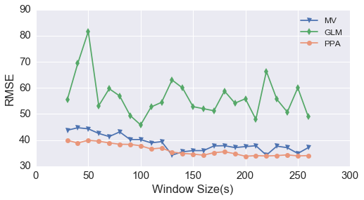
Figure 4: RMS errors for different windows and prediction techniques using HMM-Viterbi and Poisson Regression(GLM). The PPA technique converges around 210 seconds and considerably outperforms the MV and GLM techniques.

Model and window selection is performed using the one-standard-error rule and analysis of the violin plot provided in Figure 5. The best predictor uses the PPA technique with a window size of 210 seconds.

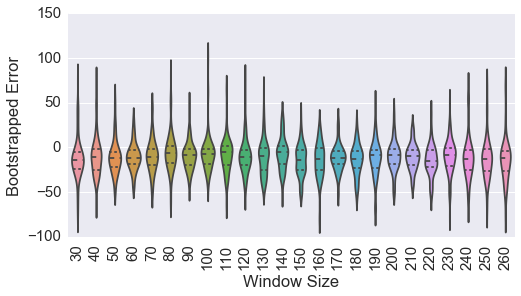
Figure 5: Bootstrapped error using GMM-HMM and PPA. Overall the bootstrapped error is below zero, thus suggesting that the model on average underpredicts.

Figure 6 shows room-occupancy predictions with a window of 210 seconds and both prediction techniques. Although the predictions made by both strategies closely follow the ground truth’s profile, there are individual large errors such as around sample indices 10 and 80.

4 CONCLUSION AND FUTURE WORK

We have described an algorithm for audio-based room-occupancy analysis that relies on Gaussian Mixtures and Hidden Markov Models. Our algorithm has advantages over other algorithms for audio-based occupancy analysis:

It is not invasive

our algorithm does not require projecting audio into an environment, thus not causing disturbance to humans or animals present.

It handles large groups

our algorithm is capable of handling occupancy prediction up to 200 people and this capacity can be extended given the appropriate training data.

It is inexpensive

prediction is computationally cheap and can be easily done on a smart phone, thus preventing privacy issues that might arise if audio data is sent over the network for prediction.

We analyzed different types of prediction techniques and concluded that the GMM-HMM posterior probabilities aggregation is the preferred approach, yielding better results than all other strategies explored. The algorithm performed considerably well in retail store environments with occupancy up to 200 people.

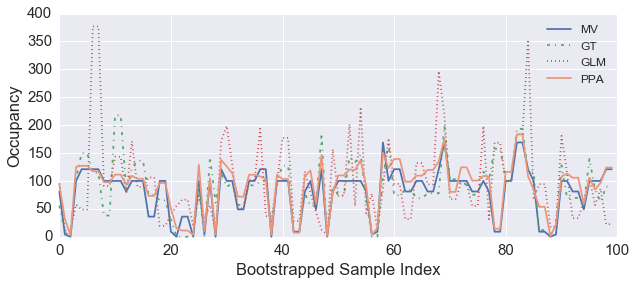
Figure 6: Ground Truth (GT) and predictions using the above described techniques (MV and PPA). The model performs well, in spite of two crass errors between indices 0 and 20. Unexpectedly, the generalized linear model (Poisson Regression) performs considerably worse then the models proposed in this paper.

The results from the current work validate the model and justify collecting more data to build a more balanced dataset with the foresight of increasing accuracy. In addition, we plan to use occupancy data to create the transition probabilities, instead of relying on ad-hoc rules. Last, we plan to add a Voice Activity Detection pre-processing step to the pipeline, denoise the audio data and perform comparative analysis with the results obtained in this paper.

References

- [1] T. B. Moeslund and E. Granum, “A survey of computer vision-based human motion capture,” Computer vision and image understanding, vol. 81, no. 3, pp. 231–268, 2001.
- [2] S. Srinivasan, A. Pandharipande, and D. Caicedo, “Presence detection using wideband audio-ultrasound sensor,” Electronics Letters, vol. 48, no. 25, pp. 1577–1578, 2012.
- [3] C. Xu, S. Li, G. Liu, Y. Zhang, E. Miluzzo, Y.-F. Chen, J. Li, and B. Firner, “Crowd++: unsupervised speaker count with smartphones,” in Proceedings of the 2013 ACM international joint conference on Pervasive and ubiquitous computing. ACM, 2013, pp. 43–52.
- [4] O. Shih and A. Rowe, “Occupancy estimation using ultrasonic chirps,” in Proceedings of the ACM/IEEE Sixth International Conference on Cyber-Physical Systems. ACM, 2015, pp. 149–158.
- [5] M. Khan, H. Hossain, and N. Roy, “Infrastructure-less occupancy detection and semantic localization in smart environments,” in Proceedings of the 12th international conference on mobile and ubiquitous systems: computing, networking and services, 2015.
- [6] P. G. Kannan, S. P. Venkatagiri, M. C. Chan, A. L. Ananda, and L.-S. Peh, “Low cost crowd counting using audio tones,” in Proceedings of the 10th ACM Conference on Embedded Network Sensor Systems. ACM, 2012, pp. 155–168.
- [7] S. Stillman and I. Essa, “Towards reliable multimodal sensing in aware environments,” in Proceedings of the 2001 workshop on Perceptive user interfaces. ACM, 2001, pp. 1–6.
- [8] S. Uziel, T. Elste, W. Kattanek, D. Hollosi, S. Gerlach, and S. Goetze, “Networked embedded acoustic processing system for smart building applications,” in Design and Architectures for Signal and Image Processing (DASIP), 2013 Conference on. IEEE, 2013, pp. 349–350.
- [9] B. Gold, N. Morgan, and D. Ellis, Speech and audio signal processing: processing and perception of speech and music. John Wiley & Sons, 2011.
- [10] S. Furui, “Speaker-independent isolated word recognition based on emphasized spectral dynamics,” in Acoustics, Speech, and Signal Processing, IEEE International Conference on ICASSP’86., vol. 11. IEEE, 1986, pp. 1991–1994.
- [11] L. Rabiner, “A tutorial on hidden markov models and selected applications in speech recognition,” Proceedings of the IEEE, vol. 77, no. 2, pp. 257–286, 1989.
- [12] D. A. Reynolds, T. F. Quatieri, and R. B. Dunn, “Speaker verification using adapted gaussian mixture models,” Digital signal processing, vol. 10, no. 1, pp. 19–41, 2000.
- [13] L. Rabiner and B.-H. Juang, “An introduction to hidden markov models,” ASSP Magazine, IEEE, vol. 3, no. 1, pp. 4–16, 1986.
- [14] P. Blunsom, “Hidden markov models,” Lecture notes, August, vol. 15, pp. 18–19, 2004.
- [15] G. D. Forney Jr, “The viterbi algorithm,” Proceedings of the IEEE, vol. 61, no. 3, pp. 268–278, 1973.
- [16] T. Hastie, R. Tibshirani, J. Friedman, T. Hastie, J. Friedman, and R. Tibshirani, The elements of statistical learning. Springer, 2009.