Entanglement as a resource for discrimination of classical environments

Abstract

We address extended systems interacting with classical fluctuating environments and analyze the use of quantum probes to discriminate local noise, described by independent fluctuating fields, from common noise, corresponding to the interaction with a common one. In particular, we consider a bipartite system made of two non interacting harmonic oscillators and assess discrimination strategies based on homodyne detection, comparing their performances with the ultimate bounds on the error probabilities of quantum-limited measurements. We analyze in details the use of Gaussian probes, with emphasis on experimentally friendly signals. Our results show that a joint measurement of the position-quadrature on the two oscillators outperforms any other homodyne-based scheme for any input Gaussian state.

I Introduction

The effects of the interaction of quantum systems with their environments have been widely studied in the last decades. In general, environment-induced decoherence wei01 ; bre01 is detrimental for the quantum features of a localized system: loss of nonclassicality har01 ; zur01 ; zur02 or disentanglement may arise asymptotically or after a finite interaction time ser1 ; ser2 ; ser23 ; ebe10 . On the other hand, extended systems experience more complex decoherence phenomena: the subparts of a system may interact with indepenent environments or, more interestingly, with a common one, corresponding to collective decoherence or dissipation, which may result in preservation of quantum coherence as well as preservation and creation of entanglement bra01 ; zha01 ; flo01 ; pra01 ; con01 ; paz01 or superradiance bro01 ; gro01 ; pal01 ; riv01 ; zan01 ; dua01 ; kwi01 ; dic01 .

Decoherence and dissipation into a common bath may arise spontaneously in some structured environments, but it may also be engineered bar01 ; ver01 to achieve specific goals. In both cases, the common decoherence mechanism may mingle or even being overthrown by local processes, leading to undesidered loss of quantum features. The discrimination between the presence of local or common environments is thus a relevant tool to fight decoherence and preserve quantum coherence.

Describing the interaction with an external environment in a full quantum picture may be challenging. On the other hand, in many situations the action of the environment on a quantum system may be represented as an external random force on the system itself. Such random forces are described in terms of classical stochastic fields (CSF)gar01 . As a matter of fact, the description of a quantum environment in terms of CSFs is often very accurate in capturing the quantum features of the dynamics. Besides, many system-environment interactions have a classical equivalent description hel01 ; hel02 ; cro01 ; wit01 ; str02 ; sto01 and there are situations where the environment can be effectively simulated classically tur01 . Finally, we mention that in several situations of experimental interest ast01 ; gal01 ; abe01 ; str01 quantum systems interact with inherently classical Gaussian noise.

In this framework, the main goal of this paper is to design a successful strategy to discriminate which kind of interaction, either local or common, occurs when an extended quantum probe interacts with a classical fluctuating environment. This is a channel discrimination problem, which we address upon considering a quantum probe interacting with either a local or a common bath, and then solving the corresponding state discrimination problem. In particular, in order to assess the role of entanglement with nearly analytic results, we consider a bipartite system made of two non interacting harmonic oscillators. The local noise scenario is described by the interaction of each oscillator with independent CSFs whereas common noise is described as the coupling between the two oscillators with the same CSF. The dynamics of this model has been analyzed recently tra01 revealing the existence of a rich phenomenology, which turns out to be a resource for discrimination purposes.

The lowest probability of error achievable in a quantum discrimination problem is known as Helstron bound hel03 . In several situations, such bound can be approximated by the Quantum Chernoff Bound (QCB) aud02 ; pir01 , originally derived in the setting of asymptotically many copies. Despite being less precise, the QCB turns out to be more versatile: it is easier to evaluate and can be used as distinguishability measure between qubits and single-mode Gaussian states cals01 ; aud01 , and for these reasons it constitutes a benchmark in quantum discrimination. On the other hand, the Helstrom bound may be challenging from the experimental point of view and a question arises about the performances achievable using feasbile measurements and realistic probe preparations.

In this paper, we analyze in details discrimination strategies based on homodyne detection, which has already proven to be useful in discrimination of quantum states witt01 or binary communication schemes oliv01 . Also, we analyze in details the performances of Gaussian states used as probe preparation, including many lab-friendly input signals.

Our results show that a joint measurement of the position on the two oscillators outperforms any other homodyne-based scheme, whatever input Gaussian state of the probe is employed. In terms of error probability, a discrimination scheme based on homodyne detection easily outperforms the QCB using (entangled) squeezed thermal states as input preparation.

The paper is organized as follows. In Sec. II we introduce the interaction model, we discuss the dynamics of the system in both local and common scenarios and describe the classes of Gaussian states we use later on in the paper. in Sec. III we introduce the necessary tools of discrimination theory. In Sec. IV we build step by step the discrimination strategy and check its performance with some lab-friendly Gaussian input states. Finally, in Sec, V, we optimize the discrimination strategy looking for the optimal Gaussian input state. Section VI then closes the paper with some concluding remarks.

II The Interaction Model

We consider two non-interacting harmonic quantum oscillators with natural frequencies $\omega_{1}$ and $\omega_{2}$ and describe the dynamics of this system in two different regimes: in the first one each oscillator is coupled to one of two independent non-interacting stochastic fields: this scenario is dubbed as local noise case. In the second regime, the oscillators are coupled to the same classical stochastic field, so we dub this case as common noise. In both case, the Hamiltonian $H$ is composed by a free and an interaction term. The free Hamiltonian $H_{0}$ is given by

$$H_{0} =\hbar\sum_{j=1}^{2}\omega_{j}a_{j}^{\dagger}a_{j}.$$ (1)

in both regimes, whereas the interaction term $H_{I}$ differs. In the following, we introduce the local and the common interaction Hamiltonians.

II.1 Local Interaction

The interaction Hamiltonian $H_{{\hbox{\tiny L}\,}}$ in the local model reads

$$H_{{\hbox{\tiny L}\,}}(t) =\sum_{j=1}^{2}a_{j}\bar{C_{j}}(t)e^{i\delta_{j}t}+a^{\dagger}_{j}C_{j}(t)e^{-i\delta_{j}t}$$ (2)

where the annihilation operators $a_{1},a_{2}$ represent the oscillators, each one coupled to a different local stochastic field $C_{j}(t)$ with $j=1,2$, and $\delta_{j}=\omega_{j}-\omega$ is the detuning between the carrier frequency of the field and the natural frequency of the $j$-th oscillator. Throughout the paper, we will consider the Hamiltonian rescaled in units of energy $\hbar\omega_{0}$ (for a reason to be pointed out later). Under this condition, the stochastic fields $C_{1}(t),C_{2}(t)$, their central frequency $\omega$, the interaction time $t$, and the detunings all become dimensionless quantities.

The presence of fluctuating stochastic fields leads to an explicitly time-dependent Hamiltonian, whose corresponding evolution operator is given by

$$U_{{\hbox{\tiny L}\,}}(t)={\cal T}\exp\left\{-i\int_{0}^{t}\!\!ds\,H_{{\hbox{\tiny L}\,}}(s)\right\}\,,$$ (3)

where ${\cal T}$ is the time ordering. The evolved density operator is formally given by

$$\rho_{{\hbox{\tiny L}\,}}(t)=U_{{\hbox{\tiny L}\,}}(t)\rho(0)U^{\dagger}_{{\hbox{\tiny L}\,}}(t).$$ (4)

The explicit form of the density operator can be found following the very same steps described in tra01 . The evolution of the density operator of the system then reads

$$\rho_{L}(t) =\left[D(\phi_{a},\phi_{b})\rho_{0}D^{\dagger}(\phi_{a},\phi_{b})\right]_{F}$$ (5)

where $D_{j}(\alpha)=\exp(\alpha a_{j}^{\dagger}-\alpha^{*}a_{j})$ is the displacement operator, $D(\alpha_{1},\alpha_{2})=D(\boldsymbol{\alpha})=D_{1}(\alpha_{1})D_{2}(\alpha_{2})$ and $\left[\ldots\right]_{F}$ is the average over the realizations of the stochastic fields.

In the local scenario, we assume each CSF

$$C_{j}(t)=C_{j}^{(x)}(t)+iC_{j}^{(y)}(t),$$

described as a Gaussian stochastic process with zero mean $[C_{j}^{(x)}(t)]_{F}=[C_{j}^{(y)}(t)]_{F}=0$ and autocorrelation matrix given by

$$\left[C_{j}^{(x)}(t_{1})C_{k}^{(x)}(t_{2})\right]_{F} =\left[C_{j}^{(y)}(t_{1})C_{k}^{(y)}(t_{2})\right]_{F}$$

$$=\delta_{jk}K(t_{1},t_{2})$$ (6)

$$\left[C_{j}^{(x)}(t_{1})C_{k}^{(y)}(t_{2})\right]_{F} =\left[C_{j}^{(y)}(t_{1})C_{k}^{(x)}(t_{2})\right]_{F}=0$$ (7)

where we introduced the kernel autocorrelation function $K(t_{1},t_{2})$. Upon performing the stochatic average, one finally recovers a Gaussian map describing the evolution of the state of the system under the assumption of local interaction

$$\rho_{{\hbox{\tiny L}\,}}(t)=\mathcal{G}_{{\hbox{\tiny L}\,}}[\rho(0)]=\int\frac{d^{4}\boldsymbol{\zeta}}{\pi^{2}}g_{{\hbox{\tiny L}\,}}(\boldsymbol{\zeta})D(\boldsymbol{\zeta})\rho(0)D^{\dagger}(\boldsymbol{\zeta})$$ (8)

where $g_{{\hbox{\tiny L}\,}}(\boldsymbol{\zeta})$ is the Gaussian function

$$g_{{\hbox{\tiny L}\,}}(\boldsymbol{\zeta})=\frac{\exp(-\frac{1}{2}\,\boldsymbol{\zeta}\cdot\boldsymbol{\Omega}\cdot\boldsymbol{\sigma}_{{\hbox{\tiny L}\,}}^{-1}\cdot\boldsymbol{\Omega}^{T}\cdot\boldsymbol{\zeta}^{T})}{\sqrt{\mbox{det}[\boldsymbol{\sigma}_{{\hbox{\tiny L}\,}}]}}$$ (9)

$\boldsymbol{\sigma}_{{\hbox{\tiny L}\,}}$ and the symplectic matrix $\boldsymbol{\Omega}$ being given by

$$\boldsymbol{\Omega}=\left(\begin{array}[]{cc}0&1\vspace{0.1 cm}\\ -1&0\end{array}\right)\quad\boldsymbol{\sigma}_{{\hbox{\tiny L}\,}}=\left(\begin{array}[]{cc}\beta_{1}(t)\mathbb{I}_{2}&0\vspace{0.1 cm}\\ 0&\beta_{2}(t)\mathbb{I}_{2}\end{array}\right).$$ (10)

The matrix $\boldsymbol{\sigma}_{{\hbox{\tiny L}\,}}$ is the covariance of the noise function $g_{{\hbox{\tiny L}\,}}(\boldsymbol{\sigma})$ and its matrix elements are given by

$$\beta_{j}(t,t_{0})=\int_{t_{0}}^{t}\int_{t_{0}}^{t}ds_{1}ds_{2}\cos[\delta_{j}(s_{1}-s_{2})]K(s_{1},s_{2}).$$ (11)

II.2 Common Interaction

The interaction Hamiltonian $H_{{\hbox{\tiny C}\,}}$ for the common noise case reads as follows

$$H_{{\hbox{\tiny C}\,}}(t) =\sum_{j=1}^{2}a_{j}e^{i\delta_{j}t}\bar{C}(t)+a^{\dagger}_{j}e^{-i\delta_{j}t}C(t)$$ (12)

where each oscillator, represented by the annihilation operators $a_{1},a_{2}$, is coupled to a common stochastic field $C(t)$ which is described as a Gaussian stochastic process with zero mean $[C^{(x)}]_{F}=[C^{(y)}]_{F}=0$ and the very same autocorrelation matrix of the local scenario.

Along the same lines of the local interaction model derivation, we find the Gaussian map that describes the evolution of the state of the system

$$\rho_{{\hbox{\tiny C}\,}}(t)=\mathcal{G}_{{\hbox{\tiny C}\,}}[\rho(0)]=\int\frac{d^{4}\boldsymbol{\zeta}}{\pi^{2}}g_{{\hbox{\tiny C}\,}}(\boldsymbol{\zeta})D(\boldsymbol{\zeta})\rho(0)D^{\dagger}(\boldsymbol{\zeta})$$ (13)

where $g_{{\hbox{\tiny C}\,}}(\boldsymbol{\zeta})$ the Gaussian function

$$g_{{\hbox{\tiny C}\,}}(\boldsymbol{\zeta})=\frac{\exp(-\frac{1}{2}\,\boldsymbol{\zeta}\cdot\boldsymbol{\Omega}\cdot\boldsymbol{\sigma}_{{\hbox{\tiny C}\,}}^{-1}\cdot\boldsymbol{\Omega}^{T}\cdot\boldsymbol{\zeta}^{T})}{\sqrt{\mbox{det}[\boldsymbol{\sigma}_{{\hbox{\tiny C}\,}}]}}$$ (14)

$\boldsymbol{\sigma}_{{\hbox{\tiny C}\,}}$ being its covariance matrix, given by

$$\boldsymbol{\sigma}_{{\hbox{\tiny C}\,}}=\left(\begin{array}[]{cc}\beta_{1}(t)\mathbb{I}_{2}&\boldsymbol{R}\vspace{0.1 cm}\\ \boldsymbol{R}&\beta_{2}(t)\mathbb{I}_{2}\end{array}\right)$$ (17)

$$\boldsymbol{R}=\left(\begin{array}[]{cc}\beta_{{\hbox{\tiny C}\,}}(t)&\gamma_{{\hbox{\tiny C}\,}}(t)\vspace{0.1 cm}\\ \gamma_{{\hbox{\tiny C}\,}}(t)&\beta_{{\hbox{\tiny C}\,}}(t)\end{array}\right)$$ (20)

with the matrix elements given by

$$\beta_{c}(t,t_{0})=\int_{t_{0}}^{t}\int_{t_{0}}^{t} ds_{1}ds_{2}\cos[(\delta_{1}s_{1}-\delta_{2}s_{2})]K(s_{1},s_{2})$$

$$\gamma_{c}(t,t_{0})=\int_{t_{0}}^{t}\int_{t_{0}}^{t} ds_{1}ds_{2}\sin[(\delta_{1}s_{1}-\delta_{2}s_{2})]K(s_{1},s_{2}).$$

II.3 Dynamics in the local and the common noise scenarios

The dynamical maps described by Eqs. (8) and (13) correspond to Gaussian channels,which represent the short times solution of Markovian (dissipative) Master equations in the limit of high-temperature environment. In the following, this link will be exploited to analyze the limiting behaviour of the two-mode dynamics.

In order to get quantitative results, we assume that fluctuations in the environment are described by Ornstein-Uhlenbeck Gaussian processes, characterized by a Lorentzian spectrum and a kernel autocorrelation function

$$K(t_{1},t_{2})=\frac{1}{2}\lambda t_{\hbox{\tiny E}\,}^{-1}\exp({|t_{1}-t_{2}|/t_{\hbox{\tiny E}\,}})\,,$$

where $\lambda$ is a coupling constant and $t_{\hbox{\tiny E}\,}$ is the correlation time of the environment. We also assume the oscillators are both resonant with the central frequency of the stochastic field $(\omega_{1}=\omega_{2}=\omega)$, i.e. that both detunings from the central frequency of the classical stochastic field are vanishing

$$\delta_{1}=\delta_{2}=\delta=1-\frac{\omega}{\omega_{0}}=0\,.$$

This assumption leads to a simpler expression of the state dynamics: in the local scenario, it leads to $\beta_{1}(t)=\beta_{2}(t)=\beta(t)$ and, in turn, to

$$\rho_{{\hbox{\tiny L}\,}}(t) =\mathcal{E}_{{\hbox{\tiny L}\,}}[\rho(0)](t)$$

$$=\int\frac{d^{2}\zeta_{1}}{\pi\beta(t)}\int\frac{d^{2}\zeta_{2}}{\pi\beta(t)}\exp\left(-\frac{|\zeta_{1}|^{2}+|\zeta_{2}|^{2}}{\beta(t)}\right)$$

$$\quad\times D(\zeta_{1})\otimes D(\zeta_{2})\rho(0)D^{\dagger}(\zeta_{1})\otimes D^{\dagger}(\zeta_{2}).$$ (21)

where $\beta(\Delta t=t-t_{0})=\beta(t,t_{0})$ is given by

$$\beta(t)= \,\lambda(t-1+e^{-t}).$$ (22)

and where $\beta(t)$ has been rescaled in units of $t_{\hbox{\tiny E}\,}$, i.e. $\lambda\rightarrow\lambda\,t_{\hbox{\tiny E}\,}$, $t\rightarrow t/t_{\hbox{\tiny E}\,}$.

In the common noise case, the condition of resonant oscillators implies $\beta_{1}(t)=\beta_{2}(t)=\beta_{c}(t)=\beta(t)$ and $\gamma_{c}(t)=0$, leading to simplified matrices $\boldsymbol{R}$ and $\boldsymbol{\sigma}_{{\hbox{\tiny C}\,}}$ given by

$$\boldsymbol{R}=\left(\begin{array}[]{cc}\beta(t)&0\vspace{0.1 cm}\\ 0&\beta(t)\end{array}\right)\quad\boldsymbol{\sigma}_{{\hbox{\tiny C}\,}}=\left(\begin{array}[]{cc}\beta(t)\mathbb{I}_{2}&\boldsymbol{R}\vspace{0.1 cm}\\ \boldsymbol{R}&\beta(t)\mathbb{I}_{2}\end{array}\right)$$ (23)

corresponding to the Gaussian channel

$$\rho(t) =\mathcal{E}_{{\hbox{\tiny C}\,}}[\rho(0)](t)=$$

$$=\int\frac{d^{2}\zeta}{\pi\beta(t)}\exp\left(-\frac{|\zeta|^{2}}{\beta(t)}\right)$$

$$\quad\times D(\zeta)\otimes D(\zeta)\rho(0)D^{\dagger}(\zeta)\otimes D^{\dagger}(\zeta).$$ (24)

Both the local and the common interaction models correspond to Gaussian channels, i.e. they map Gaussian states into Gaussian states, preserving the Gaussian character at any time.

II.4 Input states

Before introducing the necessary tools for quantum state discrimination, we briefly discuss what kind of input states we are about to consider. In general, the optimization of a channel discrimination protocol involves the optimization over the possible input states. For continuous variable systems focussing attention on Gaussian states is a convenient choice for at least two reasons. On the one hand, the evaluation of commonly used figures of merit as entanglement or purity comes at ease. On the other hand, as the dynamics is described by Gaussian channels, the dynamics may be evaluated analytically in the covariance matrices formalism. In fact, at any time $t$ the state is Gaussian and it is fully described by its the covariance matrices $\boldsymbol{\beta}_{{\hbox{\tiny L}\,}}(t)$ and $\boldsymbol{\beta}_{{\hbox{\tiny C}\,}}(t)$ for the local and common scenario,

$$\boldsymbol{\beta}_{{\hbox{\tiny L}\,}}(t) =\boldsymbol{\sigma}_{0}+2\,\boldsymbol{\sigma}_{{\hbox{\tiny L}\,}}(t)$$ (25)

$$\boldsymbol{\beta}_{{\hbox{\tiny C}\,}}(t) =\boldsymbol{\sigma}_{0}+2\,\boldsymbol{\sigma}_{{\hbox{\tiny C}\,}}(t)$$ (26)

where $\boldsymbol{\sigma}_{0}$ denotess the covariance matrix of a generic Gaussian input state. The most generic two-mode Gaussian state is described by the covariance matrix $\boldsymbol{\sigma}_{g}$, but every generic $\boldsymbol{\sigma}_{g}$ can be recast by local operations in a simpler form $\boldsymbol{\sigma}_{i}$ called standard form,

$$\boldsymbol{\sigma}_{g}=\left(\begin{array}[]{cc}\boldsymbol{A}&\boldsymbol{C}\\ \boldsymbol{C}^{T}&\boldsymbol{B}\end{array}\right)\quad\boldsymbol{\sigma}_{i}=\left(\begin{array}[]{cccc}a&0&c&0\\ 0&a&0&d\\ c&0&b&0\\ 0&d&0&b\end{array}\right)$$ (27)

where $\boldsymbol{A},\boldsymbol{B},\boldsymbol{C}$ are $2\times 2$ matrices, $\boldsymbol{\sigma}_{g}$ (and $\boldsymbol{\sigma}_{i}$ as well) satisfies the condition $\boldsymbol{\sigma}_{g}+\frac{i}{2}\boldsymbol{\Omega}\geq 0$, with $\boldsymbol{\Omega}=\boldsymbol{\omega}\otimes\boldsymbol{\omega}$ and $\boldsymbol{\omega}=\{\{0,1\},\{-1,0\}\}$. Among Gaussian states, we focus attention on three relevant classes, squeezed thermal states (STSs), states obtained as a linear mixing of a single-mode Gaussian state with the vacuum (SVs) and standard form SVs, i.e. SV states recast in standard form by local operations. These classes of states may be generated by current quantum optical technology and thus represent good candidates for the experimental implementations of discrimination protocols. STSs and SVs are described by the covariance matrices $\boldsymbol{\sigma}_{\!\hbox{\tiny STS}\,}$ and $\boldsymbol{\sigma}_{\!\hbox{\tiny SV}\,}$, respectively

$$\boldsymbol{\sigma}_{\!\hbox{\tiny STS}\,}=\frac{1}{2}\left(\begin{array}[]{cccc}a&0&c&0\\ 0&a&0&-c\\ c&0&b&0\\ 0&-c&0&b\end{array}\right)\quad\boldsymbol{\sigma}_{\!\hbox{\tiny SV}\,}=\frac{1}{4}\left(\begin{array}[]{cccc}m&0&s_{1}&0\\ 0&n&0&s_{2}\\ s_{1}&0&m&0\\ 0&s_{2}&0&n\end{array}\right).$$ (28)

The covariance matrix $\boldsymbol{\sigma}_{\!\hbox{\tiny STS}\,}$ corresponds to a density operator of the form

$$\rho_{\!\hbox{\tiny STS}\,}=S_{2}(r)(\nu_{1}\otimes\nu_{2})S_{2}(r)^{\dagger}$$ (29)

where $S_{2}(r)=\exp\{r(a_{1}^{\dagger}a_{2}^{\dagger}-a_{1}a_{2})\}$ is the two-mode squeezing operator and $\nu_{j}$ is a single-mode thermal state

$$\nu_{j}=\frac{1}{\bar{n}_{j}}\sum_{m}\left(\frac{\bar{n}_{j}}{\bar{n}_{j}+1}\right)^{m}|m\rangle\langle m|.$$ (30)

The physical state depends on three real parameters: the squeezing parameter $r$ and the two numbers $\bar{n}_{1},\bar{n}_{2}$, which are related to the parameters $a,b,c$ of eq. (28) by the relations

$$a =\cosh(2r)+2\bar{n}_{1}\cosh^{2}r+2\bar{n}_{2}\sinh^{2}r$$

$$b =\cosh(2r)+2\bar{n}_{1}\sinh^{2}r+2\bar{n}_{2}\cosh^{2}r$$

$$c =(1+\bar{n}_{1}+\bar{n}_{2})\sinh(2r).$$ (31)

In particular, we focus on symmetrical thermal states $\tilde{n}_{1}=\tilde{n}_{2}=\tilde{n}$, that can be re-parametrized setting $\epsilon=2(\bar{n}+n_{s}+2\bar{n}\,n_{s})$, with $n_{s}=\sinh^{2}r$, and a normalized squeezing parameter $\gamma\in[0,1]$, such that

$$n_{s} =\gamma\epsilon\quad\quad\bar{n}=\frac{(1-\gamma)\epsilon}{1+2\gamma\epsilon}.$$

The covariance matrix $\boldsymbol{\sigma}_{\!\hbox{\tiny SV}\,}$ corresponds to a density operator of the form

$$\rho_{\,\!\hbox{\tiny SV}\,}=R\left(\frac{\pi}{4}\right)\Big{(}S(r)\nu S^{\dagger}(r)\otimes|0\rangle\langle 0|\Big{)}R^{\dagger}\left(\frac{\pi}{4}\right)$$ (32)

where $S(r)=\exp\{r(a_{1}^{\dagger}-a_{1}^{\dagger})\}$ is the single-mode squeezing operator and $R(\theta)=\exp\{\theta(a_{1}a_{2}^{\dagger}+a_{1}^{\dagger}a_{2}\}$ is the rotation operator corresponding to a beam-splitter mixing. The physical state depends on two real parameters: the squeezing parameter $r$ and the number $\bar{n}$, which are related to the parameters $m,n,s_{1},s_{2}$ of eq. (28) by the relations

$$m =e^{2r}(1+2n)+1,$$

$$n =e^{-2r}(1+2n)+1,$$

$$s_{1} =e^{2r}(1+2n)-1,$$

$$s_{2} =e^{-2r}(1+2n)-1.$$ (33)

Notice that only STSs already possess a covariance matrix in standard form. However, simply applying local squeezing to both modes the standard form of $\boldsymbol{\sigma}_{\!\hbox{\tiny SV}\,}$ can be found. Of course, locally squeezing the modes dramatically changes the energy of the Gaussian state but leaves quantities such purity and entanglement unmodified. We will refer to standard form single-vacuum states as SSVs.

III Quantum State Discrimination

In this section, we briefly summarize the basic concepts of quantum state discrimination and introduce the tools required to implement a discrimination strategy. The purpose of state discrimination is to distinguish, by looking at the outcome of a measurement performed on the system, between two possible hypothesis on the preparation of the system itself. In our case, we assume to prepare the bipartite system in a given Gaussian state and aim to distinguish which kind of noise, local or common, affected the system. This is done by a discrimination scheme applied to the output states of the Gaussian maps (8) and (13). Since the two outputs are not orthogonal for any given input, perfect discrimination is impossible and a probability of error appears. Optimal discrimination schemes are those minimizing the probability of error upon a suitable choice of both the input state and the output measurement. The minimum achievable probability of error, given a pair of output states, may evaluated from the density operators of the two state, and it is usually referred to as the Helstrom Bound.

We suppose to have a quantum system that may be prepared in two possibile states, corresponding to the two hypotheses $H_{\hbox{\scriptsize A}}$ and $H_{\hbox{\scriptsize B}}$,

$$H_{\hbox{\scriptsize A}}:\rho\rightarrow\rho_{\hbox{\scriptsize A}}\quad H_{\hbox{\scriptsize B}}:\rho\rightarrow\rho_{\hbox{\scriptsize B}}$$ (34)

The second step is to choose a discrimination strategy, i.e. one measures the system and decides among the two hypothesis $H\hbox{\scriptsize A}$ or $H\hbox{\scriptsize B}$. To this purpose, one chooses a two-value positive-operator-valued measure (POVM) {$E_{\hbox{\scriptsize A}},E_{\hbox{\scriptsize B}}$} with $E_{\hbox{\scriptsize A}}+E_{\hbox{\scriptsize B}}=\mathbb{I}$ and $E_{\hbox{\scriptsize A}},E_{\hbox{\scriptsize B}}\geq 0$. Once the measurement is performed, the observer infers the state of the system with an error probability $P_{e}$ given by

$$P_{e}= \frac{1}{2}\mbox{Tr}[\rho_{\hbox{\scriptsize A}}E_{\hbox{\scriptsize B}}]+\frac{1}{2}\mbox{Tr}[\rho_{\hbox{\scriptsize B}}E_{\hbox{\scriptsize A}}]$$ (35)

$$= \frac{1}{2}(1-\mbox{Tr}[E_{\hbox{\scriptsize B}}\Lambda]),$$

where $\Lambda$ is the Helstrom matrix,

$$\Lambda=\rho_{\hbox{\scriptsize B}}-\rho_{\hbox{\scriptsize A}}.$$ (36)

The error probability is minimized for a POVM such that $\mbox{Tr}[E_{\hbox{\scriptsize B}}\Lambda]=\frac{1}{2}\mbox{Tr}|\Lambda|$ and the minimum is given by

$$P_{e}=\frac{1}{2}[1-T(\rho_{\hbox{\scriptsize A}},\rho_{\hbox{\scriptsize B}})],$$ (37)

where

$$T(\rho,\sigma)=\frac{1}{2}\mbox{Tr}|\rho-\sigma|$$ (38)

is the trace distance. $P_{e}$ is known as Helstrom Bound and represents the ultimate error probability that can be ideally achieved. Unfortunately, evaluating the Helstrom Bound for continuous variable systems is a challenging task, as it requires performing a trace operation on infinite matrices. Nevertheless, some lower and upper bounds can be found by means of the Uhlmann fidelity function

$$\mathcal{F}(\rho_{\hbox{\scriptsize A}},\rho_{\hbox{\scriptsize B}})=\Big{[}\mbox{Tr}\sqrt{\sqrt{\rho_{\hbox{\scriptsize A}}}\rho_{\hbox{\scriptsize B}}\sqrt{\rho_{\hbox{\scriptsize A}}}}\,\Big{]}.$$ (39)

In fact, we have pir02

$$\mathcal{F}_{m}\equiv\frac{1-\sqrt{1-\mathcal{F}(\rho_{\hbox{\scriptsize A}},\rho_{\hbox{\scriptsize B}})}}{2}\leq P_{e}\leq\frac{\sqrt{\mathcal{F}(\rho_{\hbox{\scriptsize A}},\rho_{\hbox{\scriptsize B}})}}{2}\equiv\mathcal{F}_{M}.$$ (40)

Another tighter upper-bound for the Helstrom Bound is given by the quantum Chernoff bound (QCB) $Q$,

$$Q=\inf_{0\leq s\leq 1}\mbox{Tr}[\rho^{s}_{\hbox{\scriptsize A}}\rho^{1-s}_{\hbox{\scriptsize B}}].$$ (41)

Even though the QCB does not possess any natural operational meaning, i.e. it cannot be directly related to a measurement process, it becomes a powerful tool in discrimination protocols featuring multicopy states and it is generally pretty easy to evaluate for continuous variable systems. The QCB can be related to the Uhlmann fidelity function and, by means of the QCB, Eq. 40 can be upgraded to

$$\mathcal{F}_{m}\leq P_{e}\leq\frac{Q}{2}\leq\mathcal{F}_{M},$$ (42)

where $\mathcal{F}_{m}$ and $\mathcal{F}_{M}$ are the lower and upper fidelity bounds, respectively. The explicit formulas for the QCB and the fidelity for Gaussian states are cumbersome and won’t be reported here.

The Helstrom bound represents the smallest error probability that can be ideally achieved in state discrimination. However, even when evaluating the Helstrom Bound is possible, it usually corresponds to a POVM which is difficult to implement. In the following, we devote attention to feasible measurements and evaluate their performances in the discrimination of local and common noise, comparing the error probability with the ultimate bounds discussed in this Section.

IV Double Homodyne Measurement

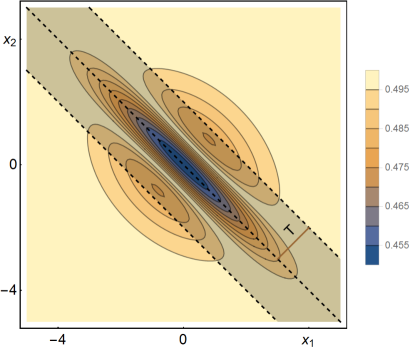
Figure 1: (Color Online) Contourplot of $P_{\hbox{\tiny Q}\,}(x_{1},x_{2})$ for a STS. The dark region between the two dashed parallel lines represents a choice of ${\mathcal{D}}_{c}$, the region of outputs associated to the inference of common noise. States and channel parameters are set as follows: $\epsilon=1,\gamma=0.7,\lambda_{1}=\lambda_{2}=\lambda=1,t=1$.

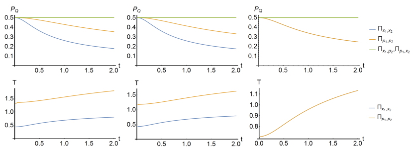
Figure 2: (Color Online) Upper panels: Error probability $P_{\hbox{\tiny Q}\,}$ for different POVMs for (left) STS ($\epsilon=1,\gamma=0.7$), (center) SV ($n=1,r=0.7$) and (right) standard SV ($n=1,r=0.7$). The POVM $\Pi(x_{1},x_{2})$(blue lower line) is always the most efficient. The POVMs $\Pi(x_{1},p_{2})$ and $\Pi(p_{1},x_{2})$ (upper red and green) yield the same error probability $P_{\hbox{\tiny Q}\,}=\frac{1}{2}$ independently on the input state and are useless for discrimination purposes. Lower panels: Optimal half-width $T$ as a function of time for POVMs $\Pi(x_{1},x_{2})$ and $\Pi(p_{1},p_{2})$. We set $\lambda_{1}=\lambda_{2}=\lambda=1$.

In section II, we have analyzed the dynamics in the presence of either local or common noise. The two dynamical maps are different and, in particular, correlations between the two oscillators appear exclusively in the common noise scenario, as it is apparent from the presence of off-diagonal terms in the common noise matrix. As a matter of fact, the correlation terms in the noise matrix corresponds the variances $var(X_{1},X_{2})$ and $var(P_{1},P_{2})$, where $X_{j}=\frac{1}{\sqrt{2}}(a_{j}+a^{\dagger}_{j}),P_{j}=\frac{1}{i\sqrt{2}}(a_{j}-a^{\dagger}_{j})$ are the quadrature operators of the two oscillatos. This argument suggests that joint homodyne detection of the quadratures of the two modes may be a suitable building block to discriminate the two possible environmental scenarios. In the following, we are about to consider the measurement of all possible combinations of quadratures, $(X_{1},X_{2})$, $(P_{1},P_{2})$, $(X_{1},P_{2})$ and $(P_{1},X_{2})$ and denote the corresponding POVMs as $\Pi(q_{1},q_{2})=|q_{1},q_{2}\rangle\rangle\langle\langle q_{1},q_{2}|\equiv|q_{1}\rangle\langle q_{1}|\otimes|q_{2}\rangle\langle q_{2}|$ with $q_{j}\in\{x_{j},p_{j}\}$, $j=1,2$ and $|q_{j}\rangle$ being quadrature eigenstates. In order to implement a discrimination strategy, we should define an inference rule connecting each possible outcome of the measurement to one of the two hypothesis: $H_{{\hbox{\tiny L}\,}}$, the noise is due to local interaction or $H_{\hbox{\tiny C}\,}$, the noise is due to common interaction with the environment. If we denote by ${\mathcal{D}}_{c}\subset{\mathbb{R}}^{2}$ the region of outcomes leading to $H_{\hbox{\tiny C}\,}$, i.e. to infer a common noise, then the two-value POVM describing the overall discrimination strategy is given by $E_{\hbox{\tiny C}\,}+E_{\hbox{\tiny L}\,}={\mathbb{I}}$, where

$$E_{\hbox{\tiny C}\,}=\int\!\!\!\int_{\mathcal{D}_{c}}\!\!dq_{1}dq_{2}\,\Pi(q_{1},q_{2})\qquad E_{{\hbox{\tiny L}\,}}={\mathbb{I}}-E_{\hbox{\tiny C}\,}\,.$$ (43)

The success probabilities, i.e. those of inferring the correct kind of noise are given by $P_{j}=\hbox{Tr}[\rho_{j}\,E_{j}]$, $j=L,C$ respectively, whereas the error probability, i.e. the probability of chosing the wrong hypothesis is given by

$$p_{\hbox{\tiny Q}\,} =\frac{1}{2}\big{(}\hbox{Tr}[\rho_{\hbox{\tiny L}\,}\,E_{\hbox{\tiny C}\,}]+\hbox{Tr}[\rho_{\hbox{\tiny C}\,}\,E_{\hbox{\tiny L}\,}]\big{)}$$

$$=\frac{1}{2}\left(1-\int\!\!\!\int_{\mathcal{D}_{c}}\!\!dq_{1}dq_{2}\,\hbox{Tr}\left[\Pi(q_{1},q_{2})\,(\rho_{\hbox{\tiny C}\,}-\rho_{\hbox{\tiny L}\,})\right]\right)$$ (44)

distribution of $(q_{1},q_{2})$.

The smaller is $P_{\hbox{\tiny Q}\,}$, the more effective is the discrimination strategy. In order to suitably choose $\mathcal{D}_{c}$ we have analyzed the behavior of the quantity

$$p_{\hbox{\tiny Q}\,}(q_{1},q_{2})=\hbox{Tr}\left[\Pi(q_{1},q_{2})\,(\rho_{\hbox{\tiny C}\,}-\rho_{\hbox{\tiny L}\,})\right],$$

in the $(q_{1},q_{2})$ plane. In Fig. 1 we show a contourplot of $p_{\hbox{\tiny Q}\,}(x_{1},x_{2})$ for a given input STS. This probability is squeezed along the $x_{1}x_{2}$ direction, since a common environment induces the build-up of correlations between the quadratures. For this reason, we choose ${\mathcal{D}}_{c}$ as the region between two straight lines at $45^{\circ}$ and denote by $T$ its half-width. The same argument holds also for SV and standard SV.

In the top panels of Fig. 2 we show a comparison between the error probability of the four POVMs described above on some particular STSs (left), standard form SVs (center) and SVs (right). As it is apparent from the plot, the POVMs $\Pi(x_{1},p_{2})$ and $\Pi(p_{1},x_{2})$ are useless. In fact, the common environment does not correlate these couples of quadratures. On the other hand, the POVM $\Pi(x_{1},x_{2})$, represented by the blue lines, always outperforms $\Pi(p_{1},p_{2})$. In the lower panels, we show the optimal values of the half-width $T$ of the region $\mathcal{D}_{c}$ as a function of the interaction time for the very same states.

V Random input Gaussian states

In this section, we address the optimization of the discrimination protocol using Gaussian states as input and the optimal homodyne-based POVM $\Pi(x_{1},x_{2})$. The main purpose is to figure out which Gaussian state leads to the optimal discrimination protocol and understand which lab-friendly states, among the classes of STSs, SVs and SSVs, are the most performant ones. We also analyze whether the efficiency of the discrimination protocol is affected by some relevant properties of the input states. To this aim we evaluate the error probability $P_{Q}$ as a function of energy and entanglement, at fixed purity. We recall that the energy $E$ and purity $\mu$ of a zero-mean valued two-mode Gaussian state with covariance matrix $\boldsymbol{\sigma}$ are given by

$$E(\boldsymbol{\sigma}) =\mbox{Tr}\Big{(}\frac{\boldsymbol{\sigma}}{2}\Big{)}-1$$

$$\mu(\boldsymbol{\sigma}) =\frac{1}{4\sqrt{\mbox{det}\boldsymbol{\sigma}}},$$ (45)

while the entanglement may be easily determined on the base of the PPT-criterion and quantified by the logarithmic negativity, which is given by

$$\mathcal{N}=\mbox{max}\{0,-\log(2\tilde{d}_{1})\}$$

where $\tilde{d}_{1}$ indicates the smallest symplectic eigenvalue of the partially transposed covariance matrix. In this paper, we prefer to directly use $\tilde{d}_{1}$ as a quantifier for entanglement: when $\tilde{d}_{1}<1/2$, the state is entangled, otherwise it is not.

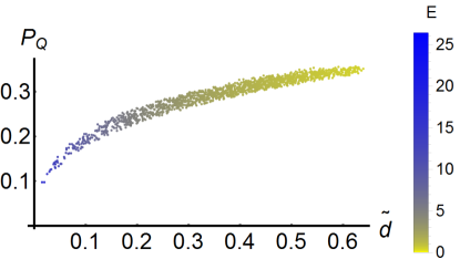
Figure 3: (Color Online) Error probability $P_{Q}$ for random Gaussian input states as a function of the smallest symplectic eigenvalue $\tilde{d}_{1}$ with POVM $\Pi(x_{1},x_{2})$. The color scale classifies the initial energy of the state. The error probability scales with the entanglement and the energy of the input state. We set $\lambda_{1}=\lambda_{2}=\lambda=1,t=1$.

In Fig. 3, we report the error probability of randomly generated Gaussian states in standard form with purity $\mu=0.6$ at fixed time $t=1$ as a function of the symplectic eigenvalue $\tilde{d}_{1}$ of the input state, while the color scale classifies its initial energy. As is apparent from the figures, for non-unitary purity, generating an always more entangled input state does not necessarily imply an improvement in the efficiency of the discrimination protocol. The same happens with energy: the error probability does not scale monotonicly with the energy stored in the input state. Nevertheless, if we increase the energy and the entanglement of the input state at the same time, the error probability lowers monotonicly.

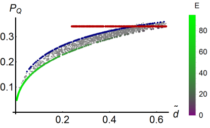
Figure 4: (Color Online) Error probability $P_{Q}$ as a function of the smallest symplectic eigenvalue $\tilde{d}_{1}$ with POVM $\Pi(x_{1},x_{2})$ for standard form random Gaussian states (gray dots), STSs (blue upper curve), SVs (red straight line) and SSVs (lower line). The color scale classifies the energies of the SSV states. The error probability of SV states does not depend on the entanglement of the input state. The most performant states are the SSVs. We set $\lambda=1$.

In Fig. 4 we show how efficient STSs, SVs and SSVs are with respect to all possible Gaussian states with the same purity ($\mu=0.6$). As a result, the most performant states are the SSVs: these states form a lower bound for every random-generated state, so representing the topmost suitable class state for discrimination protocols. One might make a conjecture that for SSVs entanglement might be the only resource to discrimination: unfortunately, this is true as long as purity is fixed, as the energy of SSVs monotonicly increases with entanglement, but false in general. Concerning SVs and STSs, it is worth noting that STSs are easily outperformed by any other standard form Gaussian state and that the error probability achieved with input SV states is not affected by a change in the initial entanglement (we want to remember that SVs’ covariance matrix is not in standard form, this explains why the red curve steps over the region of the standard form Gaussian states).

Finally, in Fig. 5 we compare the error probability achieved by some lab-friendly states with the bounds we introduced in sec III. In particular, we choose some highly performant identically entangled STS and SSV. The upper panel shows a comparison between the error probability for a STS with the fidelity and the Quantum Chernoff Bound. The double homodyne measurement yields an error probability (green line) that beats the Quantum Chernoff Bound (red line), The lower panel shows a similar comparison for a SV state. In this case, even though the SV state yields a lower error probability than a STS does, the QCB can only be saturated in the early dynamics.

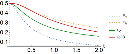
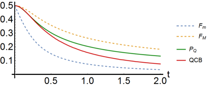
Figure 5: (Color Online) Comparison between error probability and fidelity and QCB bounds for STS state (upper panel) and SSV state (lower panel). In both panels, the dashed lines represent the upper bound $\mathcal{F}_{M}$ (orange line) and lower bound $\mathcal{F}_{m}$ (blue line), the green line represents the error probability $P_{Q}$, the red line represents the QCB. Upper panel: we set $\epsilon=1.956,\gamma=0.6593,\lambda=1.0$. Lower panel: we set $n=0.3333,r=1.470,\lambda=1$.

VI Conclusions

In conclusion, we have addressed the design of effective strategies to discriminate between the presence of local or common noise effect for a system made of two harmonic quantum oscillators interacting with classical stochastic fields. The commoin noise scenario corresponds to the interaction of the two-mode quantum system with a common classical field, whereas the local one is described by coupling the oscillators to independent classical fields.

We have shown that a discrimination protocol based on joint homodyne detection of the position operators yields an error probability that may outperform the Quantum Chernoff Bound, leading to a probability of error close to the Helstrom bound. In particular, we have shown that the QCB can be overtaken by means Gaussian states feasible with current technology.

Finally, we have shown that the error probability achieved with joint homodyne measurement strictly depends on the properties of the input state, as it lowers monotonicly with the energy and the entanglement of the input state.

- (1) U. Weiss Quantum Dissipative Systems (World Scientific, Singapore, 1999).
- (2) H. P. Breuer, F. Petruccione The Theory of Open Quantum Systems (Oxford University Press, Oxford, 2003).
- (3) S. Haroche and J.-M. Raimond Exploring the Quantum (Oxford University Press, Oxford, 2006).
- (4) W. H. Zurek,”Decoherence and the transition from quantum to classical” Phys. Today 44, 36 (1991).
- (5) J. P. Paz, S. Habib, and W. H. Zurek, ”Reduction of the wave packet: Preferred observable and decoherence time scale”, Phys. Rev. D 47, 488 (1993).
- (6) M. G. A. Paris, A. Serafini, F. Illuminati, S. De Siena, ”Purity of Gaussian states: measurement schemes and time–evolution in noisy channels”, Phys. Rev. A 68, 012314 (2003).
- (7) A. Serafini, S. De Siena, F. Illuminati, and M. G. A. Paris, ”Minimum decoherence cat-like states in Gaussian noisy channels”, J. Opt. B. 6, S591 (2004).
- (8) A. Serafini, F. Illuminati, M. G. A. Paris, S. De Siena, ”Entanglement and purity of two–mode Gaussian states in noisy channels”, Phys. Rev A 69, 022318 (2004).
- (9) T. Yu, J. H. Eberly, ”Entanglement Evolution in a Non-Markovian Environment” Opt. Comm. 283, 676 (2010).
- (10) D. Braun, ”Creation of Entanglement by Interaction with a Common Heat Bath”, Phys. Rev. Lett. 89 277901 (2002).
- (11) Y. Zhao, G.H. Chen, ”Two oscillators in a dissipative bath”, Physica A 317, 13 (2003).
- (12) F. Benatti, R. Floreanini, M. Piani, ”Environment in- duced entanglement in Markovian dissipative dynamics”, Phys. Rev. Lett. 91, 070402 (2003).
- (13) J. S. Prauzner-Bechcicki, ”Two-mode squeezed vacuum state coupled to the common thermal reservoir”, J. Phys. A: Math. Gen. 37, L173 (2004).
- (14) L. D. Contreras-Pulido, R. Aguado, ”Entanglement between charge qubits induced by a common dissipative environment”, Phys. Rev. B 77, 155420 (2008).
- (15) J. P. Paz, A. J. Roncaglia, ”Dynamics of the Entanglement between Two Oscillators in the Same Environment”, Phys. Rev. Lett. 100, 220401 (2008).
- (16) M. Brownnutt, M. Kumph, P. Rabl and R. Blatt, ”Ion-trap measurements of electric-field noise near surfaces”, Rev. Mod. Phys. 87, 1419 (2015).
- (17) S. Groeblacher, A. Trubarov, N. Prigge, G. D. Cole, M. As- pelmeyer, J. Eisert, ”Observation of non-Markovian micromechanical Brownian motion”, Nature Comm. 6, 7606 (2015).
- (18) G. M. Palma, K.-A. Suominen, A. K. Ekert ”Quantum Computers and Dissipation”, Proc. R. Soc. London A 452, 567 (1996).
- (19) A. Rivas, M. Muller, ”Quantifying spatial correlations of general quantum dynamics”, New J. Phys. 17, 062001 (2015).
- (20) P. Zanardi, M. Rasetti, ”Noiseless Quantum Codes” Phys. Rev. Lett. 79, 3306 (1997).
- (21) L.-M. Duan, G.-C. Guo, ”Preserving Coherence in Quantum Computation by Pairing Quantum Bits”, Phys. Rev. Lett. 79, 1953 (1997).
- (22) P. G. Kwiat, A. J. Berglund, J. B. Altepeter, A. G. White, ”Experimental verification of decoherence-free subspaces”, Science 290, 498 (2000).
- (23) R. H. Dicke, ”Coherence in Spontaneous Radiation Processes”, Phys. Rev.93, 99 (1954).
- (24) J. T. Barreiro et al. ”An open-system quantum simulator with trapped ions”, Nature 470, 486 (2011).
- (25) F. Verstraete, M. M. Wolf, J. I. Cirac, ”Quantum computation and quantum-state engineering driven by dissipation”, Nature Phys. 5, 633 (2009).
- (26) C.W. Gardiner, Handbook of Stochastic Methods, (Springer, Berlin, 1983).
- (27) J. Helm and W. T. Strunz ”Quantum decoherence of two qubits”, Phys. Rev. A 80, 042108 (2009).
- (28) J. Helm, W. T. Strunz, S. Rietzler, and L. E. Würflinger ”Characterization of decoherence from an environmental perspective”, Phys. Rev. A 83, 042103 (2011).
- (29) D. Crow and R. Joynt ”Classical simulation of quantum dephasing and depolarizing noise”, Phys. Rev. A 89, 042123 (2014).
- (30) W. M. Witzel, K. Young, and S. Das Sarma ”Converting a real quantum spin bath to an effective classical noise acting on a central spin”, Phys. Rev. B 90, 115431 (2014).
- (31) W. T. Strunz, L. Díosi, and N. Gisin ”Open System Dynamics with Non-Markovian Quantum Trajectories”, Phys. Rev. Lett. 82, 1801 (1999).
- (32) J. T. Stockburger and H. Grabert ”Exact c-Number Representation of Non-Markovian Quantum Dissipation”, Phys. Rev. Lett. 88, 170407 (2002).
- (33) Q.A. Turchette, C. J. Hyatt, B.E. King, C. A. Sackett, D. Kielpinski, W. M. Itano, C. Monroe and D. J. Wineland ”Decoherence and decay of motional quantum states of a trapped atom coupled to engineered reservoirs”, Phys. Rev. A 62, 053807 (2000).
- (34) O. Astafiev, Yu. A. Pashkin, Y. Nakamura, T. Yamamoto, and J. S. Tsai ”Quantum Noise in the Josephson Charge Qubit”, Phys. Rev. Lett. 93, 267007 (2004).
- (35) Y. M. Galperin, B. L. Altshuler, J. Bergli, and D. V. Shantsev ”Non-Gaussian Low-Frequency Noise as a Source of Qubit Decoherence”, Phys. Rev. Lett. 96, 097009 (2006).
- (36) B. Abel and F. Marquardt ”Decoherence by quantum telegraph noise: A numerical evaluation”, Phys. Rev. B 78, 201302(R) (2008).
- (37) T. Grotz, L. Heaney and W.T. Strunz ”Quantum dynamics in fluctuating traps: Master equation, decoherence, and heating”, Phys. Rev. A, 74, 022102 (2006).
- (38) J. Trapani, M.G.A. Paris, ”Non-divisibility vs backflow of information in understanding revivals of quantum correlations for continuous-variable systems interacting with fluctuating environments”, Phys. Rev. A 93, 042119 (2016).
- (39) C. W. Helstrom, Quantum Detection and Estimation Theory (Academic, New York, 1976).
- (40) K. M. R. Audenaert, M. Nussbaum, A. Szkola, and F. Verstraete, Commun. Math. Phys. 279, 251 (2008).
- (41) S. Pirandola and S. Lloyd, Phys. Rev. A 78, 012331 (2008).
- (42) J. Calsamiglia, R. Munoz-Tapia, L. Masanes, A. Acin, and E. Bagan, Phys. Rev. A 77, 032311 (2008).
- (43) K. M. R. Audenaert, J. Calsamiglia, R. Munoz-Tapia, E. Bagan, Ll. Masanes, A. Acin, F. Verstraete, Phys. Rev. Lett. 98, 160501 (2007).
- (44) C. Wittmann, U. L. Andersen, M. Takeoka, D. Sych, G. Leuchs, ”Discrimination of binary coherent states using a homodyne detector and a photon number resolving detector”, Phys. Rev. A 81, 062338 (2010).
- (45) S. Olivares, S. Cialdi, F. Castelli, M.G.A. Paris, ”Homodyne detection as a near-optimum receiver for phase-shift-keyed binary communication in the presence of phase diffusion”, Phys. Rev. A 87, 050303(R), (2013).
- (46) S. Pirandola, ”Quantum Reading of a Classical Digital Memory”, Phys. Rev. Lett. 106 , 090504 (2011).