Wormholes and black universes without phantom fields
in Einstein-Cartan theory

K. A. Bronnikov^a,b,c,1 and A. M. Galiakhmetov^d,2

^a

VNIIMS, Ozyornaya ul. 46, Moscow 119361, Russia

^b

Peoples’ Friendship University of Russia, ul. Miklukho-Maklaya 6, Moscow 117198, Russia

^c

National Research Nuclear University “MEPhI” (Moscow Engineering Physics Institute), Moscow, Russia

^d

Donetsk National Technical University, ul. Kirova 51, 84646, Gorlovka, Ukraine

We obtain a family of regular static, spherically symmetric solutions in Einstein–Cartan theory with an electromagnetic field and a nonminimally coupled scalar field with the correct sign of kinetic energy density. At different values of its parameters, the solution, being asymptotically flat at large values of the radial coordinate, describes (i) twice asymptotically flat symmetric wormholes, (ii) asymmetric wormholes with an AdS asymptotic at the “far end”, (iii) regular black holes with an extremal horizon or two simple horizons, and (iv) black universes with a de Sitter asymptotic at the “far end”. As in other black universe models, it is a black hole as seen by a distant observer, but beyond its horizon there is a nonsingular expanding universe. In all these cases, both the metric and the torsion are regular in the whole space.

Keywords: Einstein–Cartan theory, scalar field, nonminimal coupling, wormholes, regular black holes, black universes

PACS number: 04.20.-q, 04.20.Jb, 04.40.-b, 98.80.Jk

1 Introduction

The origin of the presently observed accelerated expansion of the Universe has become one of the most important problems in modern cosmology and even in theoretical physics as a whole. Among different theoretical models trying to explain it (see, e.g., the recent reviews [1–4] and references therein), two main trends can be distinguished: (1) introduction of a new hypothetic form of matter with large negative pressure, called dark energy (DE), in the framework of general relativity (GR) (the cosmological constant, various kinds of quintessence, phantom matter etc.), and (2) different suggestions in alternative theories of gravity, such as $f(R)$ theories, multidimensional theories and theories involving non-Riemannian geometries, such as the Riemann-Cartan geometry with torsion. The simplest theory of this kind is the Einstein-Cartan theory (ECT) [5–8], also leading to models of accelerated expansion [9–11].

The ECT can be considered as a degenerate version [12–14] of the Poincaré gauge theory of gravity (PGTG), in which the gravitational Lagrangian contains invariants quadratic in the curvature and torsion tensors. Unlike that, in the ECT the torsion is not dynamic since its gravitational action reduces to the curvature scalar of Riemann–Cartan space–time, directly generalizing the action of GR. It is nevertheless a viable theory of gravity: its observational predictions agree with the classical tests of GR, but it substantially differs from GR at very high densities of matter [8, 15, 16].

Theories with torsion also attract attention since torsion naturally arises in many approaches such as supergravity [17–19] and superstring [20–22] theories. One of the simplest extensions of the ECT is $f(R)$ gravity with torsion [23, 24], and, as shown in [24], torsion can play the role of DE and cause an accelerated expansion of the Universe.

Moreover, the existence of bouncing cosmologies in the ECT [11] shows that torsion can replace “exotic” sources, violating the weak and null energy conditions (WEC and NEC). As is well known, such a violation is in GR a necessary condition for the existence of traversable wormholes [25]. Wormholes are a subject of particular interest as possible time machines or shortcuts between different universes or distant parts of the same universe, for reviews see [26, 27, 28] and references therein.

Quite a number of wormhole solutions are known, see, e.g, [29–32] for solutions with minimally coupled scalar fields, [29, 33] for solutions with conformal coupling and [34, 35, 36] for other couplings. In agreement with the general results [25], minimally coupled scalar fields supporting wormholes have to be phantom (i.e., have a wrong sign of kinetic energy). In the case of a nonminimal coupling, there are special wormhole solutions with normal fields, but in all such cases there are always regions where the effective gravitational constant becomes negative, that is, the gravitational field itself becomes a phantom [37, 38]. Moreover, all such configurations, whose existence is connected with the phenomenon of conformal continuation [39, 37], turn out to be unstable under radial perturbations [40, 36, 41].

Some extensions of GR predict the existence of wormholes without exotic matter, in particular, brane world models [42, 43], Einstein-Gauss-Bonnet gravity [44] and other high-order theories [45], the Horndeski theory [46] and others.

From the properties of the ECT it is also natural to expect that in this theory wormholes can exist without exotic matter or at least without manifestly phantom fields with a wrong sign of kinetic energy. And indeed, a family of exact static, spherically symmetric wormhole solutions in the ECT was recently found [47] with a pair of canonical scalar fields as sources of gravity. One of these fields was nonminimally coupled to Riemann-Cartan curvature and provided the effect of torsion on the space-time metric. A shortcoming of these solutions was an infinite value of the torsion scalar at the wormhole throat.

Other kinds of configurations in GR whose existence is connected with NEC and WEC violation are regular black holes which, instead of a singularity at $r=0$, contain, at the “far end”, flat or (anti-) de Sitter asymptotic regions [31, 48, 32]. Among them of particular interest are the so-called black universes. By definition, a black universe is a nonsingular black hole in which, beyond the event horizon, there is an expanding universe. This class of models provides avoidance of singularities in both black holes and cosmology and combines the properties of a wormhole (absence of a center, a regular minimum of the area function in the case of spherical symmetry) and a black hole (a horizon separating static and cosmological regions of space-time). Moreover, the Kantowski-Sachs cosmology in the T region can be asymptotically isotropic and approach a de Sitter mode of expansion, which makes such models potentially viable for a description of an inflationary Universe or the present accelerated expansion. A number of such solutions of GR have been obtained with different kinds of phantom scalar fields as sources, with and without electromagnetic fields [31, 32, 49, 50].

In the present study, we again seek static, spherically symmetric solutions in the ECT but now with a single nonminimally coupled scalar field (being a source of torsion) and an electromagnetic field. Our purposes are (1) to obtain both wormhole and regular black hole solutions with a normal scalar field, (2) to include electric or magnetic fields into consideration, and (3) to avoid a singular behavior of torsion in the whole space-time.

The paper is organized as follows. In Section 2 we present the ECT equations both in the general case and for static, spherically symmetric configurations involving an electromagnetic field and a scalar field nonminimally coupled to space-time curvature. Section 3 is devoted to finding and analyzing the properties of a family of exact solutions, and Section 4 is a discussion.

2 Field equations

We start with the action

$${}S=\int\sqrt{-g}d^{4}x\Bigl{[}-\frac{R}{2\kappa}+\frac{\eta}{2}\Bigl{(}\phi_{,k}\phi^{,k}+\xi R\phi^{2}\Bigr{)}$$

$${}\hskip 72.26999pt-V(\phi)-\frac{1}{4}F_{ik}F^{ik}\Bigr{]},$$ (1)

where $R=R[\Gamma]$ is the curvature scalar obtained from the full connection $\Gamma^{k}_{ij}=\{^{k}_{ij}\}+S_{ij\cdot}^{\ \ {k}}+S^{k}_{\cdot{ij}}+S^{k}_{\cdot{ji}}$; here $\{^{k}_{ij}\}$ are Christoffel symbols of the second kind for the metric $g_{ik}$; $S_{ij\cdot}^{\ \ {k}}=\Gamma^{k}_{[ij]}$ is the torsion tensor; $\kappa=8\pi G$, $G$ being the Newtonian gravitational constant; $\phi$ is a scalar field with the potential $V(\phi)$; $F_{ik}$ is the Maxwell tensor. The constant $\eta=\pm 1$ corresponds to either a usual, canonical scalar field ($\eta=+1$) or to a phantom one ($\eta=-1$).

The metric $g_{ik}$ has the signature ($+\ -\ -\ -$), the Riemann and Ricci tensors are defined as

$$R^{\ \ \ m}_{ijk\cdot}=\Gamma^{m}_{jk,i}-\Gamma^{m}_{ik,j}+\Gamma^{m}_{ip}\Gamma^{p}_{jk}-\Gamma^{m}_{jp}\Gamma^{p}_{ik}$$

and $R_{jk}=R^{\ \ \ i}_{ijk\cdot}$. We should note that in ECT a scalar field nonminimally coupled to gravity gives rise to torsion even though it has zero spin. It follows from (2) that torsion can interact with a scalar field only through its trace: $S_{i}=S_{ik\cdot}^{\ \ k}$ (see [51]). Hence, the curvature scalar $R(\Gamma)=g^{jk}R_{jk}$ can be presented in the form [51]

$$R[\Gamma]=R[\{\}]+4\nabla_{k}S^{k}-(8/3)S_{k}S^{k}\ ,$$ (2)

where $R[\{\}]$ is the Riemannian part of the curvature built from the Christoffel symbols, and $\nabla_{k}$ is the covariant derivative of Riemannian space.

Since torsion is induced by a nonminimally coupled scalar field only, the tensor $F_{ik}$ is gauge-invariant: $F_{ik}=\partial_{i}A_{k}-\partial_{k}A_{i}$, where $A_{i}$is the potential four-vector of the electromagnetic field.

Varying the action with the Lagrangian (2) in $g_{ij}$, $S_{k}$, $\phi$, $\psi$ and $A_{k}$, we obtain the following set of equations:

$${}G_{ij}[\{\}]=\kappa(T_{ij}[\phi]+T_{ij}[e])+\Lambda_{ij},$$ (3)

$${}S^{k}=\frac{3}{2}\xi\Psi\phi\phi^{,k},$$ (4)

$${}\Box\phi-\xi\phi R[\Gamma]+\eta dV/d\phi=0,$$ (5)

$${}\frac{1}{\sqrt{-g}}\partial_{i}(\sqrt{-g}F^{ik})=0,$$ (6)

where

$${}T_{ij}[\phi]=\eta\biggl{\{}\phi_{,i}\phi_{,j}-\frac{1}{2}\Big{[}\phi_{,m}\phi^{,m}+\xi R[\{\}]\phi^{2}$$

$${}\ \ \ -2\eta V(\phi)\Big{]}\,g_{ij}+\xi\Big{[}-4S_{(i}\nabla_{j)}+2g_{ij}S^{n}\nabla_{n}$$

$${}\ \ \ -\nabla_{i}\nabla_{j}+g_{ij}\Box+R_{ij}[\{\}]-\Lambda_{ij}\Big{]}\phi^{2}\biggr{\}},$$ (7)

$${}T_{ij}[e]=-F^{k}_{i}F_{jk}+\frac{1}{4}F_{lk}F^{lk}g_{ij},$$ (8)

$${}\Lambda_{ij}=\frac{8}{3}S_{i}S_{j}-\frac{4}{3}S_{k}S^{k}g_{ij}.$$ (9)

Here $\Box$ is the d’Alembertian operator of Riemannian space, and we denote $\Psi=\kappa(\eta-\kappa\xi\phi^{2})^{-1}$.

It is easy to verify that the effective scalar-torsion stress-energy tensor (SET) $T^{\rm(eff)}_{ij}[\phi]$

$$T^{\rm(eff)}_{ij}[\phi]=T_{ij}[\phi]+\kappa^{-1}\Lambda_{ij}$$ (10)

as well as the electromagnetic SET $T_{ij}[e]$ are separately covariantly conserved since no explicit coupling is assumed between the scalar and electromagnetic fields:

$$\nabla^{j}T^{\rm(eff)}_{ij}[\phi]=\nabla^{j}T_{ij}[e]=0.$$ (11)

The general static, spherically symmetric metric can be written in the form

$$ds^{2}=A(u)dt^{2}-\frac{du^{2}}{A(u)}-r^{2}(u)d\Omega^{2}$$ (12)

in terms of the so-called quasiglobal radial coordinate [28], where $g_{00}=A(u)$ may be called the redshift function while $r(u)$ is the area function, or spherical radius; $d\Omega^{2}=d\theta^{2}+\sin^{2}\theta d\varphi^{2}$ is the linear element on a unit sphere. (As usual, the metric is only formally static: it is really static if $A>0$, but it describes a Kantowski–Sachs (KS) type cosmology if $A<0$, and $u$ is then a temporal coordinate.) We also consider $\phi=\phi(u)$.

The nonvanishing components of the effective scalar-torsion SET are given by

$${}T^{1\ \rm(eff)}_{1}[\phi]=\eta\xi\phi^{2}G^{1}_{1}[\{\}]+Y+\eta\Big{[}2\xi\phi\phi^{\prime\prime}A$$

$${}\quad\ +\xi\phi\phi^{\prime}A^{\prime}+(-1+2\xi+6\xi^{2}\phi^{2}\Psi)\phi^{\prime 2}A\Big{]},$$ (13)

$${}T^{2\ \rm(eff)}_{2}[\phi]=T^{3\rm(eff)}_{3}[\phi]$$

$${}\quad\ =\eta\xi\phi^{2}G^{2}_{2}[\{\}]+Y+2\eta\xi\frac{r^{\prime}}{r}\phi\phi^{\prime}A,$$ (14)

$${}T^{0\rm(eff)}_{0}[\phi]=\eta\xi\phi^{2}G^{0}_{0}[\{\}]+Y+\eta\xi\phi\phi^{\prime}A^{\prime},$$ (15)

where the prime means $d/du$ and

$${}Y=V(\phi)+\eta A\biggl{[}-2\xi\phi\phi^{\prime\prime}-2\xi\Bigl{(}\frac{A^{\prime}}{A}+\frac{2r^{\prime}}{r}\Bigr{)}\phi\phi^{\prime}$$

$${}\hskip 72.26999pt+\Bigl{(}\frac{1}{2}-2\xi-3\xi^{2}\phi^{2}\Psi\Bigr{)}\phi^{\prime 2}\biggr{]},$$ (16)

and $G^{i}_{k}[\{\}]$ is the Einstein tensor of Riemannian space.

The electromagnetic field compatible with the metric (12) can have the nonzero components

$$F_{01}={-}F_{10}\ \mbox{(electric)\ and}\ F_{23}={-}F_{32}\ \mbox{(magnetic)},$$

such that

$$F_{01}F^{01}=-\frac{q^{2}_{e}}{r^{4}(u)},\quad F_{23}F^{23}=\frac{q^{2}_{m}}{r^{4}(u)},$$ (17)

where the constants $q_{e}$ and $q_{m}$ are the electric and magnetic charges, respectively. The corresponding SET is

$$T^{k}_{i}[e]=\frac{q^{2}}{r^{4}(u)}\mathop{\rm diag}\nolimits(1,1,-1,-1)\ ,$$ (18)

where $q^{2}=q^{2}_{e}+q^{2}_{m}$. Thus the electromagnetic field equations have already been solved.

The scalar field equation and three independent combinations of the Einstein–Cartan equations read

$${}(1-6\xi^{2}\phi^{2}\Psi)\frac{(Ar^{2}\phi^{\prime})^{\prime}}{r^{2}}-\frac{6\eta}{\kappa}\xi^{2}\phi\phi^{\prime 2}\Psi^{2}A$$

$${}\ \ \ -\eta\frac{dV}{d\phi}+\xi\phi\biggl{[}A^{\prime\prime}+\frac{4Ar^{\prime\prime}}{r}+\frac{4A^{\prime}r^{\prime}}{r}$$

$${}\hskip 72.26999pt+\frac{2Ar^{\prime 2}}{r^{2}}-\frac{2}{r^{2}}\biggr{]}=0,$$ (19)

$${}(A^{\prime}r^{2})^{\prime}=-2\eta r^{2}V\Psi+\frac{\eta q^{2}}{r^{2}}\Psi$$

$${}\ \ \ +2\xi r^{2}A\Psi\biggl{[}\phi\phi^{\prime\prime}+\phi^{\prime 2}+2\Bigl{(}\frac{A^{\prime}}{A}+\frac{r^{\prime}}{r}\Bigr{)}\phi\phi^{\prime}\biggr{]},$$ (20)

$${}2\frac{r^{\prime\prime}}{r}=\Psi\Big{[}2\xi\phi\phi^{\prime\prime}+(-1+2\xi+6\xi^{2}\phi^{2}\Psi)\phi^{\prime 2}\Big{]},$$ (21)

$${}A(r^{2})^{\prime\prime}-r^{2}A^{\prime\prime}=2-\frac{2\eta q^{2}}{r^{2}}\Psi$$

$${}\hskip 72.26999pt+2\xi r^{2}\phi\phi^{\prime}\Psi\Bigl{(}\frac{2Ar^{\prime}}{r}-A^{\prime}\Bigr{)}.$$ (22)

It should be noted that the scalar field equation (2) follows from (20)–(2).

We see that in the Einstein-Cartan equations (2)–(2) the terms induced by torsion contain the factor $\xi^{2}$, i.e., they exist due to nonminimal coupling of the $\phi$ field with space-time curvature.

3 Exact solution

Let us now try to solve Eqs. (20)–(2). Assuming $\eta=+1$ and $\xi>0$, the form of the expression for $\Psi$ and Eq. (21) prompts us to choose the following ansatz for $\phi$:

$$\phi(u)=\frac{1}{\sqrt{\kappa\xi}}\frac{u}{\sqrt{u^{2}+b^{2}}}=\frac{1}{\sqrt{\kappa\xi}}\frac{x}{\sqrt{x^{2}+1}}\ ,$$ (23)

where $x=u/b$, and $b>0$ is an arbitrary constant (the length scale). As a result, Eq. (21) takes the form

$$\frac{r^{\prime\prime}}{r}=\frac{2\xi-1}{2\xi(x^{2}+1)^{2}}\ ,$$ (24)

where the prime now stands for $d/dx$. Since in wormhole and black universe solutions the radius $r(x)$ should grow to infinity at both ends of the $x$ range, only solutions with $r^{\prime\prime}>0$ are admissible, therefore we choose $\xi>1/2$.

The general solution of Eq. (24) is [52]

$${}r(x)=b\sqrt{x^{2}+1}\ [\gamma\cos z+\beta\sin z]$$

$${}\hskip 28.45274pt\equiv\gamma b\sqrt{x^{2}+1}\cos z,$$

$${}z:=p\arctan x+\alpha,\quad\ p:=(2\xi)^{-1/2}<1,$$ (25)

where $\alpha$, $\beta$, $\gamma$ are integration constants. To obtain $r>0$ at all $x$, we suppose $\gamma>0$, and since there is an arbitrary factor $b$, without loss of generality we put $\gamma=1$. We also put

$$-\frac{\pi}{2}(1{-}p)\leq\alpha\leq\frac{\pi}{2}(1{-}p)\ \ \Rightarrow\ \ p\leq 1-\frac{2|\alpha|}{\pi}$$ (26)

(the second inequality is useful if $\alpha$ is known). Under these conditions (with strict inequality) $\cos z>0$ at all finite $x$, which leads to globally regular solutions.

From (3) it follows

$$\frac{r^{\prime}}{r}=\frac{x-p\tan z}{x^{2}+1},$$ (27)

so that $r^{\prime}=0$ where $x=p\tan z$. This value of $x$ is a minimum of $r(x)$ inside the range (26) of $\alpha$, while at its ends it is a limiting value at one of the infinities, see Fig. 1. This corresponds to what is sometimes called a “horn”: at one end $r$ tends to a constant. The function $r(x)$ is even if $\alpha=0$.

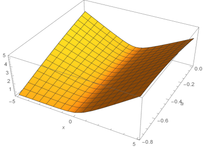
Figure 1: The function $r(x)$ for $p=1/2$ and $-\pi/4\leq\alpha\leq 0$.

The other metric function $A(x)$ is found from Eq. (2) which can be presented as

$${}B^{\prime\prime}+2B^{\prime}\ \frac{x-2p\tan z}{x^{2}+1}+\frac{2}{(x^{2}+1)^{2}\cos^{4}z}$$

$${}\hskip 28.45274pt-\frac{2Q}{(x^{2}+1)^{2}\cos^{6}z}=0,$$ (28)

where $Q=\kappa q^{2}/b^{2}$ and

$$B(x)=\frac{A(x)}{(x^{2}+1)\cos^{2}z}.$$ (29)

Its integration gives

$${}B(x)=B_{0}+\frac{1}{3p^{2}}\Bigl{[}\sec^{2}z-4\ln\cos z+\frac{3}{2}Q\sec^{4}z$$

$${}\hskip 28.45274pt-2(K+z)(2+\sec^{2}z)\tan z\Bigr{]},$$ (30)

where $B_{0}$ and $K$ are integration constants.

It is easy to see that in the general case (except for the limiting cases $\alpha=\pm(1-p)\pi/2$) $B(x)$ tends to finite limits as $x\to\pm\infty$, which, according to (29), leads to $A\sim x^{2}$ at both infinities, i.e., to de Sitter (dS) or AdS asymptotic behaviors. We will, however, restrict ourselves to discussing only systems which are asymptotically flat systems as $x\to+\infty$. Hence $B(x)\sim x^{-2}$, and in the expansion of $B(x)$ in inverse powers of $x$ the first two terms, $O(1)$ and $O(1/x)$, should vanish, which fixes the constants $B_{0}$ and $K$:

$${}6p^{2}B_{0}=8\ln\cos a-2\sec^{2}a$$

$${}\quad\ +Q\Big{[}{-}3\sec^{4}a+4\tan^{2}a(2+\sec^{2}a)\Big{]},$$ (31)

$${}K=-a+Q\tan a$$ (32)

where

$$a=\alpha+\pi p/2.$$ (33)

Under the conditions (3) and (32), we have the following expression for $A(x)$ at large positive $x$:

$${}A(x)=\Big{(}1+\frac{2p}{x}\tan a\Big{)}\biggl{[}\frac{Q-\cos^{2}a}{\cos^{4}a}$$

$${}\hskip 28.45274pt-\frac{2p(5Q-4\cos^{2}a)}{3x\cos^{5}a}\sin a\biggr{]}+O(x^{-2}).$$ (34)

It follows from (3) that the system can be asymptotically flat only if $Q>\cos^{2}a$, that is, only in the presence of an electromagnetic field.

Choosing properly the time scale at infinity and taking into account that $r\approx bx\cos a$ at large $x$, we obtain from (3) a Schwarzschild-like form of $g_{00}$:

$$\frac{A(x)}{A(\infty)}=1-\frac{2pb}{3r}\frac{2Q-\cos^{2}a}{Q-\cos^{2}a}\sin a,$$ (35)

and comparing it with the expression $1-2Gm/r$, we see that the Schwarzschild mass is

$$m=\frac{bp}{3l_{\rm pl}}m_{\rm pl}\frac{2Q-\cos^{2}a}{Q-\cos^{2}a}\sin a.$$ (36)

where $m_{\rm pl}=1/\sqrt{G}$ and $l_{\rm pl}=\sqrt{G}$ are the Planck mass and length, respectively. If we require $m\geq 0$, then from (36) it follows $a\geq 0$.

From Eq. (20) one derives the potential $V(x)$:

$${}V(x)=\frac{1}{3\kappa b^{2}(x^{2}+1)^{2}}\Bigl{[}4$$

$${}\hskip 28.45274pt+(3p^{2}B_{0}-4\ln\cos z)(4\cos^{2}z-3)$$

$${}\hskip 28.45274pt-4(K+z)(4\cos^{2}z-1)\tan z\Bigr{]}.$$ (37)

To express $V(x)$ in terms of $\phi$, by (23), we must put $x=\sqrt{\kappa\xi}\phi(1-\kappa\xi\phi^{2})^{-1/2}$.

Lastly, the expression for the squared trace of torsion $S^{2}=S_{k}S^{k}$ has the form

$$S^{2}=-\frac{9x^{2}A(x)}{4b^{2}(x^{2}+1)^{2}}\ .$$ (38)

Thus $S^{i}$ is a spacelike vector for $A>0$ and a timelike one for $A<0$, i.e., in a KS cosmology. For the solution (3), (3) the torsion is everywhere regular and finite; it is zero at $x=0$ which is a minimum of $r(x)$ if $\alpha=0$. At flat infinity the torsion invariant (38) decays by the law

$$S^{2}\Big{|}_{x\to+\infty}\sim x^{-2}\to 0\ .$$ (39)

At a dS/AdS infinity the invariant (38) tends to a nonzero constant.

Thus our solution (3), (3) under the conditions (3), (32) contains two integration constants $\alpha$ (or $a$) and $K$, which determine the mass $m$ and the dimensionless charge $Q=\kappa q^{2}/b^{2}$. There are also two free parameters $b>0$ (the length scale) and $p=(2\xi)^{-1/2}\in(0,1)$ characterizing the nonminimal coupling of the scalar field to curvature.

Of interest is the asymptotic value $B(-\infty)$: if it is negative, then the whole configuration is a black universe, otherwise it is either a wormhole (if $B(x)>0$ everywhere) or a regular black hole with a static region at large negative $x$. The expression for $B(-\infty)$ is very simple if we put $\alpha=0$, in which case the function $r(x)$ is even while $z(x)$ is odd. Indeed, under the conditions (3), (32) we have

$$B(-\infty)=\frac{4K}{3p^{2}}\tan a(2+\sec^{2}a)$$ (40)

By (36), $\mathop{\rm sign}\nolimits m=\mathop{\rm sign}\nolimits a$, hence if $m>0$, the sign of $B(-\infty)$ is determined by the sign of $K=Q\tan a-a$. For $Q$ we only have the inequality $Q>\cos^{2}a$, which allows the expression $Q\tan a-a$ to have any sign. We conclude that our solution can describe black universes with $m\geq 0$.

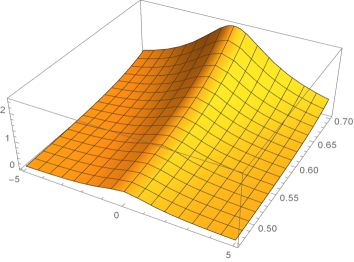
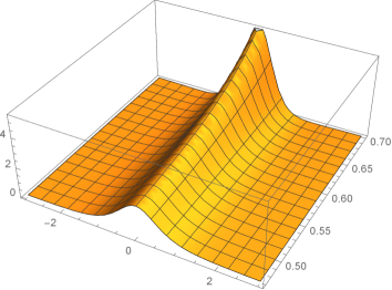
Figure 2: Plots of $B(x)$ (left) and $V(x)$ (right) for symmetric configurations with $p$ ranging from 0.47 to 0.7.

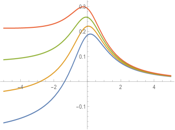
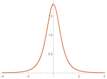
Figure 3: Plots of $B(x)$ (left) and $V(x)$ (right) for asymmetric configurations with even $r(x)$, and the parameters $p=0.4$, $Q=0.85,\ 0.86,\ 0.87,\ 0.88$ (bottom-up). The plots of $V(x)$ almost merge for these close values of the parameters though the corresponding geometries are qualitatively different.

In what follows we will briefly describe the properties of the solution for different values of its parameters under the conditions (3), (32).

3.1 Symmetric configurations

The solution is symmetric under the reflection $x\mapsto-x$ if and only if $\alpha=0$ and $K=0$. Then the only free parameters are the length scale $b$ and $p$, so that

$${}a=\pi p/2,\quad\ Q=a\cot a,$$

$${}Gm=\frac{2ab}{3\pi}\sin a\frac{4a-\sin(2a)}{2a-\sin(2a)}.$$ (41)

The solution exists for all $a\in(0,\pi/2)$, or $p\in(0,1)$, or $\xi>1/2$, and $Gm\in(b/\pi,2b/3)$.

Plots of $B(x)$ and $V(\phi)$ for different $p$ are shown in Fig. 2. Such symmetric configurations are asymptotically flat at both ends, $x\to\pm\infty$, and represent twice asymptotically flat (symbolically, M–M where “M” stands for “Minkowski”) traversable wormholes. Given the value of $b$, which is the throat radius, the Schwarzschild mass at both ends, found according to (41), is the smallest at $a\ll 1$, at which

$$Gm\approx Gm_{\min}=b/\pi.$$

It is easy to estimate that if we suppose that the wormhole is large enough for transportation purposes, say, $b=10$ m, then this minimum mass will be about $2.62\mbox{$\cdot 10^{30}$}$ g, about 440 Earth’s masses. The gravitational field in such a wormhole will be evidently too strong for a human being to survive.

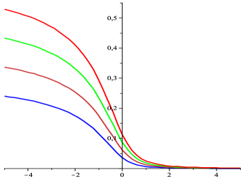
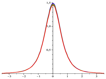
Figure 4: Plots of $B(x)$ (left) and $V(x)$ (right) for asymmetric configurations with $m=0$, $\alpha=-\pi/20$, $p=0.1$ and $Q=1.01,\ 1.02,\ 1.03,\ 1.04$ (bottom-up). The plots of $V(x)$ almost merge for these close values of the parameters.

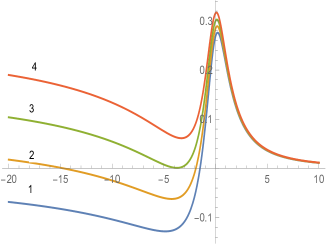
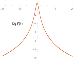
Figure 5: Plots of $B(x)$ (left) and $V(x)$ (middle and right) for asymmetric configurations with $\alpha=-\pi/48$, $p=0.5$ and $Q=0.813,\ 0.817,\ 0.821,\ 0.825$ (bottom-up). The plots of $V(x)$, as in other examples, almost merge. The right panel shows $\log V(x)$ in a wider range of $x$, which is possible due to $V>0$.

3.2 Asymmetric configurations with even $r(x)$

The condition $\alpha=0$ singles out the branch of our general solution with the even function
$r(x)=b\sqrt{x^{2}+1}\cos(p\arctan x)$, in which case we have, in addition to the length scale $b$, two free parameters $p$ and $Q$ and the limit (40) of $B(x)$ at negative infinity. Accordingly, we obtain two types of qualitatively different asymmetric configurations: M-AdS wormholes in which $B(-\infty)>0$ (they correspond to larger charges $Q$ at given $p$) and M-dS black universes with a single simple horizon and $B(-\infty)<0$ (at smaller $Q$ for given $p$). The corresponding functions $B(x)$ and $V(x)$ for some values of $p$ and $Q$ are plotted in Fig. 3. The two kinds of solutions are separated by the completely symmetric M-M wormhole solutions discussed in the previous subsection.

3.3 Asymmetric solutions with $\alpha\neq 0$

In this general case there are three parameters that affect the solution behavior, and accordingly the properties of geometries, qualitatively determined by the behavior of the function $B(x)$, are more diverse.

From $m\geq 0$ $(a\geq 0)$ it follows $\alpha\geq-\pi p/2$. Hence we should study two ranges of $\alpha$: (i) $-\pi p/2\leq\alpha<0$ and (ii) $0<\alpha<\pi(1{-}p)/2$.

1. At the lower bound, $\alpha=-\pi p/2$ $(p<1/2)$, the Schwarzschild mass is zero, $m=0$. The solution is asymptotically flat under the condition $Q>1$, and the only kind of configurations it describes are massless M–AdS wormholes. Examples of the behavior of $B(x)$ and $V(x)$ in this case are presented in Fig. 4.

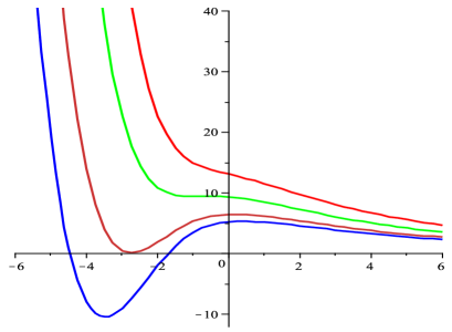
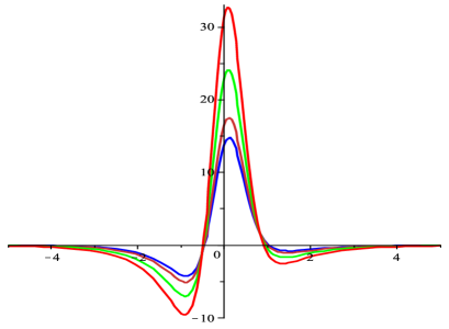
Figure 6: Plots of $B(x)$ (left) and $V(x)$ (right) for singular horn-like configurations with $\alpha=-\pi/20$, $p=0.9$ and $Q=0.37,\ 0.409,\ 0.5,\ 0.62$ (bottom-up both on the left panel and on the peak near $x=0$ on the right panel).

2. Consider a few examples with $\alpha<0$ and $m>0$. For some such examples we take $\alpha=-\pi/48$ and $p=0.5$, which implies $Q>0.56$. Trying different values of $Q$, we find its critical values that separate different modes of $B(x)$, as illustrated in Fig. 5. At smaller $Q$ (left panel, curve 1) we obtain a black universe (M-dS) with a single horizon. Larger values of $Q$ (curve 2) lead to regular M-AdS black holes with two simple horizons and a Reissner-Nordström-like global causal structure (with an AdS asymptotic at the far end, $x\to-\infty$, instead of a central singularity). Further slightly increasing the $Q$ value, we obtain a regular M-AdS black hole with a double horizon (curve 3). And lastly, at larger $Q$ we obtain M-AdS wormholes (curve 4).

An analysis shows that no other types of the behavior of $B(x)$ emerge at any admissible values of $\alpha$, both positive and negative, leading to finite $B(-\infty)$.

3. In the limiting case $\alpha=(p-1)\pi/2$, Eq. (3) shows that the solution describes a horn-like configuration with $r\to bp={\rm const}$ as $x\to-\infty$. In this case, due to the summand proportional to $\sec^{4}z$ in the expression for $B(x)$, at large negative $x$ we have $B(x)\sim x^{4}\to\infty$. Fig. 6 illustrates the properties of such configurations with $\alpha=-\pi/20$ and $p=9/10$. The metric function $A(x)$ also blows up as $x^{4}$ at the end of the “horn”, hence actually the distance to this end from any point is finite, $l=\int dx/\sqrt{A(x)}\sim\int dx/x^{2}<\infty$, and an inspection shows that there is a curvature singularity. The latter is repulsive, and, like the Reissner-Nordström singularity, can be naked (see the upper two curves in Fig. 6, left) or hidden beyond one extremal or two simple horizons (the lower two curves).

4 Concluding remarks

We have found a family of exact static, spherically symmetric solutions in the Einstein-Cartan theory (ECT) of gravity, with sources in the form of a nonminimally coupled non-phantom scalar field and an electromagnetic field. From this whole family we have selected asymptotically flat solutions with a nonnegative Schwarzschild mass. The remaining subfamily depends on four constants: the nonminimal coupling coefficient $\xi>1/2$, an arbitrary length scale $b>0$ and two significant integration constants: the dimensionless electromagnetic charge $Q$ and the “asymmetry factor” $\alpha$. With different values of these parameters, the solution describes (i) twice asymptotically flat (or M-M) symmetric wormholes, (ii) asymmetric M-AdS wormholes with zero or nonzero masses, (iii) regular M-AdS black holes with an extremal horizon or two simple horizons, and (iv) M-AdS black universes. It is important that, in all these solutions with a nonsingular metric, the torsion scalar also remains finite in the whole space, unlike the recently obtained wormhole solutions in the ECT with two scalars [47].

In addition, there are a number of singular solutions that remained beyond the scope of this study, for example, those with $\alpha$ outside the range (26). It seemed that if $\alpha$ takes a marginal value such that the spherical radius tends to a finite constant $r=r_{0}$ at the “far end”, $x\to-\infty$. It turns out, however, that such solutions possess a repulsive singularity at $r=r_{0}$, and, depending on $Q$, this singularity can be naked or hidden beyond horizons from the viewpoint of a distant observer.

It is clear that in our solutions the existence of a minimum of $r(x)$ (a throat) is provided by WEC and NEC violation by the effective SET (10) of the scalar–torsion field. A question of interest is whether or not the purely scalar SET respects the energy conditions, so that their violation might be completely ascribed to the contribution of torsion. We notice, however, that this question cannot be asked correctly because only the effective SET $T^{i\rm(eff)}_{k}[\phi]$ satisfies the conservation law (11), and the purely scalar contribution cannot be unambiguously separated from that of torsion.

Nevertheless, let us try to calculate the quantity $\rho+p_{r}\equiv T^{t}_{t}-T^{x}_{x}$ (whose negative value indicates NEC violation) for the purely scalar contribution in the SET (2), excluding there the terms containing $S$ and its derivatives, which would be a correct expression for the scalar field SET in the absence of torsion. We obtain

$$\rho[\phi]+p_{r}[\phi]=\frac{A(x)\bigl{[}1-2\xi+(1+4\xi)x^{2}\bigr{]}}{\kappa\xi b^{2}(x^{2}+1)^{2}}.$$ (42)

This expression is negative at small $x$ (near the throat) since $\xi>1/2$, but becomes positive far from it. This resembles the concept of a “trapped ghost” [49, 53], but, in contrast to these papers, here the kinetic term of the scalar field does not change its sign.

It is of interest that the effective density $\rho^{\rm(eff)}[\phi]=T^{t\rm(eff)}_{t}$ can be positive near the throat in our solution, so that NEC violation is caused by a larger negative value of the effective radial pressure $p_{r}^{\rm(eff)}[\phi]=-T^{x\rm(eff)}_{x}$ Thus, for symmetric configurations $(\alpha=0,\ K=0)$ we obtain at $x=0$

$$\rho^{\rm(eff)}[\phi]=\frac{1}{\kappa b^{2}}\Bigr{[}2+2(p^{2}-1)B_{0}+Q\Bigr{]}.$$ (43)

For $p=0.5$   $(a=Q=\pi/4)$ we have

$$\rho^{\rm(eff)}[\phi]=\frac{1}{\kappa b^{2}}\Bigr{[}6+4\ln 2-\frac{3\pi}{4}\Bigr{]}>0.$$ (44)

We conclude that the ECT, like some other extensions of GR, provides the existence of regular configurations without a center (wormholes, black universes, and regular black holes with two asymptotic regions) with normal (non-phantom) fields. It means that torsion here replaces (or plays the part of) exotic matter while forming such regular objects. A feature of interest in the present solution is the necessity of the electromagnetic field for obtaining asymptotic flatness, but it is evidently a property of the present family of solutions rather than a general property of the theory.

A challenging problem is that of stability of these and other solutions of the ECT, and we hope to deal with it in our further studies.

Acknowledgments

The work of KB was partly performed within the framework of the Center FRPP supported by MEPhI Academic Excellence Project (contract No. 02.a03.
21.0005, 27.08.2013). This paper was also financially supported by the Ministry of Education and Science of the Russian Federation on the program to improve the competitiveness of the RUDN University among the world leading research and education centers in 2016–2020, and by RFBR grant 16-02-00602.

References

- [1] P. Avelino et al., Unveiling the Dynamics of the Universe, Symmetry (2016); arXiv: 1607.02979.
- [2] A. Joyce, B. Jain, J. Khoury, and M Trodden, Physics Reports 568, 1–98 (2015); arXiv: 1407.0059.
- [3] L. Amendola and S. Tsujikawa, Dark Energy (Cambridge University press, 2010).
- [4] K. Bamba, S. Capozziello, S. Nojiri and S.D. Odintsov, Astrophys. Space Sci. 342, 155 (2012); arXiv: 1205.3421.
- [5] E. Cartan, Ann. Ec. Norm. Suppl. 40, 325 (1923).
- [6] E. Cartan, Ann. Ec. Norm. Suppl. 41, 1 (1924).
- [7] E. Cartan, Ann. Ec. Norm. Suppl. 42, 17 (1925).
- [8] F.W. Hehl and Yu.N. Obukhov, Ann. Fond. Louis Broglie 32, 157 (2007); gr-qc/0711.1535.
- [9] A.M. Galiakhmetov, Grav. Cosmol. 13, 217 (2007).
- [10] A.M. Galiakhmetov, Class. Quantum Grav. 27, 055008 (2010).
- [11] A.M. Galiakhmetov, Class. Quantum Grav. 28, 105013 (2011).
- [12] F.W. Hehl, P. von der Heyde, G.D. Kerlik, and J.M. Nester, Rev. Mod. Phys. 48, 393 (1976).
- [13] V.N. Ponomarev, A.O. Barvinsky, and Yu.N. Obukhov, Geometrodynamics Methods and Gauge Approach in the Theory of Gravity (Energoatomizdat, Moscow, 1985, in Russian).
- [14] A.V. Minkevich and A.S. Garkun, Class. Quantum Grav. 23, 4237 (2006); gr-qc/0512130.
- [15] A. Trautman, Einstein-Cartan theory, in: Encyclopedia of Mathematical Physics, Eds. J.-P. Françoise, G.L. Naber, and S.T. Tsou (Elsevier, Oxford, 2006), p. 189.
- [16] P. Baekler and F.W. Hehl, Class. Quantum Grav. 28, 215017 (2011).
- [17] M.A.J. Vandyck, Class. Quantum Grav. 4, 683 (1987).
- [18] S.D. Odintsov, Europhys. Lett. 8, 309 (1989).
- [19] I.L. Buchbinder and S.D. Odintsov, Europhys. Lett. 8, 595 (1989).
- [20] K. Akdeniz, A. Kizilersü, and E. Rizaoglu, Phys. Lett. B 215, 81 (1988).
- [21] P. Kuusk, Gen. Relativ. Gravit. 21, 185 (1989).
- [22] W.M. Baker, Class. Quantum Grav. 7, 717 (1990).
- [23] S. Capozziello, R. Cianci, C. Stornaiolo and S. Vignolo, Class. Quantum Grav. 24, 6417 (2007); gr-qc/0708.3038.
- [24] S. Capozziello, R. Cianci, C. Stornaiolo and S. Vignolo, Phys. Scr. 78, 0605010 (2008); gr-qc/0810.2549.
- [25] D. Hochberg and M. Visser, Phys. Rev. D 56, 4745 (1997); gr-qc/9704082.
- [26] M. Visser, Lorentzian Wormholes: from Einstein to Hawking (AIP, Woodbury, 1995).
- [27] F.S.N. Lobo, Exotic solutions in general relativity: traversable wormholes and “warp drive” spacetimes. Arxiv: 0710.4474.
- [28] K.A. Bronnikov and S.G. Rubin, Black Holes, Cosmology and Extra Dimensions (World Scientic, 2012).
- [29] K.A. Bronnikov, Acta Phys. Polon., B4, 251 (1973).
- [30] H. Ellis, J. Math. Phys. 14, 104 (1973)
- [31] K.A. Bronnikov and J.C. Fabris, Phys. Rev. Lett. 96, 251101 (2006); gr-qc/0511109.
- [32] S.V. Bolokhov, K.A. Bronnikov, and M.V. Skvortsova, Class. Quantum Grav. 29, 245006 (2012).
- [33] C. Barceló and M. Visser, Phys. Lett. B. 466, 127 (1999); gr-qc/09908029.
- [34] C. Barceló and M. Visser, Class. Quantum Grav. 17, 3843 (2000).
- [35] K.A. Bronnikov, Grav. Cosmol. 2, 221–226 (1996).
- [36] K.A. Bronnikov and S. Grinyok, Festschrift in honour of Prof. Mario Novello., Rio de Janeiro, 2002; gr-qc/0205131.
- [37] K.A. Bronnikov, J. Math. Phys. 43, 6096–6115 (2002); gr-qc/0204001.
- [38] K.A. Bronnikov and A.A. Starobinsky, Pis’ma v ZhETF 85, 1, 3-8 (2007); JETP Lett. 85, 1, 1-5 (2007); gr-qc/0612032.
- [39] K.A. Bronnikov, Acta Phys. Polon.B 32, 3571–3592 (2001); gr-qc/0110125.
- [40] K.A. Bronnikov and S.V. Grinyok, Grav. Cosmol. 7, 297–300 (2001); gr-qc/0201083.
- [41] K.A. Bronnikov and S.V. Grinyok, Grav. Cosmol. 10, 237–244 (2004); gr-qc/0411063.
- [42] K.A. Bronnikov and Sung-Won Kim, Phys. Rev. D 67, 064027 (2003); gr-qc/0212112.
- [43] K.A. Bronnikov and S.-W. Kim, J. Korean Phys. Soc. 44, 581–585 (2004).
- [44] Gustavo Dotti, Julio Oliva, and Ricardo Troncoso, Static wormhole solution for higher-dimensional gravity in vacuum, Phys. Rev. D 75, 024002 (2007); hep-th/0607062.
- [45] Tiberiu Harko, Francisco S.N. Lobo, M.K. Mak, and Sergey V. Sushkov, Gravitationally modified wormholes without exotic matter, arXiv: 1301.6878.
- [46] R.V. Korolev and Sergey V. Sushkov Exact wormhole solutions with nonminimal kinetic coupling, arXiv: 1408.1235.
- [47] K.A. Bronnikov and A.M. Galiakhmetov, Grav. Cosmol. 21, 283 (2015); arXiv: 1508.01114.
- [48] K.A. Bronnikov, V.N. Melnikov and H. Dehnen, Gen. Rel. Grav. 39, 973–987 (2007); gr-qc/0611022.
- [49] K.A. Bronnikov and E.V. Donskoy, Grav. Cosmol. 17, 176–180 (2011).
- [50] K.A. Bronnikov and P.A. Korolyov, Grav. Cosmol. 21, 157–165 (2015).
- [51] V.G. Krechet and D.V. Sadovnikov, Grav. Cosmol. 13, 269 (2007).
- [52] E. Kamke, Differentialgleichungen (Leipzig, 1959).
- [53] K.A. Bronnikov and S.V. Sushkov, Class. Quantum Grav. 27, 095022 (20101); arXiv: 1001.3511.