impetus: New Cloudy’s radiative tables for accretion onto a galaxy black hole

Abstract

We present digital tables for the radiative terms that appear in the energy and momentum equations used to simulate the accretion onto supermassive black holes (SMBHs) in the center of galaxies. Cooling and heating rates and radiative accelerations are calculated with two different Spectral Energy Distributions (SEDs). One SED is composed of an accretion disk + [X-ray]-powerlaw, while the other is made of an accretion disk + [Corona]-bremsstrahlung with $T_{X}=1.16\times 10^{8}$ K, where precomputed conditions of adiabatic expansion are included. Quantification of different physical mechanisms at operation are presented, showing discrepancies and similarities between both SEDs in different ranges of fundamental physical parameters (i.e., ionization parameter, density, and temperature). With the recent discovery of outflows originating at sub-parsec scales, these tables may provide a useful tool to model gas accretion processes onto a SMBH.

1 Introduction

Most of our present knowledge of the cosmos has come from application of the principles of quantum mechanics and atomic physics. For instance, the evolution of spectroscopy in every band of the electromagnetic spectrum from radio to $\gamma$-rays has allowed the study of the supernova remnants, the solar winds, the accretion onto supermassive black holes (SMBHs), and the large-scale structure of the Universe in a way that we have never imagined to be possible a century ago. Astrophysical processes that involve radiative energy transfer are calculated by the balance between heating and cooling. Analytical prescriptions for the heating and cooling rates in complex environments are only possible under certain limits. Moreover, it is well-known that they depend on the SED used (Kallman & McCray, 1982) and that stability curves also show a dependence on the SED in active galactic nuclei (eg., Chakravorty et al., 2009, 2012). However, the increasing computer power available today has allowed to model complex astrophysical scenarios efficiently and at a relatively low cost, including the dynamical update of the microphysics and chemistry. Non-equilibrium thermodynamics, ionization, molecular states, level populations, and kinetic temperatures of low densities environments are some of the ingredients that have no analytical counterparts and that can be calculated with highly efficient numerical algorithms.

Among the several publicly available codes for the calculation of astrophysical environments, cloudy (Ferland et al., 2013) and xstar (Kallman & Bautista, 2001) have become the most popular because they treat the atomic physics at an ab-initio level. In addition, they have the ability to correctly handle a wide variety of scenarios, while predicting the spectrum of different gas geometries, including the Ultraviolet (UV) and the Infrared (IR) as well as a broad range of densities up to $\sim 10^{15}$ ${\rm cm}^{-3}$ and temperatures from the cosmic microwave background (CMB) to $10^{10}$ K. The electronic structure of atoms, the photoionization cross-sections, the recombination rates, and the grains and molecules are also treated in great detail.

In particular, the modeling in cloudy includes: i) photoionization/recombination, ii) collisional ionization/3-body recombination to all levels, and iii) collisional and radiative processes between atomic levels so that the plasma behaves correctly in the low density limit and converges naturally to local thermodynamic equilibrium (LTE) either at high densities or when exposed to “quasi-real” blackbody radiation fields (Ferland et al., 1998). Moreover, collisions, line trapping, continuum lowering, and absorption of photons by continuum opacities are all included as very general processes (Rees et al., 1989). Inner-shell processes are also considered, including the radiative one (i.e., line emission after the removal of an electron) (Ferland et al., 1998). On the other hand, analytical formulas for the heating and cooling rates have been widely used. For instance, previous work on accretion onto SMBHs in the center of galaxies (active galactic nuclei, AGNs) by Proga et al. (2000), Proga & Kallman (2004), Proga (2007), and Barai et al. (2011) have made use of Blondin (1994) analytical formulas for the heating and cooling rates, which are limited to temperatures in the range $10^{4}\lesssim T\lesssim 10^{8}$ K and ionization parameters ($\xi=L/[n_{H}r^{2}]$) in the interval $1\lesssim\log(\xi)\lesssim 5$.

In this paper, we develop a methodology and present tabulated values that account for highly detailed photoionization calculations together with the underlying microphysics to provide a platform for use in existing radiation hydrodynamics codes based either on Smoothed Particle Hydrodynamics (SPH) or Eulerian methods. Using the Cinvestav-abacus supercomputing facilities, we have run a very extensive grid of photoionization models using the most up-to-date version of cloudy (v 13.03), which allows us to pre-visualize physical conditions for a wide range of distances, from four Schwarzschild radii ($\approx 4r_{\rm Sch}$) to $r\lesssim 34,000r_{\rm Sch}$ ($r_{\rm Sch}=\frac{2GM_{BH}}{c^{2}}$), densities ($10^{-2}\lesssim n_{H}\lesssim 10^{9}$ ${\rm cm}^{-3}$), and temperatures ($10^{2}\lesssim T\lesssim 10^{9}$ K) around SMBHs in AGNs.

It is well-known that accretion processes onto compact objects may influence the nearby ambient around SMBHs in the center of galaxies (e.g., Salpeter, 1964; Fabian, 1999; Barai, 2008; Germain et al., 2009). Together with the outflow phenomena, they are believed to play a major role in the feedback process invoked by modern cosmological models (i.e., $\Lambda$-Cold Dark Matter) to explain the possible relationship between the SMBH and the host galaxy (e.g., Magorrian et al., 1998; Gebhardt et al., 2000) as well as in the self-regulating growth of the SMBH. The problem of accretion onto a SMBH can be studied via hydrodynamical simulations (e.g., Ciotti & Ostriker, 2001; Li et al., 2007; Ostriker et al., 2010; Novak et al., 2011). In numerical studies of galaxy formation, spatial resolution permits resolving scales from the kpc to the pc, while subparsec scales are not resolved. This is why a prescribed sub-grid is employed to solve this lack of resolution. With sufficiently high X-ray luminosities, the falling material will have the correct opacity, developing outflows that originate at sub-parsec scales. Therefore, the calculation of the present tables provides a tool to solve the problem of accretion onto SMBHs in the center of galaxies at sub-parsec scales. In addition, two SEDs and three ways of breaking up the luminosity between the disk and the X-ray components are presented. On average, these runs take about 200 minutes using $\approx 4000$ cores ($\approx 13.3$k CPU hours) of the Cinvestav-abacus supercomputer.

There are several radiation hydrodynamics codes that invoke cloudy for spectral synthesis. These codes are used to simulate processes subject to strong irradiation such as the formation and evolution of HII regions, photoevaporation of the circumstellar disks, and cosmological minihaloes. For example, Salz et al. (2015) combine a SPH-based magnetohydrodynamics (MHD) code with cloudy for the simulation of the photoevaporation of the hot-Jupiter atmospheres. Moreover, Niederwanger et al. (2014) and Öttl et al. (2014) combine a finite-volume MHD code with cloudy to simulate planetary nebulae.

The paper is structured as follows: in Section 2, we describe the SEDs used and how they break up between UV and X-ray components. Details of the comparison between photoionization calculations using our two SED bases are also provided. The calculation of the radiative acceleration as included in the momentum equations is described in Section 3, while Section 4 contains details of the structure of the tables along with the meaning, units, and location in the Internet for public use. The discussion of the results and the conclusions are given in Section 5. Two appendices are added for the description of the Sakura & Sunyaev disk model and the calculation of the ionic fractions. The symbols appearing through the manuscript have the standard meaning: $G\equiv$ Newtonian gravitational constant, $c\equiv$ speed of light, $m_{e}\equiv$ electron mass, $M_{BH}\equiv$ black hole mass, $h\equiv$ Planck’s constant, $\sigma_{T}\equiv$ Thompson scattering cross-section, and $T\equiv$ temperature.

2 Radiative Cooling and Heating

In numerical simulations of accretion onto a BH with either SPH (e.g., Katz et al., 1996) or standard Eulerian methods (e.g., Kurosawa & Proga, 2009), it is common practice to add the net radiative heating (or cooling, depending on the sign used) rate, $\rho\mathcal{L}(\rho,T)=\mathcal{H}-\mathcal{C}$, into the energy equation as

$$\rho\frac{d}{dt}\left(\frac{e}{\rho}\right)=-p\nabla\cdot\boldsymbol{\upsilon}+\rho\mathcal{L},$$ (1)

where $p,\rho,e$, and $\boldsymbol{\upsilon}$ are the pressure, density, energy density, and velocity of the gas, respectively. The heating ($\mathcal{H}[\rho,T]$) and cooling ($\mathcal{C}[\rho,T]$) rates are computed using cloudy 13.03 (Ferland et al., 2013). A detailed account of the techniques and atomic data can be found in the (very extended) documentation of the code, namely Hazy1, Hazy2, and Hazy3. Therefore, many of the details will not be repeated here, but rather we shall focus on describing all the input parameters and code commands in order to accurately reproduce our results. In brief, the problem reduces to have an abstract non-thermal equilibrium multidimensional unit cell (cloudy cell), which is able to return pre-computed physical conditions, that is, $\mathcal{H}$, $\mathcal{C}$, ${\boldsymbol{\mathrm{g}}^{\rm rad}_{\rm Cont}}$, ${\boldsymbol{\mathrm{g}}^{\rm rad}_{\rm Grav}}$, ${\boldsymbol{\mathrm{g}}^{\rm rad}_{\rm Elec}}$, ${\boldsymbol{\mathrm{g}}^{\rm rad}_{\rm Line}}$, and ${\boldsymbol{\mathrm{g}}^{\rm rad}_{\rm Total}}$ for given values of the hydrogen number density $n_{H}$, temperature $T$, distance to the source $r$, and incident angle $\theta$.

In order for cloudy to handle the radiative transfer module, we must specify the geometry to be employed. In particular, we use the wind geometry in which line widths and escape probabilities are evaluated either in the Sobolev or Large Velocity Gradient (LVG) approximation. In this way, the effective line optical depth is

$$\tau_{l,u}(r)=\alpha_{l,u}\min(r,\Delta r)\left(n_{l}-n_{u}\frac{g_{l}}{g_{u}}\right)\left(\frac{u_{\rm th}}{\max(u_{\rm th},u_{\mathrm{exp}})}\right),$$ (2)

where $u_{\rm th}$ and $u_{\rm exp}$ are the thermal and expansion velocities, respectively. The radius is chosen to be the minimum between the thickness of the gas slab, $\Delta r$, and its distance from the ionizing source, $r$, which defines an effective column density smaller than the total cloud column density when the radius is large and the expansion velocity is small. The population of the lower and upper levels are $n_{l}$ and $n_{u}$, while their statistical weights are $g_{l}$ and $g_{u}$, respectively. The atomic absorption cross-section of the transition is $\alpha_{l,u}$ (cm²). Here we set a micro-turbulence velocity $u_{\rm turb}=100$ km ${\rm s}^{-1}$ and an initial expansion velocity of 100 km ${\rm s}^{-1}$. The thin shell approximation is also invoked.

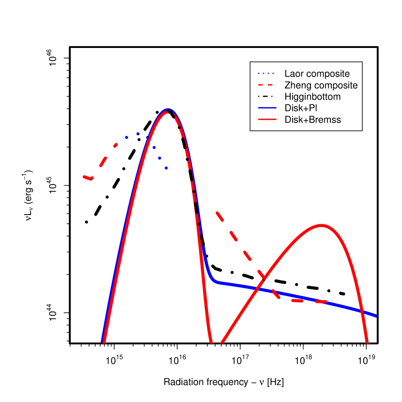
Figure 1: Multicomponent Spectral Energy Distributions (SEDs) used to calculate heating and cooling rates and radiative accelerations (SED1 (blue solid line): accretion disk + powerlaw and SED2 (red solid line): accretion disk + corona with $T_{X}=1.16\times 10^{8}$ K). We have set them as close as possible to the SEDs used in Proga & Kallman (2004) and Higginbottom et al. (2014) (black dot-dashed line), which are in turn based on Laor et al. (1997) (blue dotted line) and Zheng et al. (1997) (red dashed line) in order to facilitate comparison with previous work in the literature.

The input SEDs are shown in Fig. 1. The total luminosity is chosen to be the typical luminosity of an AGN and is based on the accretion luminosity $L_{\rm a}=2\eta GM_{BH}\dot{M}_{a}/r_{\rm Sch}$, where $\eta=0.0833$ is the accretion efficiency and $\dot{M}_{a}=1.6$ $M_{\odot}$ yr^-1 (Proga, 2007). For a fiducial SMBH with $M_{BH}=10^{8}$ $M_{\odot}$, the total luminosity is set to $L=L_{\rm a}=7.5\times 10^{45}$ erg ${\rm s}^{-1}$. The two SEDs used are multicomponent spectra similar to the ones observed for AGNs. The first one (i.e., SED1, blue solid line) is composed of an accretion disk + [X-ray]-powerlaw, while the second one (i.e., SED2, red solid line) is made of an accretion disk + [Corona]-bremsstrahlung, with $T_{X}=1.16\times 10^{8}$ K. The luminosity of the disk is defined as $L_{\rm disk}=f_{\rm disk}L$, where $f_{\rm disk}=0.95$, 0.8, and 0.5 (see Table 1), while the luminosity of the X-ray power-law is $L_{\rm pl}=f_{X}^{\rm pl}L$, with $f_{X}^{\rm pl}=0.05$, 0.2, and 0.5. The energy index of the power-law is set to $\Gamma_{\rm X}=2.1$ (with low- and high-energy cutoff equal to $10^{5}$ and $10^{10}$ K, respectively) to allow comparison with Higginbottom et al. (2014) (black dot-dashed line). The luminosity of the corona (in SED2) is set to $L_{X}=f_{X}^{c}L$, with $f_{X}^{c}=0.05$, 0.2, and 0.5. Table 1 gives a summary of the SED fractions used in the construction of the tables, and we call them calculations i, ii, iii, iv, v, and vi, respectively.

A photo-ionizing background radiation from radio to X-rays (Ostriker & Ikeuchi, 1983; Ikeuchi & Ostriker, 1986; Vedel et al., 1994) and the cosmic microwave background (CMB) have been considered, where the CMB temperature, $T_{\rm CMB}=T_{0}(1+z)$ (K), is taken to be $T_{0}=2.725\pm 0.002$ K (Mather et al., 1999; Wilkinson, 1987).

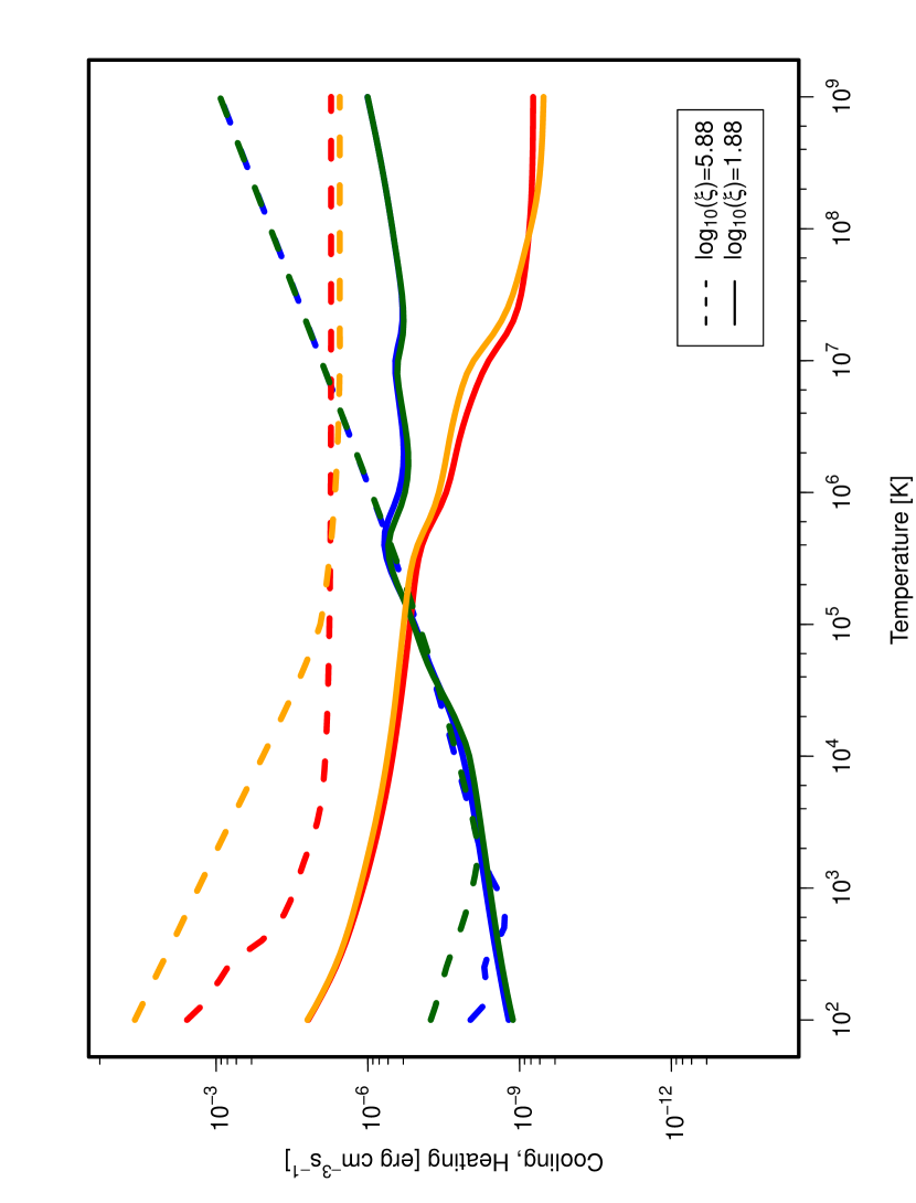
Figure 2: Cooling (blue and dark green lines) and heating (red and orange lines) rates calculated with SED1 and SED2, respectively. The solid and dashed lines correspond to ionization parameters $\log_{10}(\xi)=1.88$ and $5.88$ [ergs cm ${\rm s}^{-1}$] ($n_{H}=10^{8}$ ${\rm cm}^{-3}$), respectively. For these plots we have used $\theta=0^{\circ}$, $f_{\rm disk}=0.5$, $f^{\rm pl}_{X}=0.5$, and $f^{c}_{X}=0.5$.

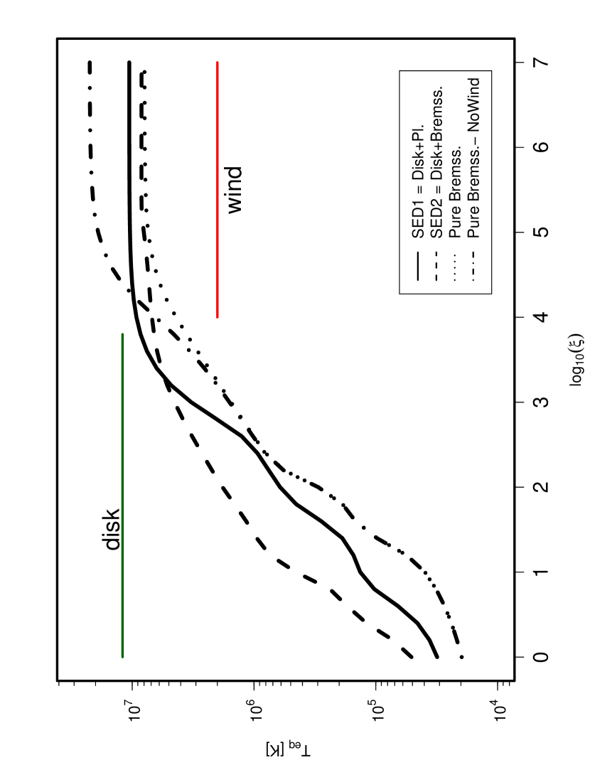
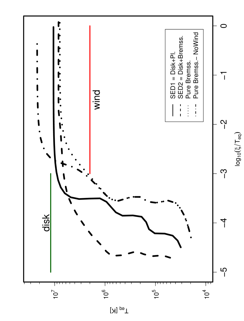
Figure 3: Gas equilibrium temperature as predicted by setting $\mathcal{H}=\mathcal{C}$ ($\rho\mathcal{L}=0$) as a function of the ionization parameter $\log_{10}(\xi)$ (top panel) and $\Xi=\log_{10}(\xi/T)$ (bottom panel), employed in models of accretion onto SMBH. The solid line shows the predictions of calculations i-iii using a disk+X-ray powerlaw. The dashed line presents calculations of disk+bremsstrahlung (SED2 as a base). The dotted and dashed-dotted lines correspond to calculations for a pure 10 keV bremsstrahlung SED with and without expansions effects. See the text for details.

A sample of the heating and cooling rates as determined from the tables is shown in Fig. 2. The gas has number density $10^{8}$ ${\rm cm}^{-3}$. In both cases, $\mathcal{C}[\rho,T]$ and $\mathcal{H}[\rho,T]$ are calculated as functions of the temperature for two different characteristic ionization parameters: $\log_{10}(\xi)=5.88$ and $1.88$ [ergs cm ${\rm s}^{-1}$]. For comparison, the blue and red lines display the total $\mathcal{C}[\rho,T]$ and $\mathcal{H}[\rho,T]$ for SED1. The dark green and orange lines display the total $\mathcal{C}[\rho,T]$ and $\mathcal{H}[\rho,T]$ for SED2. In Fig. 3, we depict the gas equilibrium temperature predicted by $\mathcal{H}=\mathcal{C}$ ($\rho\mathcal{L}=0$) as a function of the ionization parameter $\log_{10}(\xi)$ for both the heating and cooling rates calculated with the disk+corona (e.g., calculations vi, with $\theta\approx 2/5\pi$) and with the disk+X-ray powerlaw presented in calculations iii (e.g., $\theta\approx\pi/2$, see Table 1). As stated by Kallman & McCray (1982), one of the main elements of the photoionization calculations is the SED used. For instance, we have over-plotted two more calculations: one is a pure 10 keV bremsstrahlung (dotted line), which includes; a) adiabatic cooling due to the hydrodynamic expansion of the gas, ${\mathcal{C}_{\rm exp}}=-\frac{p}{\rho}\frac{{D\rho}}{{Dt}}+e\nabla\cdot{\boldsymbol{\upsilon}},$ and b) Doppler shift due to the expansion. The other is a pure 10 keV bremsstrahlung (dashed-dotted line), but in this case we have relaxed the wind model (see Eq. 2, nowind model) and as a consequence adiabatic cooling and Doppler shift effects are not taken into account. As it can be seen the net effect is to drop the equilibrium temperature of the gas from $\sim 2\times 10^{7}$ to $\sim 7\times 10^{6}$ K in the range of photoionization parameters $4\lesssim\log_{10}(\xi)\lesssim 7$.

Finally, we note an increase in $T_{\rm eq}$ in the range $0\lesssim\log_{10}(\xi)\lesssim 4$, from the nowind bremsstrahlung model to the SED2 disk+bremsstrahlung, which is basically explained by the presence of UV and hard photons that are able to photoionize the gas and contribute with the heating rate in that range of the ionization parameters. The disk-blackbody component from the accretion disc affects the lower temperature part of the stability curve (see, for example, Chakravorty et al., 2012). The nowind bremsstrahlung model curve is similar to the $T_{\rm rad}-\xi$ curve in Fig. 3 of Barai et al. (2012).

In our calculations, the net Compton heating reads as follows

$$G_{\rm comp}-\Lambda_{\rm comp}=\frac{4\pi n_{e}}{m_{e}c^{2}}\left[\int\sigma_{h}J_{\nu}\nu(1+\eta_{\nu})d\nu-4kT\int\sigma_{c}J_{\nu}d\nu\right],$$ (3)

where the Compton coefficients are $\sigma_{h}=\sigma_{T}\alpha$ and $\sigma_{c}=\sigma_{T}\alpha\beta$, with

$$\alpha=[1+\nu_{Ryd}(1.1792\times 10^{-4}+7.084\times 10^{-10}\nu_{Ryd})]^{-1},$$ (4)

and

$$\beta=[1-\alpha\nu_{Ryd}(1.1792\times 10^{-4}+1.4168\times 10^{-9}\nu_{Ryd})/4],$$ (5)

where $\nu_{Ryd}$ is the photon frequency in Rydberg. The free-free heating rate is defined as

$$G_{ff}=4\pi\int_{\nu_{c}}^{\infty}n_{e}\alpha_{\nu}(ff)J_{\nu}d\nu,$$ (6)

with $\alpha_{\nu}(ff)$ being the frequency-dependent free-free cross-section. The critical frequency $\nu_{c}$ is defined as the frequency above which the gas at a depth $r$ into the cloud becomes transparent. The free-free cooling rate is given by

$$\Lambda_{ff}=\int_{\nu_{c}}^{\infty}n_{e}\alpha_{\nu}(ff)4\pi B_{\nu}(T)d\nu,$$ (7)

where $B_{\nu}(T)$ is the frequency-dependent Planck function.

The net heating due to photoelectric and recombination cooling can be written as

$$G=G_{n,k}-\Lambda_{ind,n}-\Lambda_{spon,n},$$ (8)

where

$$G_{n,k}=n_{n}\int_{\nu_{c}}^{\infty}\frac{4\pi J_{\nu}}{h\nu}\alpha_{\nu}h(\nu-\nu_{0})d\nu,$$ (9)

while the cooling rates due to induced recombination and spontaneous radiative recombination have the form

$$\Lambda_{ind,n}=n_{e}n_{p}P^{*}_{n}\int_{\nu_{c}}^{\infty}\frac{4\pi J_{\nu}}{h\nu}\exp\left(-\frac{h\nu}{kT}\right)(\nu-\nu_{0})d\nu,$$ (10)

and

$$\Lambda_{spon,n}=n_{e}n_{p}(\frac{2\pi m_{e}k}{h^{2}})^{-3/2}\frac{8\pi}{c^{2}}\frac{g_{n}}{g_{e}g_{\rm ion}}T^{-3/2}\int_{h\nu_{0}}^{\infty}\nu^{2}\alpha_{\nu}(n)h(\nu-\nu_{0})\exp\left[-\frac{h(\nu-\nu_{0})}{kT}\right]d\nu,$$ (11)

respectively.

Finally, the net heating due to collisional ionization and cooling by 3-body recombination is defined as

$$G_{nk}-\Lambda_{nk}=\sum_{n}P^{*}_{n}n_{e}n_{p}C_{n,k}h\nu_{0}(1-b_{n}),$$ (12)

where $C_{nk}$ is the collisional ionization rate, $P^{*}$ is the LTE population, and $b_{n}$ is the departure coefficient.

The contribution from a line to the cooling rate is given by

$$\Lambda_{line}=h\nu_{ul}(n_{l}C_{lu}-n_{u}C_{ul}),$$ (13)

where $n_{u}$ and $n_{l}$ are the populations for the upper and lower levels, respectively, and the $C_{ij}$ are the collision rates. The SED1 calculated functions depicted in Fig. 2 show differences in shape and magnitude for some temperature ranges compared to those obtained using SED2.

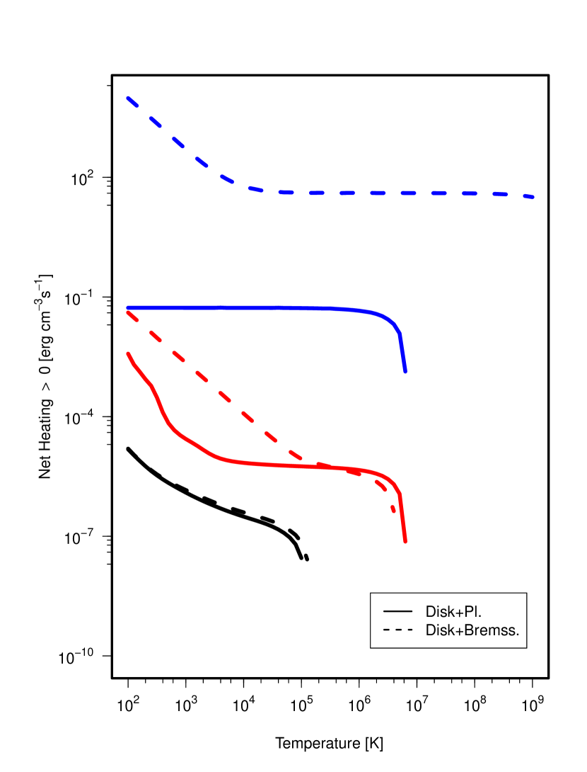
Figure 4: Net radiative heating $\rho\mathcal{L}$ as a function of temperature for the three different ionization parameters $\log_{10}(\xi)=9.88$ [ergs cm ${\rm s}^{-1}$] (blue lines), $\log_{10}(\xi)=5.88$ [ergs cm ${\rm s}^{-1}$] (red lines), and $\log_{10}(\xi)=1.88$ [ergs cm ${\rm s}^{-1}$] (black lines). The dashed lines correspond to the SED2 calculations, while the solid lines depict the net radiative heating from SED1. In both sequences of curves $n_{H}=10^{8}$ ${\rm cm}^{-3}$, $\theta=0^{\circ}$, $f_{\rm disk}=0.5$, $f^{\rm pl}_{X}=0.5$, and $f^{c}_{X}=0.5$.

Figure 4 shows the net radiative heating ($>~{}0$) of the system for three characteristic highly ionized plasmas with $\log_{10}(\xi)=9.88,5.88$, and $1.88$ [ergs cm ${\rm s}^{-1}$] (for $n_{H}=10^{8}$ ${\rm cm}^{-3}$) usually found at sub-parsec distances from the SMBH as obtained from SED2 calculations (dashed lines) and SED1 calculations (solid lines). Important differences between both net radiative heatings are observed for two of the distances tried, which may range from 50% to factors of a few percent (as expected). A higher level of the rate for all temperatures in the net heating is observed for calculations vi at $\log_{10}(\xi)=9.88$, which leads to much warmer systems at low temperatures compared to SED1’s photoionization calculations. Farther away from the BH, at ionization parameters $\log_{10}(\xi)=5.88$ and in the temperature range $10^{2}\lesssim T\lesssim 10^{4}$ the heating exhibits a steeper slope due to the removal of electrons from the pool by radiative recombination. This occurs because of the large number of available transitions at these temperatures. Nevertheless, at ionization parameters $\log_{10}(\xi)=1.88$, $\rho\mathcal{L}$ shows a very similar behavior.

3 Radiative acceleration

Along with the heating and cooling rates, we also calculate the radiative acceleration, which appears as a source term in the momentum equation

$$\rho\frac{d\boldsymbol{\upsilon}}{dt}=-\nabla p+\rho{\bf g}+\rho{\boldsymbol{\mathrm{g}}^{\rm rad}_{\rm Total}}.$$ (14)

In the tables we report here, the radiative acceleration, $\boldsymbol{\mathrm{g}}^{\rm rad}_{\rm Total}$ (defined as a force per unit mass), is calculated in a grid of $\theta$, $r$, $n_{H}$, and $T$ using cloudy 13.03. For a direct attenuated continuum, $F_{\nu}$, and a density, $\rho$, we have that

$${\boldsymbol{\mathrm{g}}^{\rm rad}_{\rm Total}}=\frac{1}{{\rho c}}\int{{F_{\nu}}{{\bar{\kappa}}_{\nu}}\;d\,\nu+}\frac{1}{{\rho c}}\sum\limits_{l}{{F_{\nu}}(l)\,{\kappa_{l}}\,{\gamma_{l}}}\;{B_{l,u}}\quad[\mathrm{cm~{}s}^{-2}],$$ (15)

where ${\bar{\kappa}}_{\nu}$ is the effective opacity from the continuum. The acceleration includes the usual photoelectric absorption as well as the free-free, Rayleigh, and Compton processes. The integral is over the range between $\lambda\approx 10$ m and $h\nu=100$ MeV. The second term is a summation over all lines contributing (typically $10^{4}$ to $10^{5}$ transitions). The quantity $\kappa_{l}$ is the opacity of the line, $B_{l,u}$ is the Einstein coefficient, and $\gamma_{l}$ is the escape probability toward the ionizing source (see Appendix B).

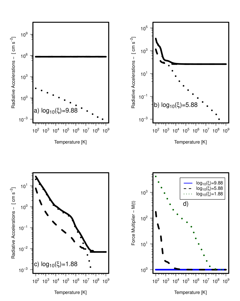
Figure 5: Calculated radiative accelerations for a BH of mass $M_{BH}=10^{8}M_{\sun}$. Panels a), b), and c) show the total outward acceleration (solid lines), the acceleration due to continuum processes (dashed lines), and that due to spectral lines (dotted lines), respectively. Panel d) shows the force multiplier (M(t)$\approx 1$: no contribution from spectral lines and M(t)$>1$: line contribution different from zero) for three characteristic ionization parameters $\log_{10}(\xi)=9.88,5.88$, and $1.88$ [ergs cm ${\rm s}^{-1}$]. In these plots we have used $\theta=0^{\circ}$, SED1, $f_{\rm disk}=0.5$, $f^{\rm pl}_{X}=0.5$, and $n_{H}=10^{8}$ ${\rm cm}^{-3}$.

In Figs. 5(a)-(c), we display the variation of the total outward acceleration (solid lines), the radiative acceleration due to continuum processes (dashed lines), and the acceleration due to spectral lines (dotted lines) with temperature for three characteristic ionization parameters: $\log_{10}(\xi)=(9.88,5.88,1.88)$ [ergs cm ${\rm s}^{-1}$]. We may see from Fig. 5(a) that in a highly ionized plasma with $\log_{10}(\xi)=9.88$ (very close to the source, $\approx 4r_{\rm Sch}$), the contribution is mostly due to scattering. At $\log_{10}(\xi)=5.88$ ($\approx 340r_{\rm Sch}$), Fig. 5(b) shows that the acceleration due to lines dominates up to $\approx 10^{3}$ K and then falls sharply at higher temperatures due to the contribution of continuum processes, while at $\log_{10}(\xi)=1.88$ ($\approx 34,000r_{\rm Sch}$), the acceleration due to spectral lines dominates over the entire range of temperatures, except for $T\gtrsim 6\times 10^{7}$ K, as shown in Fig. 5(c). The force multiplier as a function of the temperature for the above three characteristic values of $\xi$ is displayed in Fig. 5(d).

Moreover, in our calculations we assume that the contribution to $\boldsymbol{\mathrm{g}}^{\rm rad}_{\rm Total}$, coming from the disk, depends on the radial direction ($r$) and the polar angle ($\theta$) through the incident radiation

$$F_{\rm disk}(r,\theta)=\cos(\theta)\frac{L_{\rm disk}}{4\pi r^{2}},$$ (16)

while the radiative flux from the central object is isotropic

$$F_{\rm co}(r)=\frac{L_{\rm co}}{4\pi r^{2}}.$$ (17)

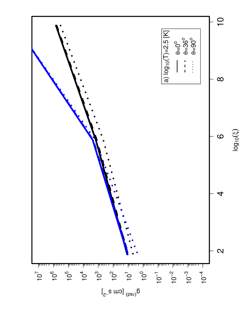
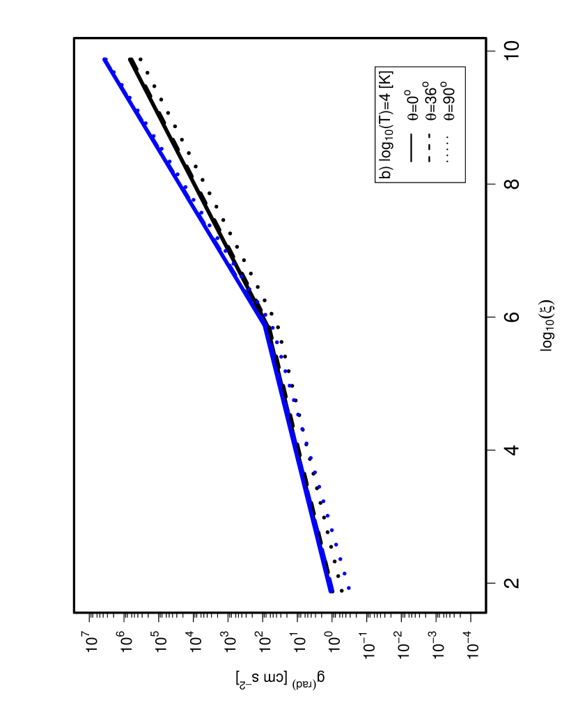
Figure 6: Total radiative force as it is usually included in the momentum equation for the simulation of accretion onto a SMBH. The black lines depict the dependence of the radiative force using calculation iii (SED1) on the ionization parameter $\xi$ for $\theta=0^{\circ}$ (solid lines), $36^{\circ}$ (dashed lines), and $90^{\circ}$ (dotted lines) as obtained from our calculations. The blue lines display the corresponding behavior as obtained using calculation vi (SED2) radiative forces. In the upper panel (a), the gas temperature is fixed to $\log_{10}T=2.5$ [K], while in the lower panel (b) $\log_{10}T=4$ [K]. When $\log_{10}T=4$ [K], differences up to a factor of $\sim 10$ are seen close to the source (distances are from $\sim 3,400r_{\rm Sch}$ to $34,000r_{\rm Sch}$).

In Fig. 6, we compare the radiative acceleration, $\boldsymbol{\mathrm{g}}^{\rm rad}_{\rm Total}$, as calculated from Eq. (15) (black lines) for SED1, with $\boldsymbol{\mathrm{g}}^{\rm rad}_{\rm Total}$, given by SED2 (blue lines), both as functions of the ionization parameter for three different angles, i.e., $\theta=$ $0^{\circ}$ (solid lines), $36^{\circ}$ (dashed lines), and $90^{\circ}$ (dotted lines). When both approaches, i.e., the calculations i-iii and the calculations iv-vi, are used in the range $0\lesssim\log_{10}(\xi)\lesssim 15$ ($10r_{\rm Sch}\lesssim r\lesssim 10,000r_{\rm Sch}$), they will both influence the distribution of velocities resulting from the momentum equation in numerical simulations of the accretion onto SMBHs.

4 The Tables

The tables are available to the public at the following links: www.abacus.cinvestav.mx/impetus and https://zenodo.org/record/58984 (catalog Zenodo). They are plain ASCII files (my1Part_OUT.txt) stored in the directories simul_$i$_$j$/, where the index $i$ corresponds to a value of the number density ($n_{H}$) and $j$ corresponds to a value of the incident angle $\theta$. For example, the sub-directory simul_$1$_$1$/ contains the ASCII text, with 12 columns (to be explained later), of the first density ($i\equiv 1$, $n_{H}=10^{-2}$ ${\rm cm}^{-3}$) and first angle ($j\equiv 1$, $\theta=0$) in our grid. Moreover, in directory simul_$101$_$6$/, one can find the calculations for $n_{H}=10^{8}$ ${\rm cm}^{-3}$ and $\theta=\pi/2$.

Each main directory is provided with an ASCII file nH_SED1_mod_11.txt, where it is easy to see the values of $i$ and $j$ corresponding to a given density and angle. Inside this file we can find:

1. Column1: Index $i$.

2. Column2: Index $j$.

3. Column3: Number density $\log_{10}(n_{H})$ [in ${\rm cm}^{-3}$].

4. Column4: Incident angle $\theta$ [in radians].

5. Column5: Initial radius $\log_{10}(r)$ [in cm].

6. Column6: Final radius $\log_{10}(r)$ [in cm].

We now describe in more detail the content of the ASCII file my1Part_OUT.txt. There are twelve (12) columns inside:

1. Column1: Incident angle $\theta$ [in radians].

2. Column2: Number density $\log_{10}(n_{H})$ [in ${\rm cm}^{-3}$].

3. Column3: Distance from the BH $\log_{10}(r)$ [in cm].

4. Column4: Temperature $\log_{10}(T)$ [in K].

5. Column5: Total cooling rate $\log_{10}(\mathcal{C})$ [in erg ${\rm cm}^{-3}$s^-1].

6. Column6: Total heating rate $\log_{10}(\mathcal{H})$ [in erg ${\rm cm}^{-3}$s^-1].

7. Column7: Acceleration due to continuum ${\boldsymbol{\mathrm{g}}^{\rm rad}_{\rm Cont}}$ [in cm s^-2].

8. Column8: Acceleration due to gravity ${\boldsymbol{\mathrm{g}}^{\rm rad}_{\rm Grav}}$ [in cm s^-2].

9. Column9: Total outward acceleration ${\boldsymbol{\mathrm{g}}^{\rm rad}_{\rm Total}}$ [in cm s^-2].

10. Column10: Acceleration due to electron scattering ${\boldsymbol{\mathrm{g}}^{\rm rad}_{\rm Elec}}$ [in cm s^-2].

11. Column11: Acceleration due to spectral lines ${\boldsymbol{\mathrm{g}}^{\rm rad}_{\rm Line}}$ [in cm s^-2].

12. Column12: Force multiplier $M_{\rm t}$ [dimensionless].

Two versions of the tables are made available: a short and a full version. The short version contains only the my1Part_OUT.txt file, the illuminating SED at $r=10^{14}$ cm (the my1contFile_OUT_14 file), and the ionic fractions at $r=10^{16}$ cm (the my1Part_OUT_frac.txt file). On average, the short version of the Tables (e.g. SED1, $f_{\rm disk}=0.95$ and $f_{X}=0.05$) occupies $\sim 47$ MB. The full version contains the full output (my1Part_OUT.out) from cloudy, which is useful to explore features related to the calculations in deeper detail. Each uncompressed directory has, on average, a size of $\sim 32$ GB. Multiplying by six this size leads to $\sim 200$ GB for the full version of the tables. A summary of the short and full versions and their location can be found in Table 2.

5 Discussion and concluding remarks

The contribution of the microphysics to the heating and cooling rates is displayed in Fig. 7. For instance, at $0.32$ pc we may see from Fig. 7(a) that the main contributor to the heating over the temperature range $400\lesssim T\lesssim 8000$ K is the Unresolved Transition Array (UTA, Behar et al. (2001); Netzer (2004) and also see Ramírez et al. (2008) for an observational point of view), which accounts for $\approx 12-16$% of the heating rate. In the interval $10^{4}\lesssim T\lesssim 8\times 10^{4}$ K, photoionization heating of O⁺⁷ becomes the major contributor, providing from $\sim 12$ to 16% of the heating. At temperatures of $10^{5}\lesssim T\lesssim 3.2\times 10^{5}$ K, Fe⁺¹⁸ contributes with $\approx 12-17$%. In these plots, the solid line labels the main contributors, while the dotted and dashed lines depict the second and third contributors, respectively. In Figs. 7(a)–(d), we see that in the temperature range $6.3\times 10^{6}\lesssim T\lesssim 3.2\times 10^{9}$ K, heating by Compton processes dominate the heating with contributions that rise up to $\approx 100$% close to the upper extreme of the temperature range.

In general, we find a rather complex interplay between the different heating agents, where low-ionization species contribute mostly at low-to-intermediate temperatures, while highly ionized species of heavy metals (e.g., Fe⁺¹⁷-Fe⁺²⁴) and intermediate heavy metals in the form of H- and He-like (e.g., O⁺⁷-O⁺⁸, C⁺⁴-C⁺⁵) become important at temperatures in the range $10^{4}\lesssim T\lesssim 10^{6}$ K. At $T\gtrsim 10^{6}$ K, Compton heating becomes the dominant mechanism. The dashed-dotted lines in Figs. 7(a)–(d) depict the contribution of the 100 main heating agents, which clearly account for $\approx 100$% of the total heating rate.

A similar analysis can be done for the cooling rate. In Fig. 8, we depict the cooling rates as a function of the temperature at different distances from the source. We see that radiative recombination cooling by H contributes to $\approx 25-74$% of the total cooling rate in the temperature range $200\lesssim T\lesssim 4\times 10^{4}$ K. Cooling by H lines dominates at higher temperatures in the interval $5\times 10^{4}\lesssim T\lesssim 4\times 10^{5}$ K with a contribution to total cooling of $\approx 25-74$%. Free-free cooling contributes with up to $\approx 86$% in the temperature interval between $\sim 1.3\times 10^{5}$ and $\sim 1.3\times 10^{8}$ K, with its contribution decreasing to $\approx 72$% at $T\sim 10^{9}$ K. The second and third contributors are represented by the dotted and dashed lines, respectively, while the dashed-dotted lines depict the contribution of the 100 main cooling agents.

Although the analytical formulas given by Blondin (1994) are useful to study cooling and heating in high-mass X-ray binary systems, they become different for simulations of gas accretion onto SMBHs in the center of galaxies, if an accretion disk emission component and an expansion model are adopted. For instance, Barai et al. (2011) discuss in detail three-dimensional SPH simulations of accretion onto a SMBH, using the heating and cooling rates proposed by Blondin (1994) (see also Mościbrodzka & Proga, 2013, for an Eulerian simulation). Some of their runs take longer to reach a steady state compared to the Bondi accretion. When analyzing radiative properties in the $T-\xi$ plane, they find many particles following the equilibrium temperature ($\mathcal{L}=0$) and discuss where and when artificial viscosity plays a dominant role over radiative heating.

Below $T=10^{4}$ K, SED1 and SED2 cooling rates differ by factors of a few. In fact, neutral-to-middle ionized gas contributes mostly to the total cooling below $T=10^{4}$ K and this can be important in the outflows ($\sim 1400$ km/s) of n iii/n iii^∗-s iii/s iii^∗ found at $\sim$ 840 pc (Chamberlain & Arav, 2015), and also in closer Iron low-ionization broad absorption lines (FeLoBAL) flows ($v\sim$ few thousands km ${\rm s}^{-1}$) at $\sim 7-70$ pc (McGraw et al., 2015). Moreover, at $\log_{10}(\xi)\sim 2$ the SED2 computations may overestimate the equilibrium temperature up to factors of $\sim 20$ in the range $10^{5}-10^{8}$ K. This may be used as a discrimination feature for simulations of SEDs in AGNs. For the heating case, however, the differences only reach factors of $\sim 2$ to $\sim 10$. We note that Compton and Coulomb heating could well be operating at temperatures between $10^{8}$ and $10^{10}$ K (for instance, in pre/post shocked winds in AGNs, Faucher-Giguère & Quataert, 2012). In addition, pure 10 keV bremsstrahlung nowind heating and cooling differ less from our calculations as the gas approaches the BH.

We further note that Vignali et al. (2015) found a gas of high velocity ($\sim 0.14$c) through the identification of highly ionized species of Iron (e.g Fe xxv and Fe xxvi) in a luminous quasar at $z\sim 1.6$ located at distances of $\sim 10^{15}$–$10^{16}$ cm. In fact, through observed high-energy features, Tombesi et al. (2015) relate low- (by molecules) and high-velocity (highly ionized gas) with the predicted energy conserved wind (Faucher-Giguère & Quataert, 2012), and locate this gas at $\sim$ 900 $r_{\rm Sch}$, where more precise estimates of the heating and cooling are required. It is therefore clear that a quantitative analysis of the heating and cooling agents operating on these kinds of astrophysical environments are key aspects towards the understanding of the radiation hydrodynamical processes governing the accretion onto SMBHs. We have provided the files my1Part_OUT.het and my1Part_OUT.col as part of the tables, where the default $\approx 10$ agents are given by cloudy. The interested reader may request the modified 100 agent files to the corresponding author.

These tables have the potential and the flexibility to include other physical effects, like dust and/or molecules. In fact, OH 119 $\mu m$ lines have been found in ultraluminous infrared galaxies (ULIRGs) using the Herschel/PACS telescope at velocities of $\sim 1000$ km ${\rm s}^{-1}$ (Veilleux et al., 2013). Also, far-ultraviolet features may be present in Mrk 231 (found with the HST), with velocities of $\sim 7000$ km ${\rm s}^{-1}$ (Veilleux et al., 2016). They permit to make more extensive exploration about the influence of the SED on photoionization calculations (see Chakravorty et al., 2009, 2012) and their impact on the energy and velocity distribution on hydrodynamical accretion processes onto SMBH. Another branch of SED to be explored are those including the reflected spectrum from the accretion disk, a rich mix of radiative recombination continua, absorption edges and fluorescent lines (García & Kallman, 2010; García et al., 2011, 2013). Additionally, if produced close to the black hole, this component suffers alterations due to relativistic effects (Dauser et al., 2013; García et al., 2014). These types of SEDs may influence cooling and heating rates as they are very sensitive to the values of the ionization parameter, temperature, and density. In astrophysical ambients like the center of AGNs, they may play an important role in high velocity winds and evolutionary stages of the host galaxies (as they may expel the cold gas reservoirs within $10^{6}-10^{8}$ years, Sturm et al., 2011). We also are in capacity to include them in tables of radiative acceleration for SPH codes, and will be the subject of a future study. A strict comparison between theoretical models and simulations is beyond the scope of the tables presented here. At present, such simulations are under preparation.

6 Acknowledgments

impetus is a collaboration project between the abacus-Centro de Matemáticas Aplicadas y Cómputo de Alto Rendimiento of Cinvestav-IPN, the Centro de Física of the Instituto Venezolano de Investigaciones Científicas (IVIC), and the Área de Física de Procesos Irreversibles of the Departamento de Ciencias Básicas of the Universidad Autónoma Metropolitana–Azcapotzalco (UAM-A) aimed at the SPH modeling of astrophysical flows. The project is supported by abacus under grant EDOMEX-2011-C01-165873, by IVIC under the project 2013000259, and by UAM-A through internal funds. JMRV thanks the hospitality, support, and computing facilities of abacus, where this work was done. We are also indebted to J. García and M. Meléndez for fruitful discussion. We want to thank the anonymous referee for providing a number of comments and suggestions that have improved both the content and style of the manuscript.

Appendix A Geometrically thin, optically thick disk used in the SEDs

The luminosity of a disk with dissipation $D(r)$ is

$$L_{\rm disk}=2\pi\int_{r_{iD}}^{\infty}D(r)rdr=\frac{1}{2}\frac{\eta GM_{BH}\dot{M}}{r_{iD}},$$ (A1)

which is half of the accretion luminosity $L_{\rm a}=\eta\dot{M}_{\rm a}c^{2}$. If the disk is optically thick and its luminosity, $L_{\rm disk}$, radiates as a blackbody, its temperature $T_{bb}(r)$ as a function of distance is given by

$$\sigma_{\rm SB}T_{bb}^{4}=\frac{1}{2}D(r),$$ (A2)

where $\sigma_{\rm SB}$ is the Stefan-Boltzmann constant and the factor $\frac{1}{2}$ enters because only one side of the disk is considered. Using the form of $D(r)$ for a viscous accretion disk, we have that

$$T_{bb}(r)=T_{\rm iD}\left(\frac{r}{r_{\rm iD}}\right)^{-3/4}\left[1-\left(\frac{r_{\rm iD}}{r}\right)^{1/2}\right]^{1/4},$$ (A3)

where

$$T_{\rm iD}=\left(\frac{3\eta GM_{BH}\dot{M}}{8\pi r_{iD}^{3}\sigma_{\rm SB}}\right)^{1/4}.$$ (A4)

For our SEDs we have used $M_{BH}=10^{8}~{}M_{\odot}$, $\dot{M}_{\rm a}=1.6~{}M_{\odot}$ yr^-1, and $r_{\rm iD}=3r_{\rm Sch}$ ($\approx r_{\rm ISCO}$ for a non-rotating SMBH). Hence, in the inner ring of the disk $T_{bb}(r_{\rm iD})=1.35\times 10^{5}$ K, while in the outer part, i.e., for $r_{\rm oD}=10r_{\rm Sch}$, the temperature would be $T_{bb}(r_{\rm oD})=4.50\times 10^{4}$ K.

Appendix B cloudy’s Ionic fractions

In our calculations we have included the following astrophysically relevant elements: H, He, C, N, O, Ne, Na, Mg, Al, Si, S, Ar, Ca, and Fe. The abundances have been taken from Grevesse et al. (2010) and we have neglected the effects of grains and molecules. Our grid of cloudy’s models for the calculation of the heating and cooling rates and the radiative acceleration uses the following physical parameters and resolutions: $\theta=0...\pi/2$ with $\Delta\theta=\pi/10$; $\log_{10}(n_{H})=-2...9$ [${\rm cm}^{-3}$] with $\Delta\log_{10}(n_{H})=0.1$; $\log_{10}(r)=14...18$ [cm] ($\approx$ 3.4 $\times$ [$1-10^{4}$] $r_{\rm Sch}$) with $\Delta\log_{10}(r)=1$; and $\log_{10}(T)=2...9$ [K] with $\Delta\log_{10}(T)=0.1$.

To look inside the cooling/heating tables we use a conventional bisection method, where for each SPH particle (or Eulerian cell) with coordinates $(r_{i},\theta_{i},\phi_{i})$ and density $\rho_{i}$, the functions $\mathcal{C}(\rho_{i},T_{i})$ and $\mathcal{H}(\rho_{i},T_{i})$ are linearly interpolated within the temperature interval $T_{\rm min}\leq T_{i}\leq T_{\rm max}$. Ferland et al. (2013) discuss in great detail the numerical algorithm and the atomic databases used by cloudy. Here we shall only describe the calculation of the level populations and refer the interested reader to Ferland et al. (2013) (and references therein) for technical details.

Radiative and collisional processes contribute to the evolution of the level populations such that

$$\frac{db_{n}}{dt}=\left.\frac{db_{n}}{dt}\right|_{\rm rad}+\left.\frac{db_{n}}{dt}\right|_{\rm col},$$ (B1)

where $b_{n}$ is the departure coefficient given by

$$b_{n}=\frac{n_{n}}{P^{*}_{n}n_{e}n_{\rm ion}},$$ (B2)

$n_{n}$ is the actual population of the level, $n_{e}$ and $n_{\rm ion}$ are, respectively, the electron and ion number density, and $P^{*}_{n}$ is the LTE relative population density for level $n$ defined as

$$P^{*}_{n}=\frac{n^{*}_{n}}{P^{*}_{n}n_{e}n_{\rm ion}}=\frac{g_{n}}{g_{e}g_{\rm ion}}\left(\frac{m^{*}_{n}}{m_{\rm ion}}\frac{h^{2}}{2\pi m_{e}kT}\right)^{3/2}\exp{\left(\frac{\chi_{n}}{kT}\right)}.$$ (B3)

Here $g_{n}=2n^{2}$ is the hydrogenic statistical weight of level $n$, $n^{*}_{n}$ is the LTE population of level $n$, $g_{e}=2$ is the electron statistical weight, $g_{\rm ion}$ is the ion statistical weight, which is equal to 1 or 2 for H- or He-like species, respectively, and $\chi_{n}$ is the ionization potential of level $n$. The other symbols are: the electron mass, $m_{e}$, the Planck constant, $h$, and the temperature, $T$.

The collisional term in Eq. (B1) can be written as

$$\begin{split}\left.\frac{db_{n}}{dt}\right|_{\rm col}=\sum_{l}b_{l}C_{nl}+\sum_{u}\frac{P^{*}_{u}}{P^{*}_{n}}b_{u}C_{un}-b_{n}\left[\sum_{l}C_{nl}+\sum_{u}\frac{P^{*}_{u}}{P^{*}_{n}}C_{un}+C_{nk}(1-b_{n}^{-1})\right],\end{split}$$ (B4)

where the summations are taken over the upper and lower levels and the $C_{ij}$ are the collisional rates in units of s^-1. The first, second, and third terms on the right-hand side of the above equation are, respectively, the collisional excitation from the lower levels to level $n$, the collisional de-excitation to level $n$ from higher levels, and the term for destruction processes. The collisional ionization rate, $C_{nk}$, is multiplied by a factor that takes into account the effects of collisional ionization and three-body recombination.

The radiative contribution term in Eq. (B1) can be written as

$$\begin{split}\left.\frac{db_{n}}{dt}\right|_{\rm rad}=\sum_{l}\frac{P^{*}_{l}}{P^{*}_{n}}b_{l}A_{nl}\frac{g_{n}}{g_{l}}\eta_{nl}\gamma_{nl}+\sum_{u}\frac{P^{*}_{u}}{P^{*}_{n}}b_{u}(A_{un}\beta_{un}+A_{un}\eta_{un}\gamma_{un})+\\ \frac{\alpha_{\rm rad}+\alpha_{\rm ind}}{P^{*}_{n}}-b_{n}\times\left[\sum_{l}(A_{nl}\beta_{nl}+A_{nl}\eta_{nl}\gamma_{nl})+\sum_{u}A_{un}\frac{g_{u}}{g_{n}}\eta_{un}\gamma_{un}+\Gamma_{n}\right],\end{split}$$ (B5)

where $A_{ij}$ is the transition probability, $\eta_{ij}\equiv J_{\nu}(ij)/(2h\nu_{ij}^{3}/c^{2})$ is the continuum occupation number of the transition $ij$, with $J_{\nu}(ij)$ being the mean intensity of the ionizing continuum at the line frequency $\nu$. The first of the two escape probabilities, $\beta$, is a two-side function, which takes into account line scattering and escape

$$\beta(\tau,T)=\frac{\beta(\tau)+\beta(\cal{T}-\tau)}{2},$$ (B6)

where $\tau$ is the optical depth of the point in question and $\cal{T}$ is the total optical depth. The escape probability, $\gamma_{ij}(\tau)$, accounts for the fraction of the primary continuum penetrating up to $\tau$ and inducing transitions between level $i$ and $j$.

The photoionization rate, $\Gamma_{n}$, from level $n$ that appears in Eq. (B5) is given by

$$\Gamma_{n}=4\pi\int_{\nu_{0}}^{\infty}\frac{J_{\nu}}{h\nu}\sigma(\nu)d\nu,$$ (B7)

and the induced recombination rate (cm³ s^-1) is defined as

$$\alpha_{{\rm ind},n}=P^{*}_{n}4\pi\int_{\nu_{0}}^{\infty}\frac{J_{\nu}}{h\nu}\sigma(\nu)\exp{\left(-\frac{h\nu}{kT}\right)}d\nu.$$ (B8)

Spontaneous radiative recombination rates, $\alpha_{\rm rad}$, are calculated as in Badnell et al. (2003) and Badnell (2006).

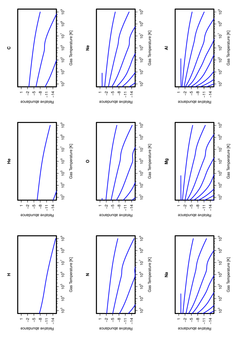
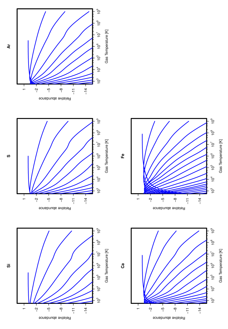
Figure 9: Relative abundances of all the elements included in our calculations (H, He, C, N, O, Ne, Na, Mg, Al, Si, S, Ar, Ca, and Fe) as a function of temperature. For these plots we have used $\theta=0^{\circ}$, SED1, $f_{\rm disk}=0.8$, $f^{\rm pl}_{X}=0.2$, and $n_{H}=10^{8}$ ${\rm cm}^{-3}$.

In summary, we have added terms which correspond to induced upward transitions from lower levels, spontaneous and induced downward transitions from higher levels, spontaneous and induced capture from the continuum to the level, and destruction of the level by radiative transitions and photoionization. The ionic emission data is taken from CHIANTI (Dere et al., 1997) and was recently revised by Landi et al. (2012). Figure 9 shows the ionic fractions for all the elements as a function of temperature. For these plots, we have chosen $n_{H}=10^{8}$ ${\rm cm}^{-3}$, $\theta=0^{\circ}$, and a distance from the source equal to $r=10^{16}$ cm (SED1, $f_{\rm disk}=0.8$, $f_{X}=0.2$).

Table 1: Emission fractions of the SEDs used for constructing the tables.

Calculation	Base SEDa	$f_{\rm disk}$	$f_{X}$	$T_{X}\times 10^{6}$ (K)b
i	1	0.95	0.05	1.79
ii	1	0.8	0.2	7.00
iii	1	0.5	0.5	18.08
iv	2	0.95	0.05	1.11
v	2	0.8	0.2	4.39
vi	2	0.5	0.5	11.87

Note. — (a) Illuminating SED used as input for a given calculation: Base SED(1)$\equiv$ Disk + Pl (Higginbottom et al., 2014); Base SED(2)$\equiv$ Disk + Bremss. (b) The Compton temperature depends on the ionization parameter which changes with density and distance with a fixed luminosity. This is $T_{X}$ for $n_{H}=10^{8}$ ${\rm cm}^{-3}$and $r=10^{16}$ cm. The entire range of $T_{X}$ for the grid of parameters that we present in these tables can be found in their large version (see Table 2).

Table 2: Table file versions and descriptions

Calc	File name	Size (MB)
i	https://zenodo.org/record/58984 (catalog New_DB_SED1_1_short.tar.gz)	36
ii	https://zenodo.org/record/58984 (catalog New_DB_SED1_2_short.tar.gz)	47
iii	https://zenodo.org/record/58984 (catalog New_DB_SED1_3_short.tar.gz)	35
iv	https://zenodo.org/record/58984 (catalog New_DB_SED2_1_short.tar.gz)	49
v	https://zenodo.org/record/58984 (catalog New_DB_SED2_2_short.tar.gz)	49
vi	https://zenodo.org/record/58984 (catalog New_DB_SED2_3_short.tar.gz)	48

Note. — The main webpage of the project is: http://www.abacus.cinvestav.mx/impetus. The full version of the tables can be accessed by from the project webpage, the links in the table above, or request to the corresponding author.

Figure 7: Main agents contributing to the heating rates as included in the tables. A complex interplay between photoelectric heating of low and high ionization species, UTA, and Compton processes can be observed. For these plots we have used a bremsstrahlung SED with $T_{X}=1.16\times 10^{8}$ K, in order to directly see the different physical mechanisms at operation for a gas with $n_{H}=10^{7}$ ${\rm cm}^{-3}$ at ionization parameters $\log(\xi)$: (a) 2.90, (b) 1.90, (c) 0.90, and (d) -0.11 [ergs cm ${\rm s}^{-1}$]. The main agents (solid lines) are also labeled by straight horizontal lines to denote the temperature range where they contribute. The second (dotted lines) and third (dashed lines) contributors are also displayed. The dotted-dashed lines correspond to the 100 main heating agents.

Figure 8: Main agents contributing to the cooling rates as included in the tables. A complex interplay between radiative and collisional recombination, collisional de-excitation of low and high ionization species, UTA, and free-free processes can be observed. For these plots we have used a bremsstrahlung SED with $T_{X}=1.16\times 10^{8}$ K, in order to directly see the different physical mechanisms at operation for a gas with $n_{H}=10^{7}$ ${\rm cm}^{-3}$ at ionization parameters $\log(\xi)$: (a) 2.90, (b) 1.90, (c) 0.90, and (d) -0.11 [ergs cm ${\rm s}^{-1}$]. The main agents (solid lines) are also labeled by straight horizontal lines to denote the temperature range where they contribute. The second (dotted lines) and third (dashed lines) contributors are also displayed. The dotted-dashed lines correspond to the 100 main cooling agents.

References

- Badnell (2006) Badnell, N. R. 2006, ApJ, 651, L73
- Badnell et al. (2003) Badnell, N. R., O’Mullane, M. G., Summers, H. P., Altun, Z., Bautista, M. A., Colgan, J., Gorczyca, T. W., Mitnik, D. M., Pindzola, M. S., & Zatsarinny, O. 2003, A&A, 406, 1151
- Barai (2008) Barai, P. 2008, ApJ, 682, L17
- Barai et al. (2011) Barai, P., Proga, D., & Nagamine, K. 2011, MNRAS, 418, 591
- Barai et al. (2012) —. 2012, MNRAS, 424, 728
- Behar et al. (2001) Behar, E., Sako, M., & Kahn, S. M. 2001, ApJ, 563, 497
- Blondin (1994) Blondin, J. M. 1994, ApJ, 435, 756
- Chakravorty et al. (2009) Chakravorty, S., Kembhavi, A. K., Elvis, M., & Ferland, G. 2009, MNRAS, 393, 83
- Chakravorty et al. (2012) Chakravorty, S., Misra, R., Elvis, M., Kembhavi, A. K., & Ferland, G. 2012, MNRAS, 422, 637
- Chamberlain & Arav (2015) Chamberlain, C. & Arav, N. 2015, MNRAS, 454, 675
- Ciotti & Ostriker (2001) Ciotti, L. & Ostriker, J. P. 2001, ApJ, 551, 131
- Dauser et al. (2013) Dauser, T., Garcia, J., Wilms, J., Böck, M., Brenneman, L. W., Falanga, M., Fukumura, K., & Reynolds, C. S. 2013, MNRAS, 430, 1694
- Dere et al. (1997) Dere, K. P., Landi, E., Mason, H. E., Monsignori Fossi, B. C., & Young, P. R. 1997, A&AS, 125, 149
- Fabian (1999) Fabian, A. C. 1999, MNRAS, 308, L39
- Faucher-Giguère & Quataert (2012) Faucher-Giguère, C.-A. & Quataert, E. 2012, MNRAS, 425, 605
- Ferland et al. (1998) Ferland, G. J., Korista, K. T., Verner, D. A., Ferguson, J. W., Kingdon, J. B., & Verner, E. M. 1998, PASP, 110, 761
- Ferland et al. (2013) Ferland, G. J., Porter, R. L., van Hoof, P. A. M., Williams, R. J. R., Abel, N. P., Lykins, M. L., Shaw, G., Henney, W. J., & Stancil, P. C. 2013, Rev. Mexicana Astron. Astrofis., 49, 137
- García et al. (2014) García, J., Dauser, T., Lohfink, A., Kallman, T. R., Steiner, J. F., McClintock, J. E., Brenneman, L., Wilms, J., Eikmann, W., Reynolds, C. S., & Tombesi, F. 2014, ApJ, 782, 76
- García et al. (2013) García, J., Dauser, T., Reynolds, C. S., Kallman, T. R., McClintock, J. E., Wilms, J., & Eikmann, W. 2013, ApJ, 768, 146
- García & Kallman (2010) García, J. & Kallman, T. R. 2010, ApJ, 718, 695
- García et al. (2011) García, J., Kallman, T. R., & Mushotzky, R. F. 2011, ApJ, 731, 131
- Gebhardt et al. (2000) Gebhardt, K., Bender, R., Bower, G., Dressler, A., Faber, S. M., Filippenko, A. V., Green, R., Grillmair, C., Ho, L. C., Kormendy, J., Lauer, T. R., Magorrian, J., Pinkney, J., Richstone, D., & Tremaine, S. 2000, ApJ, 539, L13
- Germain et al. (2009) Germain, J., Barai, P., & Martel, H. 2009, ApJ, 704, 1002
- Grevesse et al. (2010) Grevesse, N., Asplund, M., Sauval, A. J., & Scott, P. 2010, Ap&SS, 328, 179
- Higginbottom et al. (2014) Higginbottom, N., Proga, D., Knigge, C., Long, K. S., Matthews, J. H., & Sim, S. A. 2014, ApJ, 789, 19
- Ikeuchi & Ostriker (1986) Ikeuchi, S. & Ostriker, J. P. 1986, ApJ, 301, 522
- Kallman & Bautista (2001) Kallman, T. & Bautista, M. 2001, ApJS, 133, 221
- Kallman & McCray (1982) Kallman, T. R. & McCray, R. 1982, ApJS, 50, 263
- Katz et al. (1996) Katz, N., Weinberg, D. H., & Hernquist, L. 1996, ApJS, 105, 19
- Kurosawa & Proga (2009) Kurosawa, R. & Proga, D. 2009, MNRAS, 397, 1791
- Landi et al. (2012) Landi, E., Del Zanna, G., Young, P. R., Dere, K. P., & Mason, H. E. 2012, ApJ, 744, 99
- Laor et al. (1997) Laor, A., Fiore, F., Elvis, M., Wilkes, B. J., & McDowell, J. C. 1997, ApJ, 477, 93
- Li et al. (2007) Li, Y., Hernquist, L., Robertson, B., Cox, T. J., Hopkins, P. F., Springel, V., Gao, L., Di Matteo, T., Zentner, A. R., Jenkins, A., & Yoshida, N. 2007, ApJ, 665, 187
- Magorrian et al. (1998) Magorrian, J., Tremaine, S., Richstone, D., Bender, R., Bower, G., Dressler, A., Faber, S. M., Gebhardt, K., Green, R., Grillmair, C., Kormendy, J., & Lauer, T. 1998, AJ, 115, 2285
- Mather et al. (1999) Mather, J. C., Fixsen, D. J., Shafer, R. A., Mosier, C., & Wilkinson, D. T. 1999, ApJ, 512, 511
- McGraw et al. (2015) McGraw, S. M., Shields, J. C., Hamann, F. W., Capellupo, D. M., Gallagher, S. C., & Brandt, W. N. 2015, MNRAS, 453, 1379
- Mościbrodzka & Proga (2013) Mościbrodzka, M. & Proga, D. 2013, ApJ, 767, 156
- Netzer (2004) Netzer, H. 2004, ApJ, 604, 551
- Niederwanger et al. (2014) Niederwanger, F., Öttl, S., Kimeswenger, S., Kissmann, R., & Reitberger, K. 2014, in Asymmetrical Planetary Nebulae VI Conference, 67
- Novak et al. (2011) Novak, G. S., Ostriker, J. P., & Ciotti, L. 2011, ApJ, 737, 26
- Ostriker et al. (2010) Ostriker, J. P., Choi, E., Ciotti, L., Novak, G. S., & Proga, D. 2010, ApJ, 722, 642
- Ostriker & Ikeuchi (1983) Ostriker, J. P. & Ikeuchi, S. 1983, ApJ, 268, L63
- Öttl et al. (2014) Öttl, S., Kimeswenger, S., & Zijlstra, A. A. 2014, A&A, 565, A87
- Proga (2007) Proga, D. 2007, ApJ, 661, 693
- Proga & Kallman (2004) Proga, D. & Kallman, T. R. 2004, ApJ, 616, 688
- Proga et al. (2000) Proga, D., Stone, J. M., & Kallman, T. R. 2000, ApJ, 543, 686
- Ramírez et al. (2008) Ramírez, J. M., Komossa, S., Burwitz, V., & Mathur, S. 2008, ApJ, 681, 965
- Rees et al. (1989) Rees, M. J., Netzer, H., & Ferland, G. J. 1989, ApJ, 347, 640
- Salpeter (1964) Salpeter, E. E. 1964, ApJ, 140, 796
- Salz et al. (2015) Salz, M., Banerjee, R., Mignone, A., Schneider, P. C., Czesla, S., & Schmitt, J. H. M. M. 2015, A&A, 576, A21
- Sturm et al. (2011) Sturm, E., González-Alfonso, E., Veilleux, S., Fischer, J., Graciá-Carpio, J., Hailey-Dunsheath, S., Contursi, A., Poglitsch, A., Sternberg, A., Davies, R., Genzel, R., Lutz, D., Tacconi, L., Verma, A., Maiolino, R., & de Jong, J. A. 2011, ApJ, 733, L16
- Tombesi et al. (2015) Tombesi, F., Meléndez, M., Veilleux, S., Reeves, J. N., González-Alfonso, E., & Reynolds, C. S. 2015, Nature, 519, 436
- Vedel et al. (1994) Vedel, H., Hellsten, U., & Sommer-Larsen, J. 1994, MNRAS, 271, 743
- Veilleux et al. (2013) Veilleux, S., Meléndez, M., Sturm, E., Gracia-Carpio, J., Fischer, J., González-Alfonso, E., Contursi, A., Lutz, D., Poglitsch, A., Davies, R., Genzel, R., Tacconi, L., de Jong, J. A., Sternberg, A., Netzer, H., Hailey-Dunsheath, S., Verma, A., Rupke, D. S. N., Maiolino, R., Teng, S. H., & Polisensky, E. 2013, ApJ, 776, 27
- Veilleux et al. (2016) Veilleux, S., Melendez, M., Tripp, T. M., Hamann, F., & Rupke, D. S. N. 2016, ArXiv e-prints
- Vignali et al. (2015) Vignali, C., Iwasawa, K., Comastri, A., Gilli, R., Lanzuisi, G., Ranalli, P., Cappelluti, N., Mainieri, V., Georgantopoulos, I., Carrera, F. J., Fritz, J., Brusa, M., Brandt, W. N., Bauer, F. E., Fiore, F., & Tombesi, F. 2015, ArXiv e-prints
- Wilkinson (1987) Wilkinson, D. T. 1987, in Material Content of the Universe, ed. J. D. Barrow, P. J. E. Peebles, & D. W. Sciama, 163
- Zheng et al. (1997) Zheng, W., Kriss, G. A., Telfer, R. C., Grimes, J. P., & Davidsen, A. F. 1997, ApJ, 475, 469