Error estimation in the direct state tomography

Abstract

We show that reformulating the Direct State Tomography (DST) protocol in terms of projections into a set of non-orthogonal bases one can perform an accuracy analysis of DST in a similar way as in the standard projection-based reconstruction schemes. i.e. in terms of the Hilbert-Schmidt distance between estimated and true states. This allows us to determine the estimation error for any measurement strength, including the weak measurement case, and to obtain an explicit analytic form for the average minimum square errors.

I Introduction

An appealing physical idea of the weak measurement tomography johansen ; lundeen1 ; lundeen2 ; elefante ; salvail offers a possibility of reconstruction of the wave function in a single experimental setup that involves a specific system-pointer coupling; the so-called Direct State Tomography (DST). Basically, the scheme consists in successive measurements of two complementary observables of the system, where only the first one is weakly coupled to the measurement apparatus lundeen1 ; lundeen2 ; elefante ; salvail . Recently, this procedure was generalized to arbitrary coupling strengths vallone , and it was argued that the strong measurements expectably outperform the weak ones both in precision and accuracy.

Since in the framework of weak measurements the efficiency is traded for accuracy, the error estimation analysis becomes vital. Typically, the experimental performance of DST in the case of weak measurements, is compared either with results of strong (projective) tomography lundeen1 ; salvail . An alternative method of estimation of the fidelity of a reconstructed state was introduced in das . However, non of the above-mentioned approaches analyzed the global intrinsic error estimation helstrom ; englert ; checos .

In this letter we show that conveniently reformulating the approach vallone as a Mutually Unbiased Bases (MUB)-like reconstruction scheme in non-orthogonal bases pra ; jpm one can carry out the mean square error (MSE) analysis of DST , including the weak measurement limit, in the framework of measurement statistics englert ; checos . In particular, we exemplify on the single qubit case that non-orthogonal bases appear as effective projective states, in such a way that a weak coupling corresponds to projection into near-parallel bases. This allows us to reformulate the accuracy analysis in terms of measured probabilities. And thus, estimate the intrinsic statistical errors finding the minimum MSE using the Crámer-Rao lower bound.

II Direct state tomography and non-orthogonal bases

Following the general idea of DST we consider an unknown state $\rho_{s}$ of the system (one qubit) interacting with a pointer (another qubit) initially prepared in the eigenstate state $\left|0\right\rangle\left\langle 0\right|_{p}$ of the Pauli operator $\sigma_{zp}$, according to

$$U(\theta)=e^{-i\theta\sigma_{xs}\otimes\sigma_{xp}},$$

where $\theta\in[0,\pi/4]$ is the measurement strength. After the interaction the system is postselected in the state $\left|0\right\rangle_{s}$, and the pointer is measured in the bases $\{\left|\mathbf{e}^{t}\right\rangle,t=0,1,2\}$:

$$\left|e_{0}^{0}\right\rangle=\left|0\right\rangle, \left|e_{1}^{0}\right\rangle=\left|1\right\rangle,$$

$$\left|e_{0}^{1}\right\rangle=\frac{1}{\sqrt{2}}(\left|0\right\rangle+\left|1\right\rangle), \left|e_{1}^{1}\right\rangle=\frac{1}{\sqrt{2}}(\left|0\right\rangle-\left|1\right\rangle),$$

$$\left|e_{0}^{2}\right\rangle=\frac{1}{\sqrt{2}}(\left|0\right\rangle-i\left|1\right\rangle), \left|e_{1}^{2}\right\rangle=\frac{1}{\sqrt{2}}(\left|0\right\rangle+i\left|1\right\rangle),$$

and the following probabilities are retrieved

$$N_{kt}^{2}\left\langle e_{k}^{t}\right|_{p}\left\langle 0\right|_{s}U(\theta)\rho_{0}U^{{\dagger}}(\theta)\left|0\right\rangle_{s}\left|e_{k}^{t}\right\rangle_{p}=p_{kt},$$ (1)

where $\rho_{0}=\rho_{s}\otimes\left|0\right\rangle\left\langle 0\right|_{p}$ and $N_{kt}$ are the normalization constants. In the framework of DST lundeen1 , vallone the wave function is reconstructed in the basis $\{\left|e_{k}^{1}\right\rangle\}$ of eigenstates of $\sigma_{xs}$ as a linear combination of the probabilities $p_{kt}$. On the other hand, the probabilities (1) can be considered as projections of the initial state $\rho_{0}$ into the set

$$\left|\psi_{k}^{t}\right\rangle_{s}=N_{kt}\left\langle 0\right|_{p}U^{{\dagger}}(\theta)\left|0\right\rangle_{s}\left|e_{k}^{t}\right\rangle,$$ (2)

so that

$$p_{kt}=\left\langle\psi_{k}^{t}\right|\rho_{s}\left|\psi_{k}^{t}\right\rangle_{s}.$$ (3)

It is worth noticing that similar effective projection states naturally appear in experiments mdr ; shikano .

Explicitly, the effective projection states (2) have the form

$$\left|\psi_{0}^{0}\right\rangle_{s} = \left|0\right\rangle_{s},\quad\left|\psi_{1}^{0}\right\rangle_{s}=\left|1\right\rangle_{s}$$

$$\left|\psi_{k}^{1}\right\rangle_{s} = \cos\theta\left|0\right\rangle_{s}+(-1)^{k}i\sin\theta\left|1\right\rangle_{s}$$

$$\left|\psi_{k}^{2}\right\rangle_{s} = \cos\theta\left|0\right\rangle_{s}+(-1)^{k}\sin\theta\left|1\right\rangle_{s},$$ (4)

where $k=0,1$, and satisfy the condition

$$|\langle\psi_{0}^{t}|\psi_{1}^{t}\rangle|=\cos 2\theta,\;t=1,2,$$

defining the so-called equidistant bases petal .

Introducing $\lambda=\cos 2\theta$ we rewrite elements $\left|\psi_{k}^{t}\right\rangle_{s}$ as follows

$$\left|\psi_{k}^{t}(\lambda)\right\rangle_{s}=\sqrt{\frac{1+\lambda}{2}}\left|0\right\rangle_{s}+(-1)^{k}(-i)^{t+2}\sqrt{\frac{1-\lambda}{2}}\left|1\right\rangle_{s},$$ (5)

for $t=1,2$ so that $\left|\psi_{k}^{t}(\lambda=0)\right\rangle_{s}=\left|e_{k}^{t}\right\rangle$ and the limit $\lambda\rightarrow 1$ of almost “parallel” states (close to $\left|0\right\rangle$) corresponds to the weak measurement case, $\theta\rightarrow 0$.

An important feature of the probabilities $p_{kt}$, $t=1,2$ is the relation pra

$$p_{0t}+p_{1t}=1-\lambda+2\lambda p_{00}=S,$$ (6)

which reflects a statistical dependence on the measurements in the non-orthogonal and computational bases.

The bases (4) form an informationally complete set for $|\lambda|<1$ petal , and the density matrix of the system can be reconstructed in terms of the probabilities (3) according to pra

$$\rho_{s} = \frac{1}{1-\lambda^{2}}\sum_{t=1}^{2}\sum_{k=0}^{1}p_{kt}\left|\phi_{k}^{t}\right\rangle\left\langle\phi_{k}^{t}\right|$$

$$+\frac{1-\lambda}{1+\lambda}(p_{00}-1)\left|\psi_{0}^{0}\right\rangle\left\langle\psi_{0}^{0}\right|-\frac{1+\lambda}{1-\lambda}p_{00}\left|\psi_{1}^{0}\right\rangle\left\langle\psi_{1}^{0}\right|,$$

where $\left\{\left|\phi_{k}^{t}(\lambda)\right\rangle=\left|\psi_{k}^{t}(-\lambda)\right\rangle\right\}$, is the corresponding $t$-th biorthogonal basis, $\langle\phi_{k}^{t}|\psi_{l}^{t}\rangle=\sqrt{1-\lambda^{2}}\delta_{kl}$. In the limit $\lambda=0$ ($\theta=\pi/4$) the expression above is converted to the standard (orthogonal) MUB tomographic expression optimal allowing the maximum information gain wootters .

III Error estimation in direct state tomography

Each projector in the set $\{\left|\psi_{k}^{t}\right\rangle\left\langle\psi_{k}^{t}\right|,t=0,1,2;k=0,1\}$ can be considered as a single output channel of an effective measuring apparatus. An estimation procedure consists in a repetitive measurement on each of $N$ identical copies of the system, i.e. the pointer is postselected in every basis the same number of times, obtaining frequencies $\nu_{kt}=n_{kt}/N$, where $n_{kt}$ is the number of projections into $\left|\psi_{k}^{t}\right\rangle$. The corresponding statistics of outcomes is binomial-like preparacion

$$P_{t}(\mathbf{n_{t}}|\mathbf{p_{t}})=\frac{1}{S^{N}}\frac{N!}{n_{0t}!n_{1t}!}p_{0t}^{n_{0t}}p_{1t}^{n_{1t}},$$ (8)

where $\mathbf{n_{t}}=(n_{0t},n_{1t})^{T}$, $\mathbf{p_{t}}=(p_{0t}p_{1t})^{T}$, $N=n_{0t}+n_{1t}$ and the condition (6) is satisfied. For the computational basis, where $S=1$, the statistics is obviously binomial .

The expectation values corresponding to the probability distribution (8) are of the form

$$\langle n_{kt}\rangle=\frac{Np_{kt}}{S},~{}~{}\langle n_{kt}^{2}\rangle=\frac{Np_{kt}}{S^{2}}\left[(N-1)p_{kt}+S\right].$$ (9)

Following general ideas englert ; checos , we compute the estimation error as the average squared of the Hilbert-Schmidt distance between the true $\rho_{s}$ and estimated $\hat{\rho}_{s}$ system states,

$$\langle\mathcal{E}^{2}\rangle=\langle Tr[(\rho-\hat{\rho})^{2}]\rangle.$$ (10)

It depends on $\lambda$ and the inner product between all the projectors appearing in (II).

Taking into account (6) we obtain for the difference between true ($p_{kt}$) and estimated ($\hat{p}_{kt}$) probabilities, $\Delta p_{kt}=p_{kt}-\hat{p}_{kt}$, the following relations

$$\Delta p_{10} = -\Delta p_{00},$$

$$\Delta p_{1t} = 2\lambda\Delta p_{00}-\Delta p_{0t},\;t=1,2.$$

Substituting the above relations into (10) and averaging for many repetitions, we obtain for the average quadratic error

$$\left\langle\mathcal{E}^{2}\right\rangle=\sum_{t,r=0}^{2}q_{tr}\langle\Delta p_{0t}\Delta p_{0r}\rangle,$$ (11)

where the explicit form of the coefficients $q_{tr}$ (in matrix form) is given in Appendix. Employing the Cramér-Rao lower bound we minimize the possible mean square error (MSE) per trail helstrom

$$\left\langle\mathcal{E}^{2}\right\rangle\geq\operatorname{Tr}(QF^{-1}),$$ (12)

where $Q=[q_{tr}]$ and $F$ is the Fisher matrix per trail,

$$F_{tr}=\frac{1}{N}\left\langle\frac{\partial\ln\mathcal{L}}{\partial p_{0t}}\frac{\partial\ln\mathcal{L}}{\partial p_{0r}}\right\rangle,$$ (13)

being $\mathcal{L}=\prod_{i=0}^{2}P_{i}(\mathbf{n_{i}|\mathbf{p_{i}}})$ the likelihood. After straightforward but lengthy calculations (see Appendix) we find that the lower bound for the estimation error per trial in terms of measured probabilities is given by

$$\left\langle\mathcal{E}_{min}^{2}\right\rangle = \frac{2}{1-\lambda^{2}}\left[\left((1+\lambda^{2})p_{00}p_{10}+p_{01}p_{11}+p_{02}p_{12}\right)\right.$$ (14)

$$\left.-\frac{4\lambda^{2}}{S^{2}}p_{00}p_{10}\left(p_{01}p_{11}+p_{02}p_{12}\right)\right].$$

It is easy to see that at $\lambda=0$ (corresponding to $\theta=\pi/4$) the mean Hilbert-Schmidt distance for MUBs is recovered checos .

The lower bound (14) can still be averaged over the space of quantum states. We will consider pure and mixed states separately.

Let us first consider an arbitrary pure state $\left|\psi\right\rangle$ with projections $x$ and $1-x$ on the basis $\{\left|\psi_{k}^{0}\right\rangle,k=0,1\}$, that can be taken as $x=|\langle\psi|\psi_{0}^{0}\rangle|^{2}=p_{00}$ due to invariance of the averaging procedure under unitary transformations. It is straightforward to check that

$$p_{01}p_{11}+p_{02}p_{12}=\frac{S^{2}}{2}-(1-\lambda^{2})x(1-x).$$

Thus, the averaged, over the space of pure states, MSE takes the form

$$\left\langle\langle\mathcal{E}_{min}^{2}\rangle\right\rangle = \left\langle\frac{S^{2}}{1-\lambda^{2}}+\frac{8\lambda^{2}x^{2}(1-x)^{2}}{S^{2}}\right\rangle$$ (15)

$$= \frac{3+\lambda^{2}}{3(1-\lambda^{2})}+\frac{2(3-2\lambda^{2})}{3\lambda^{2}}$$

$$-\frac{2(1-\lambda^{2})}{\lambda^{3}}\operatorname{arctanh}(\lambda),$$

where the double brackets mean averaging both over the sample and over the space of states. For $\lambda=0$, corresponding to the standard MUB tomography, $\langle\langle\mathcal{E}_{min}^{2}\rangle\rangle=1$ checos , while in the limit $\lambda\rightarrow 1$ the lower bound of the MSE diverges as $\left(1-\lambda^{2}\right)^{-1}$, which qualitatively coincides with results of vallone .

In order to average over mixed states we use the eigenvalue distribution based on the Bures metric bengtsson ; hall ,

$$p(x)=\frac{2}{\pi}\frac{(1-2x)^{2}}{\sqrt{x(1-x)}}.$$

Making use of the spectral decomposition $\rho=x\left|\rho_{0}\right\rangle\left\langle\rho_{0}\right|+(1-x)\left|\rho_{1}\right\rangle\left\langle\rho_{1}\right|$, where the eigenstates can be parametrized as

$$\left|\rho_{0}\right\rangle = \cos\delta/2\left|\psi_{0}^{0}\right\rangle+e^{i\eta_{0}}\sin\delta/2\left|\psi_{1}^{0}\right\rangle$$

$$\left|\rho_{1}\right\rangle = \sin\delta/2\left|\psi_{0}^{0}\right\rangle+e^{i\eta_{1}}\cos\delta/2\left|\psi_{1}^{0}\right\rangle,$$

with $\delta\in[0,\pi]$, and $\eta_{0},\eta_{1}\in[0,2\pi]$ we perform integration of (14) with the measure $p(x)\sin\delta dxd\delta d\eta_{0}d\eta_{1}/(8\pi^{2})$. The result of such integration can be found analytically in terms of special functions and studied in the limit cases. Due to its cumbersome form we do not present the explicit expression, but instead plot it in Fig. 1.

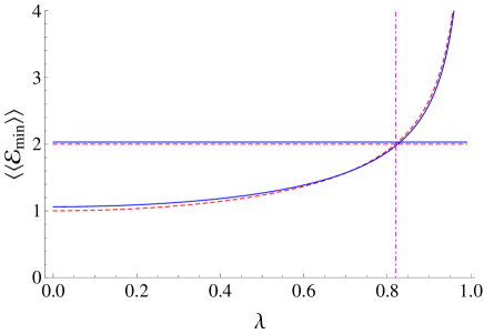
Figure 1: (Colour online) The average $\langle\langle\mathcal{E}_{min}(\lambda)\rangle\rangle$ over a sample of $10^{5}$ random statesas a fucntion of $\lambda=\cos 2\theta$: (red) dashed line for pure states, (blue) continuous line for mixed states. Average error for SIC-POVM does not depend on $\lambda$ and is represented as a constant (red) dashed line $\langle\langle\mathcal{E}_{min}\rangle\rangle=2$ for pure states and (blue) continuous line $\langle\langle\mathcal{E}_{min}\rangle\rangle=2.04$ for random mixed states. The vertical line at $\lambda=0.82$ shows the bound where the $\langle\langle\mathcal{E}_{min}(\lambda)\rangle\rangle\leq\langle\langle\mathcal{E}_{min}\rangle\rangle_{SIC-POVM}$.

In Fig. 1 we plot $\langle\langle\mathcal{E}_{min}\rangle\rangle=\sqrt{\langle\langle\mathcal{E}_{min}^{2}\rangle\rangle}$, where the average is taken for a sample of $10^{5}$ pure and mixed random states following the routine introduced in math . For pure states, the plot of the square root of equation (15) perfectly coincides with the numerical results. The mixed states are produced according to the Bures metric. As it is expected, the best estimation is obtained for MUB tomography, with $\langle\langle\mathcal{E}_{min}\rangle\rangle=1$ for pure states, and $\langle\langle\mathcal{E}_{min}\rangle\rangle\approx 1.12$ for mixed states. One can also clearly see that the stronger the measurements are, the smaller the estimation errors are.

The performance of DST can be also compared with a tomographic scheme based on symmetric informationally complete positive operator valued measure (SIC-POMV) measurements sic . For a single qubit a set of projectors $\{\Pi_{k},k=1,..,4\}$ such that $\operatorname{Tr}(\Pi_{k}\Pi_{l})=1/3,k\neq l$ and $\sum_{k=1}^{4}\Pi_{k}=I,$ span the density matrix

$$\rho_{s}=3\sum_{k=1}^{4}p_{k}\Pi_{k}-I,$$ (16)

where the probabilities $p_{k}=\operatorname{Tr}(\rho\Pi_{k})/2$ are the outcomes associated with measurement of the operator $\Pi_{k}$, $\sum_{k=1}^{4}p_{k}=1$. The corresponding MSE lower bound has the form (12), where the components of the matrix $Q$ are $q_{kl}=6\left(1+\delta_{kl}\right)$, $k,l=1,2,3$, and the Fisher matrix elements per trail are $F=1/p_{4}+\delta_{kl}/p_{k},$ which leads to $\langle\langle\mathcal{E}_{min}\rangle\rangle=2$ for pure states englert . In Fig.1 we plot $\langle\langle\mathcal{E}_{min}\rangle\rangle$ for SIC-POVM tomography as (red) dashed constant line for pure states and as a (blue) continuous constant line for mixed states, produced according to the Bures metric, obtaining in this case $\langle\langle\mathcal{E}_{min}\rangle\rangle=2.04$  by averaging over $10^{5}$ randomly generated states. One can observe that DST outperforms SIC-POVM qubit tomography for $\lambda<0.82$, which is indicated in Fig. 1 as a vertical (magenta) dotted-dashed line.

IV Conclusions

We have shown that the performance of the DST protocol can be analyzed in a similar way as in the standard projection-based reconstruction schemes. In the framework of our approach we have been able to determine the estimation error for any measurement strength, including the weak measurement case. In addition, an explicit analytic form for the minimum square error have been found in the pure and mixed states. The proposed scheme can be extended to higher dimensions and composite many-particle systems.

V Appendix: MSE lower bound for any strength measurement

In this Appendix we briefly deduce Eq. (14). Taking into account the overlaps pra

$$|\langle\phi_{k}^{i}|\phi_{l}^{i}\rangle|^{2} = (1-\lambda^{2})\delta_{k,l}+\lambda^{2},~{}~{}i=1,2$$

$$|\langle\phi_{k}^{i}|\phi_{l}^{j}\rangle|^{2} = \frac{1+\lambda^{2}}{2}~{}~{}i\neq j,k,l=0,1$$

$$|\langle\phi_{0}^{0}|\phi_{l}^{i}\rangle|^{2} = \frac{1-\lambda}{2}~{}~{}i,j=1,2,k,l=0,1$$

$$|\langle\phi_{1}^{0}|\phi_{l}^{i}\rangle|^{2} = \frac{1+\lambda}{2}~{}~{}i,j=1,2,k,l=0,1,$$

and substituting the restrictions $\Delta p_{10}=-\Delta p_{00}$, $\Delta p_{1i}=2\lambda\Delta p_{00}-\Delta p_{0i}$ into (10) and (II) one arrives to

$$Q=\frac{2}{1-\lambda^{2}}\left(\begin{array}[]{ccc}1+\lambda^{2}&-\lambda&-\lambda\\ -\lambda&1&0\\ -\lambda&0&1\end{array}\right).$$

The Fisher matrix (per trial) (13) is obtained directly form the likelihood

$$\mathcal{L}=\frac{1}{S^{2N}}\prod_{i=0}^{2}\frac{N!}{n_{0i}!n_{1i}!}p_{0i}^{n_{0i}}p_{1i}^{n_{1i}}.$$

In particular, one has

$$F_{00}=\frac{1}{p_{00}}+\frac{1}{p_{10}}+\frac{4\lambda^{2}}{S}\left(\frac{1}{p_{11}}+\frac{1}{p_{12}}\right)-\frac{8\lambda^{2}}{S^{2}},$$

where the two first terms correspond to the MUB tomography checos , the third term appears due to dependence of the sum of probabilities in the non-orthogonal bases on $p_{00}$, and the last term comes form the normalization factor $S^{-2N}$. The main difference with the MUB case consists in appearing elements in $F$ outside of the main diagonal, which is a consequence of the relation (6):

$$F_{0t}=F_{t0}=-\frac{2\lambda}{Sp_{1t}},~{}~{}t=1,2$$

For the non-orthogonal bases $t,r=1,2$, the elements are similar to the MUB case, normalized by the factor $S$:

$$F_{tr}=\frac{1}{S}\left(\frac{1}{p_{0t}}+\frac{1}{p_{1t}}\right)\delta_{tr}.$$

Substituting the explicit forms of $Q$ and $F$ into (12) one obtains (14).

References

• (1) L. M. Johansen, Phys. Rev. A 76, 012119 (2007).
• (2) J. S. Lundeen, B. Sutherland, A. Patel, C. Stewart, and C. Bamber, Nature 474, 188 (2011).
• (3) J. S. Lundeen and C. Bamber, Phys. Rev. Lett. 108, 070402 (2012).
• (4) S. Wu, Scientific Reports 3, 1193 (2013).
• (5) J. Z. Salvail, M. Agnew, A. S. Johnson, E. Bolduc, J. Leach, and R. W. Boyd, Nature Photonics 7, 316-321 (2013).
• (6) G. Vallone and D. Dequal, Phys. Rev. Lett. 116, 040502 (2016).
• (7) D. Das, and Arvind, Phys. Rev. A 89, 062121 (2014).
• (8) H. Zhu and B.-G. Englert, Phys. Rev. A 84, 022327 (2011).
• (9) J. Řeháček, Z. Hradil, A.B. Klimov, G. Leuchs, and L.L. Sánchez-Soto, Phys. Rev A 88, 052110 (2013).
• (10) C.W. Helstrom, Quantum detection and estimation theory (Academic Press, 1976).
• (11) I. Sainz, L. Roa, and A. B. Klimov, Phys. Rev. A 81, 052114 (2010).
• (12) I. Sainz, L. Roa, and A. B. Klimov, J. Math. Phys. 53, 052102 (2012).
• (13) J. Erhart, et al, Nat. Phys. 8, 185 (2012); L.A. Rozema, et al, Phys. Rev. Lett. 109, 100404 (2012); S.-Y. Baek, et al, Sci. Rep. 3, 2221 (2013); M. Ringbauer, et al, Phys. Rev. Lett. 112, 020401 (2014).
• (14) H. Kobayashi, k. Nonaka, and Y. Shikano, Phys. Rev. A 89, 053816 (2014).
• (15) L. Roa, C. Hermann-Avigliano, R. Salazar, and A. B. Klimov, Phys. Rev. A 84, 014302 (2011).
• (16) I. D. Ivanovic, J. Phys. A 13, 3241 (1981); W. K. Wootters, Annals of Physics 176, 1 (1988).
• (17) W.K. Wootters and B. D. Fields, Annals of Physics 191, 363 (1989).
• (18) I. Sainz, A.B. Klimov, and L. Roa, Phys. Rev. A 88, 033819 (2013).
• (19) I. Bengtsson and K. Życkowski, Geometry of quantum states, Cambridge University Press (2008).
• (20) M. J. W. Hall, Phys. Lett. A 242, 123 (1998).
• (21) J.A. Miszczak, Int. J. Mod. Phys. C 22, 897-918 (2011); J.A. Miszczak, Z. Puchala, and P. Gawron, QI: quantum information package for Mathematica, http://zksi.iitis.pl/wiki/projects:mathematica-qi (2010).
• (22) G. M. D’Ariano, M. G. A. Paris, and M. F. Sacchi, Quantum Tomography, in Advances in Imagin and Electronics Physics 128 (Academic Press, 2003).