Focused Model-Learning and Planning for
Non-Gaussian Continuous State-Action Systems

Abstract\\

We introduce a framework for model learning and planning in stochastic domains with continuous state and action spaces and non-Gaussian transition models. It is efficient because (1) local models are estimated only when the planner requires them; (2) the planner focuses on the most relevant states to the current planning problem; and (3) the planner focuses on the most informative and/or high-value actions. Our theoretical analysis shows the validity and asymptotic optimality of the proposed approach. Empirically, we demonstrate the effectiveness of our algorithm on a simulated multi-modal pushing problem.

1 Introduction

Most real-world domains are sufficiently complex that it is difficult to build an accurate deterministic model of the effects of actions. Even with highly accurate actuators and sensors, stochasticity still widely appears in basic manipulations, especially non-prehensile ones [36]. The stochasticity may come from inaccurate execution of actions as well as from lack of detailed information about the underlying world state. For example, rolling a die is a deterministic process that depends on the forces applied, air resistance, etc.; however, we are not able to model the situation sufficiently accurately to plan reliable actions, nor to execute them repeatably if we could plan them. We can plan using a stochastic model of the system, but in many situations, such as rolling dice or pushing a can shown in Fig. 1, the stochasticity is not modeled well by additive single-mode Gaussian noise, and a more sophisticated model class is necessary.

In this paper, we address the problem of learning and planning for non-Gaussian stochastic systems in the practical setting of continuous state and action spaces. Our framework learns transition models that can be used for planning to achieve different objectives in the same domain, as well as to be potentially transferred to related domains or even different types of robots. This strategy is in contrast to most reinforcement-learning approaches, which build the objective into the structure being learned. In addition, rather than constructing a single monolithic model of the entire domain which could be difficult to represent, our method uses a memory-based learning scheme, and computes localized models on the fly, only when the planner requires them. To avoid constructing models that do not contribute to improving the policy, the planner should focus only on states relevant to the current planning problem, and actions that can lead to high reward.

We propose a closed-loop planning algorithm that applies to stochastic continuous state-action systems with arbitrary transition models. It is assumed that the transition models are represented by a function that may be expensive to evaluate. Via two important steps, we focus the computation on the current problem instance, defined by the starting state and goal region. To focus on relevant states, we use real time dynamic programming (RTDP) [2] on a set of states strategically sampled by a rapidly-exploring random tree (RRT) [18, 13]. To focus selection of actions from a continuous space, we develop a new batch Bayesian optimization (BO) technique that selects and tests, in parallel, action candidates that will lead most quickly to a near-optimal answer.

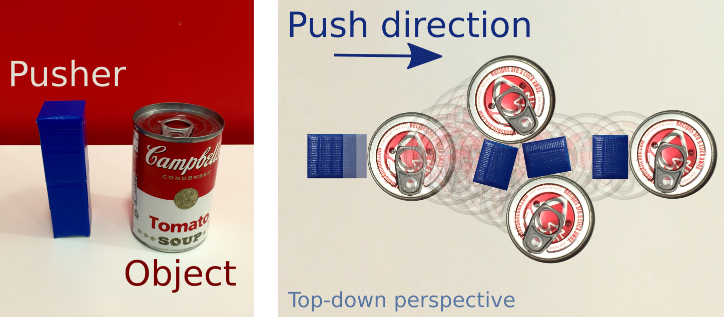
Figure 1: A quasi-static pushing problem: the pusher has a velocity controller with low gain, resulting in non-Gaussian transitions. We show trajectories for object and pusher resulting from the same push velocity.

We show theoretically that the expected accumulated difference between the optimal value function of the original problem and the value of the policy we compute vanishes sub-linearly in the number of actions we test, under mild assumptions. Finally we evaluate our approach empirically on a simulated multi-modal pushing problem, and demonstrate the effectiveness and efficiency of the proposed algorithm.

2 Related Work

Learning

The class of problems that we address may be viewed as reinforcement-learning (RL) problems in observable continuous state-action spaces. It is possible to address the problem through model-free RL, which estimates a value function or policy for a specific goal directly through experience. Though the majority of work in RL addresses domains with discrete action spaces, there has been a thread of relevant work on value-function-based RL in continuous action spaces [12, 1, 24, 31, 23]. An alternative approach is to do direct search in the space of policies [6, 14].

In continuous state-action spaces, model-based RL, where a model is estimated to optimize a policy, can often be more effective. Gaussian processes (GP) can help to learn the dynamics [7, 26, 22], which can then be used by GP-based dynamic programming [8, 26] to determine a continuous-valued closed-loop policy for the whole state space. More details can be found in the excellent survey [10].

Unfortunately, the common assumption of i.i.d Gaussian noise on the dynamics is restrictive and may not hold in practice [36], and the transition model can be multi-modal. It may additionally be difficult to obtain a good GP prior. The basic GP model is can capture neither the multi-modality nor the heteroscedasticity of the noise. While more advanced GP algorithms may address these problems, they often suffer from high computational cost [29, 37].

Moldovan et al. [21] addressed the problem of multi-modality by using Dirichlet process mixture models (DPMMs) to learn the density of the transition models. Their strategies for planning were limited by deterministic assumptions, appropriate for their domains of application, but potentially resulting in collisions in ours. Kopicki et al. [16, 15, 17] addressed the problem of learning to predict the behavior of rigid objects under manipulations such as pushing, using kernel density estimation. In this paper, we propose an efficient planner that can work with arbitrary, especially multi-modal stochastic models in continuous state-action spaces. Our learning method in the experiment resembles DPMMs but we estimate the density on the fly when the planner queries a state-action pair. We were not able to compare our approach with DPMMs because we found DPMMs not computationally feasible for large datasets.

Planning

We are interested in domains for which queries are made by specifying a starting state and a goal set, and in which the solution to the given query can be described by a policy that covers only a small fraction of the state space that the robot is likely to encounter.

Planning only in the fraction of the state-action space that the robot is likely to encounter is, in general, very challenging. Other related work uses tree-based search methods [33, 19, 35], where the actions are selected by optimizing an optimistic heuristic. These algorithms are impractical for our problem because of the exponential growth of the tree and the lack of immediate rewards that can guide the pruning of the tree.

In contrast to the tree-search algorithms, iMDP [13], which is most related to our work, uses sampling techniques from RRTs to create successively more accurate discrete MDP approximations of the original continuous MDP, ultimately converging to the optimal solution to the original problem. Their method assumes the ability to solve the Bellman equation optimally (e.g. for a simple stochastic LQR problem), the availability of the backward transition models, and that the dynamics is modeled by a Wiener process, in which the transition noise is Gaussian with execution-time-dependent variance. However, the assumptions are too restrictive to model our domains of interest where the dynamics is non-closed-form, costly to evaluate, non-reversible, and non-Gaussian. Furthermore, iMDP is designed for stochastic control problems with multiple starting states and a single goal, while we are interested in multiple start-goal pairs.

Our work builds on the idea of constructing a sequence of MDPs from iMDP [13], and aims at practically resolving the challenges of state/action selection faced by both iMDP and tree-search-based planners [33].

Bayesian optimization

There have been a number of applications of BO in optimal control, although to our knowledge, it has not been previously applied to action-selection in continuous-action MDPs. BO has been used to find weights in a neural network controller [9], to solve for the parameters of a hierarchical MDP [3], and to address safe exploration in finite MDPs [30]. To our knowledge, BO has not been previously applied to action-selection in continuous-action MDPs.

3 Problem formulation

Let the state space $S\subset\mathbb{R}^{d_{s}}$ with metric $d$ and the control space $U\subset\mathbb{R}^{d_{u}}$ both be compact and measurable sets. The interior of the state space $S$ is $S^{o}$ and the boundary is $\partial S$. For the control space $U$, there exists an open set $U^{o}$ in $R^{d_{u}}$ such that $U$ is the closure of $U^{o}$. We assume the state is fully observed (any remaining latent state will manifest as stochasticity in the transition models). Actions $a=(u,\Delta t)$ are composed of both a control on the robot and the duration for which it will be exerted, so the action space is $A=U\times[T_{min},T_{max}]$, where $T_{min},T_{max}\in\mathbb{R}_{+}\setminus\{\infty\}$ are the minimum and the maximum amount of duration allowed. The action space $A$ is also a compact set. The starting state is $s_{0}$, and the goal region is denoted as $\mathcal{G}\subset S$, in which all states are terminal states. We assume $\mathcal{G}$ has non-zero measure, and $S$ has finite measure. The transition model has the form of a continuous probability density function $p_{s^{\prime}\mid s,a}$ on the resulting state $s^{\prime}$, given previous state $s$ and action $a$, such that $\forall s^{\prime}\in S,p_{s^{\prime}\mid s,a}(s^{\prime}\mid s,a)\geq 0,\int_{S}p(s^{\prime}\mid s,a)\mathop{}\!\mathrm{d}s^{\prime}=1$.

Given a transition model and a cost function $C:S\times S\times A\rightarrow\mathbb{R}$ associated with a goal region, we can formulate the problem as a continuous state-action MDP $(S,A,p_{s^{\prime}\mid s,a},R,\gamma)$, where $R(s^{\prime}\mid s,a)=-C(s^{\prime}\mid s,a)$ is the immediate reward function and $\gamma$ is the discount factor. A high reward is assigned to the states in the goal region $\mathcal{G}$, and a cost is assigned to colliding with obstacles or taking any action. We would like to solve for the optimal policy $\pi:S\rightarrow A$, for which the value of each state $s$ is

$$V^{\pi}(s)=\underset{a\in A}{\max}\int_{s^{\prime}\in S}p_{s^{\prime}\mid s,a}(s^{\prime}\mid s,a)\left(R(s^{\prime}\mid s,a)+\gamma^{\Delta t}V^{\pi}(s^{\prime})\right)\mathop{}\!\mathrm{d}s^{\prime}.$$

4 Our method: BOIDP

We describe our algorithm Bayesian Optimization Incremental-realtime Dynamic Programming (BOIDP) in this section. At the highest level, BOIDP in Alg. 1 operates in a loop, in which it samples a discrete set of states $\tilde{S}\subset S$ and attempts to solve the discrete-state, continuous-action MDP $\tilde{\mathcal{M}}=(\tilde{S},A,\hat{P}_{s^{\prime}\mid s,a},R,\gamma)$. Here $\hat{P}_{s^{\prime}\mid s,a}(s^{\prime}\mid s,a)$ is the probability mass function for the transition from state $s\in\tilde{S}$ and action $a\in A$ to a new state $s^{\prime}\in\tilde{S}$. The value function for the optimal policy of the approximated MDP $\tilde{\mathcal{M}}$ is $V(s)=\underset{a\in A}{\max}\;Q_{s}(a),$ where

$$Q_{s}(a)=\sum_{s^{\prime}\in\tilde{S}}\hat{P}_{s^{\prime}\mid s,a}(s^{\prime}\mid s,a)\left(R(s^{\prime}\mid s,a)+\gamma^{\Delta t}V(s^{\prime})\right).$$ (1)

If the value of the resulting policy is satisfactory according to the task-related stopping criterion, we can proceed; otherwise, additional state samples are added and the process is repeated. Once we have a policy $\pi$ on $\tilde{S}$ from RTDP, the robot can iteratively obtain and execute the policy for the nearest state to the current state in the sampled set $\tilde{S}$ by the metric $d$.

There are a number of challenges underlying each step of BOIDP. First, we need to find a way of accessing the transition probability density function $p_{s^{\prime}\mid s,a}$ , which is critical for the approximation of $\hat{P}_{s^{\prime}\mid s,a}(s^{\prime}\mid s,a)$ and the value function. We describe our “lazy access” strategy in Sec. 4.1. Second, we must find a way to compute the values of as few states as possible to fully exploit the “lazy access” to the transition model. Our solution is to first use an RRT-like process [18, 13] to generate the set of states that asymptotically cover the state space with low dispersion (Sec. 4.2), and then “prune” the irrelevant states via RTDP [2] (Sec. 4.3). Last, each dynamic-programming update in RTDP requires a maximization over the action space; we cannot achieve this analytically and so must sample a finite set of possible actions. We develop a new batch BO algorithm to focus action sampling on regions of the action space that are informative and/or likely to be high-value, as described in Sec. 4.4.

Both the state sampling and transition estimation processes assume a collision checker $\textsc{ExistsCollision}(s,a,s^{\prime})$ that checks the path from $s$ to $s^{\prime}$ induced by action $a$ for collisions with permanent objects in the map.

Algorithm 1 BOIDP

1:function BOIDP($s_{0},\mathcal{G},S,p_{s^{\prime}\mid s,a},N_{\min}$)

2:    $\tilde{S}\leftarrow\{s_{0}\}$

3:    loop

4:         $\tilde{S}\leftarrow\textsc{SampleStates}(N_{\min},\tilde{S},\mathcal{G},S,p_{s^{\prime}\mid s,a})$

5:         $\pi,V=\textsc{RTDP}(s_{0},\mathcal{G},\tilde{S},p_{s^{\prime}\mid s,a})$     

6:    until stopping criteria reached

7:    ExecutePolicy($\pi,\tilde{S},\mathcal{G}$)

8:

9:function ExecutePolicy($\pi,\tilde{S},\mathcal{G}$)

10:    loop

11:         $s_{c}\leftarrow$ current state

12:         $\tilde{s}\leftarrow\operatorname{arg\,min}_{s\in\tilde{S}}d(s,s_{c})$

13:         Execute $\pi(\tilde{s})$     

14:    until current state is in $\mathcal{G}$

4.1 Estimating transition models in BOIDP

In a typical model-based learning approach, first a monolithic model is estimated from the data and then that model is used to construct a policy. Here, however, we aim to scale to large spaces with non-Gaussian dynamics, a setting where it is very difficult to represent and estimate a single monolithic model. Hence, we take a different approach via “lazy access” to the model: we estimate local models on demand, as the planning process requires information about relevant states and actions.

Algorithm 2 Transition model for discrete states

1:function TransitionModel($s,a,\tilde{S},p_{s^{\prime}\mid s,a}$)

2:    $\hat{S}\leftarrow\textsc{HighProbNextStates}(p_{s^{\prime}\mid s,a}(\tilde{S}\mid s,a))\cup\{s_{obs}\}$ $\triangleright$ $s_{obs}$ is a terminal state

3:    $\hat{P}_{s^{\prime}\mid s,a}(\hat{S}\mid s,a)\leftarrow p_{s^{\prime}\mid s,a}(\hat{S}\mid s,a)$

4:    for $s^{\prime}$ in $\hat{S}$ do

5:         if $s^{\prime}\in S^{o}$ and ExistsCollision($s,a,s^{\prime}$) then

6:             $\hat{P}_{s^{\prime}\mid s,a}(s_{obs}\mid s,a)\leftarrow\hat{P}_{s^{\prime}\mid s,a}(s_{obs}\mid s,a)+\hat{P}_{s^{\prime}\mid s,a}(s^{\prime}\mid s,a)$

7:             $\hat{P}_{s^{\prime}\mid s,a}(s^{\prime}\mid s,a)\leftarrow 0$              

8:    $\hat{P}_{s^{\prime}\mid s,a}(\hat{S}\mid s,a)\leftarrow\textsc{Normalize}(\hat{P}_{s^{\prime}\mid s,a}(\hat{S}\mid s,a))$

9:    return $\hat{S},\hat{P}_{s^{\prime}\mid s,a}(\hat{S}\mid s,a)$

We assume a dataset $D=\{s_{i},a_{i},s^{\prime}_{i}\}_{i=0}^{N}$ for the system dynamics and the dataset is large enough to provide a good approximation to the probability density of the next state given any state-action pair. If a stochastic simulator exists for the transition model, one may collect the dataset dynamically in response to queries from BOIDP. The “lazy access” provides a flexible interface, which can accommodate a variety of different density-estimation algorithms with asymptotic theoretical guarantees, such as kernel density estimators [34] and Gaussian mixture models [20]. In our experiments, we focus on learning Gaussian mixture models with the assumption that $p_{s^{\prime}\mid s,a}(s^{\prime}\mid s,a)$ is distributed according to a mixture of Gaussians $\forall(s,a)\in S\times A$.

Given a discrete set of states $\tilde{S}$, starting state $s$ and action $a$, we compute the approximate discrete transition model $\hat{P}_{s^{\prime}\mid s,a}$ as shown in Algorithm 2. We use the function HighProbNextStates to select the largest set of next states $\hat{S}\subseteq\tilde{S}$ such that $\forall s^{\prime}\in\hat{S},p_{s^{\prime}\mid s,a}(s^{\prime}\mid s,a)>\epsilon$. $\epsilon$ is a small threshold parameter, e.g. we can set $\epsilon=10^{-5}$. If $p_{s^{\prime}\mid s,a}$ does not take obstacles into account, we have to check the path from state $s$ to next state $s^{\prime}\in\tilde{S}$ induced by action $a$ for collisions, and model their effect in the approximate discrete transition model $\hat{P}_{s^{\prime}\mid s,a}$. To achieve this, we add a dummy terminal state $s_{obs}$, which represents a collision, to the selected next-state set $\hat{S}$. Then, for any $s,a,s^{\prime}$ transition that generates a collision, we move the probability mass $\hat{P}_{s^{\prime}\mid s,a}(s^{\prime}\mid s,a)$ to the transition to the collision state $\hat{P}_{s^{\prime}\mid s,a}(s_{obs}\mid s,a)$. Finally, $\hat{P}_{s^{\prime}\mid s,a}(\hat{S}\mid s,a)$ is normalized and returned together with the selected set $\hat{S}$.

These approximated discrete transition models can be indexed by state $s$ and action $a$ and cached for future use in tasks that use the same set of states $\tilde{S}$ and the same obstacle map. The memory-based essence of our modeling strategy is similar to the strategy of non-parametric models such as Gaussian processes, which make predictions for new inputs via smoothness assumptions and similarity between the query point and training points in the data set.

For the case where the dynamics model $p_{s^{\prime}\mid s,a}$ is given, computing the approximated transition $\hat{P}_{s^{\prime}\mid s,a}$ could still be computationally expensive because of the collision checking. Our planner is designed to alleviate the high computation in $\hat{P}_{s^{\prime}\mid s,a}$ by focusing on the relevant states and actions, as detailed in the next sections.

4.2 Sampling states

Algorithm 3 describes the state sampling procedures. The input to SampleStates in Alg. 3 includes the minimum number of states, $N_{\min}$, to sample at each iteration of BOIDP. It may be that more than $N_{\min}$ states are sampled, because sampling must continue until at least one terminal goal state is included in the resulting set $\tilde{S}$. To generate a discrete state set, we sample states both in the interior of $S^{o}$ and on its boundary $\partial S$. Notice that we can always add more states by calling SampleStates.

Algorithm 3 RRT states sampling for BOIDP

1:function SampleStates($N_{min},\tilde{S},\mathcal{G},S,p_{s^{\prime}\mid s,a}$)

2:    $\tilde{S}^{o}\leftarrow\textsc{SampleInteriorStates}(\lceil N_{min}/2\rceil,\tilde{S},\mathcal{G},S,p_{s^{\prime}\mid s,a})$

3:    $\partial\tilde{S}\leftarrow\textsc{SampleBoundaryStates}(\lceil N_{min}/2\rceil,\tilde{S},\mathcal{G},S,p_{s^{\prime}\mid s,a})$

4:    return $\tilde{S}^{o}\cup\partial\tilde{S}$

5:

6:function SampleInteriorStates($N_{min},\tilde{S},\mathcal{G},S,p_{s^{\prime}\mid s,a}$)

7:    while $\mid\tilde{S}\mid<N_{min}$ or $\mathcal{G}\cap\tilde{S}=\emptyset$ do

8:         $s_{rand}\leftarrow\textsc{UniformSample}(S)$

9:         $s_{nearest}\leftarrow\textsc{Nearest}(s_{rand},\tilde{S})$

10:         $s_{n},a_{n}\leftarrow\textsc{RRTExtend}(s_{nearest},s_{rand},p_{s^{\prime}\mid s,a})$

11:         if found $s_{n},a_{n}$ then

12:             $\tilde{S}\leftarrow\tilde{S}\cup\{s_{n}\}$              

13:    return $\tilde{S}$

14:

15:function RRTExtend($s_{nearest},s_{rand},p_{s^{\prime}\mid s,a}$)

16:    $d_{n}=\infty$

17:    while stopping criterion not reached do

18:         $a\leftarrow\textsc{UniformSample}(A)$

19:         $s^{\prime}\leftarrow\textsc{Sample}\left(p_{s^{\prime}\mid s,a}(\cdot\mid s_{nearest},a)\right)$

20:         if  $\left(\textbf{not }\textsc{ExistsCollision}(s,s^{\prime},a)\right)$ and $d_{n}>d(s_{rand},s^{\prime})$ then

21:             $d_{n}\leftarrow d(s_{rand},s^{\prime})$

22:             $s_{n},a_{n}\leftarrow s^{\prime},a$              

23:    return $s_{n},a_{n}$

To generate one interior state sample, we randomly generate a state $s_{rand}$, and find $s_{nearest}$ that is the nearest state to $s_{rand}$ in the current sampled state set $\tilde{S}$. Then we sample a set of actions from $A$, for each of which we sample the next state $s_{n}$ from the dataset $D$ given the state-action pair $s_{neareast},a$ (or from $p_{s^{\prime}\mid s,a}$ if given). We choose the action $a$ that gives us the $s_{n}$ that is the closest to $s_{rand}$. To sample states on the boundary $\partial S$, we assume a uniform random generator for states on $\partial S$ is available. If not, we can use something similar to SampleInteriorStates but only sample inside the obstacles uniformly in line 8 of Algorithm 3. Once we have a sample $s_{rand}$ in the obstacle, we try to reach $s_{rand}$ by moving along the path $s_{rand}\rightarrow s_{n}$ incrementally until a collision is reached.

4.3 Focusing on the relevant states via RTDP

We apply our algorithm with a known starting state $s_{0}$ and goal region $\mathcal{G}$. Hence, it is not necessary to compute a complete policy, and so we can use RTDP [2] to compute a value function focusing on the relevant state space and a policy that, with high probability, will reach the goal before it reaches a state for which an action has not been determined. We assume an upper bound of the values for each state $s$ to be $h_{u}(s)$. One can approximate $h_{u}(s)$ via the shortest distance from each state to the goal region on the fully connected graph with vertices $\tilde{S}$. We show the pseudocode in Algorithm 4.

Algorithm 4 RTDP for BOIDP

1:function RTDP($s_{0},\mathcal{G},\tilde{S},p_{s^{\prime}|s,a}$)

2:    for $s$ in $\tilde{S}$ do

3:         $V(s)=h_{u}(s)$ $\triangleright$ Compute the value upper bound     

4:    while $V(\cdot)$ not converged do

5:         $\pi,V\leftarrow\textsc{TrialRecurse}(s_{0},\mathcal{G},\tilde{S},p_{s^{\prime}|s,a})$     

6:    return $\pi,V$

7:

8:function TrialRecurse($s,\mathcal{G},\tilde{S},p_{s^{\prime}|s,a}$)

9:    if reached cycle or $s\in\mathcal{G}$  then

10:         return     

11:    $\pi(s)\leftarrow\operatorname{arg\,max}_{a}Q(s,a,\tilde{S},p_{s^{\prime}|s,a})$ $\triangleright$ Max via BO

12:    $s^{\prime}\leftarrow\textsc{Sample}(\hat{P}_{s^{\prime}|s,a}(\tilde{S}|s,\pi(s)))$

13:    $\textsc{TrialRecurse}(s^{\prime},\mathcal{G},\tilde{S},p_{s^{\prime}|s,a})$

14:    $\pi(s)\leftarrow\operatorname{arg\,max}_{a}Q(s,a,\tilde{S},p_{s^{\prime}|s,a})$ $\triangleright$ Max via BO

15:    $V(s)\leftarrow Q(s,\pi(s),\tilde{S},p_{s^{\prime}|s,a})$

16:    return $\pi,V$

17:

18:function Q($s,a,\tilde{S},p_{s^{\prime}|s,a}$)

19:    if $\hat{P}_{s^{\prime}|s,a}(\tilde{S}|s,a)$ has not been computed then

20:         $\hat{P}_{s^{\prime}|s,a}(\tilde{S}|s,a)=\bm{0}$ $\triangleright$ $\hat{P}_{s^{\prime}|s,a}$ is a shared matrix

21:         $\hat{S},\hat{P}_{s^{\prime}|s,a}(\hat{S}|s,a)$ $\leftarrow\textsc{TransitionModel}(s,a,\tilde{S},p_{s^{\prime}|s,a})$     

22:    return $R(s,a)+\gamma^{\Delta t}\sum_{s^{\prime}\in\hat{S}}\hat{P}_{s^{\prime}|s,a}(s^{\prime}|s,a)V(s^{\prime})$

When doing the recursion (TrialRecurse), we can save additional computation when maximizing $Q_{s}(a)$. Assume that the last time $\operatorname{arg\,max}_{a}Q_{s}(a)$ was called, the result was $a^{*}$ and the transition model tells us that $\bar{S}$ is the set of possible next states. The next time we call $\operatorname{arg\,max}_{a}Q_{s}(a)$, if the values for $\bar{S}$ have not changed, we can just return $a^{*}$ as the result of the optimization. This can be done easily by caching the current (optimistic) policy and transition model for each state.

4.4 Focusing on good actions via BO

RTDP in Algorithm 4 relies on a challenging optimization over a continuous and possibly high-dimensional action space. Queries to $Q_{s}(a)$ in Eq. (1) can be very expensive because in many cases a new model must be estimated. Hence, we need to limit the number of points queried during the optimization. There is no clear strategy for computing the gradient of $Q_{s}(a)$, and random sampling is very sample-inefficient especially as the dimensionality of the space grows. We will view the optimization of $Q_{s}(a)$ as a black-box function optimization problem, and use batch BO to efficiently approximate the solution and make full use of the parallel computing resources.

Algorithm 5 Optimization of $Q_{s}(a)$ via sequential GP optimization

1:$\mathfrak{D}_{0}\leftarrow\emptyset$

2:for $t=1\rightarrow T$ do

3:    $\mu_{t-1},\sigma_{t-1}$ $\leftarrow$ GP-predict($\mathfrak{D}_{t-1}$)

4:    $a_{t}\leftarrow\operatorname{arg\,min}_{a\in A}{\frac{h_{u}(s)-\mu_{t-1}(a)}{\sigma_{t-1}(a)}}$

5:    $y_{t}\leftarrow Q_{s}(a_{t})$

6:    $\mathfrak{D}_{t}\leftarrow\mathfrak{D}_{t-1}\cup\{a_{t},y_{t}\}$

Algorithm 6 Optimization of $Q_{s}(a)$ via batch GP optimization

1:$\mathfrak{D}_{0}\leftarrow\emptyset$

2:for $t=1\rightarrow T$ do

3:    $\mu_{t-1},\sigma_{t-1}$ $\leftarrow$ GP-predict($\mathfrak{D}_{t-1}$)

4:    $B\leftarrow\emptyset$

5:    for $i=1\rightarrow M$ do

6:         $B\leftarrow B\cup\{\operatorname{arg\,max}_{a\in A}{F_{s}(B\cup\{a\})-F_{s}(B)}\}$     

7:    $\bm{y}_{B}\leftarrow Q_{s}(B)$ $\triangleright$ Test $Q_{s}$ in parallel

8:    $\mathfrak{D}_{t}\leftarrow\mathfrak{D}_{t-1}\cup\{B,\bm{y}_{B}\}$

We first briefly review a sequential Gaussian-process optimization method, GP-EST [32], shown in Algorithm 5. For a fixed state $s$, we assume $Q_{s}(a)$ is a sample from a Gaussian process with zero mean and kernel $\kappa$. At iteration $t$, we select action $a_{t}$ and observe the function value $y_{t}=Q_{s}(a_{t})+\epsilon_{t}$, where $\epsilon_{t}\sim\mathcal{N}(0,\sigma^{2})$. Given the observations $\mathfrak{D}_{t}=\{(a_{\tau},y_{\tau})\}_{\tau=1}^{t}$ up to time $t$, we obtain the posterior mean and covariance of the $Q_{s}(a)$ function via the kernel matrix $\bm{K}_{t}=\left[\kappa(a_{i},a_{j})\right]_{a_{i},a_{j}\in\mathfrak{D}_{t}}$ and $\bm{\kappa}_{t}(a)=[\kappa(a_{i},a)]_{a_{i}\in\mathfrak{D}_{t}}$ [25]:

$$\mu_{t}(a) = \bm{\kappa}_{t}(a)^{\textrm{T}}(\bm{K}_{t}+\sigma^{2}\bm{I})^{-1}\bm{y}_{t}$$

$$\kappa_{t}(a,a^{\prime}) = \kappa(a,a^{\prime})-\bm{\kappa}_{t}(a)^{\textrm{T}}(\bm{K}_{t}+\sigma^{2}\bm{I})^{-1}\bm{\kappa}_{t}(a^{\prime})\;\;.$$

The posterior variance is given by $\sigma^{2}_{t}(a)=\kappa_{t}(a,a)$. We can then use the posterior mean function $\mu_{t}(\cdot)$ and the posterior variance function $\sigma^{2}_{t}(\cdot)$ to select which action to test in the next iteration. We here make use of the assumption that we have an upper bound $h_{u}(s)$ on the value $V(s)$. We select the action that is most likely to have a value greater than or equal to $h_{u}(s)$ to be the next one to evaluate. Algorithm 5 relies on sequential tests of $Q_{s}(a)$, but it may be much more effective to test $Q_{s}(a)$ for multiple values of $a$ in parallel. This requires us to choose a diverse subset of actions that are expected to be informative and/or have good values.

We propose a new batch Bayesian optimization method that selects a query set that has large diversity and low values of the acquisition function $G_{s,t}(a)=\left(\frac{h_{u}(s)-\mu_{t-1}(a)}{\sigma_{t-1}(a)}\right)$. The key idea is to maximize a submodular objective function with a cardinality constraint on $B\subset A,|B|=M$ that characterize both diversity and quality:

$$F_{s}(B)=\log\det\bm{K}_{B}-\lambda\sum_{a\in B}\frac{h_{u}(s)-\mu_{t-1}(a)}{\sigma_{t-1}(a)}$$ (2)

where $\bm{K}_{B}=[\kappa(a_{i},a_{j})]_{a_{i},a_{j}\in B}$ and $\lambda$ is a trade-off parameter for diversity and quality. If $\lambda$ is large, $F_{s}$ will prefer actions with lower $G_{s,t(a)}$, which means a better chance of having high values. If $\lambda$ is low, $\log\det\bm{K}_{B}$ will dominate $F_{s}$ and a more diverse subset $B$ is preferred. $\lambda$ can be chosen by cross-validation. We optimize the heuristic function $F_{s}$ via greedy optimization which yield a $1-\frac{1}{e}$ approximation to the optimal solution. We describe the batch GP optimization in Algorithm 6.

The greedy optimization can be efficiently implemented using the following property of the determinant:

$$F_{s}(B\cup\{a\})-F_{s}(B)$$ (3)

$$=\log\det\bm{K}_{B\cup\{a\}}-\log\det\bm{K}_{B}-\frac{h_{u}(s)-\mu_{t-1}(a)}{\sigma_{t-1}(a)}$$ (4)

$$=\log(\kappa_{a}-\bm{\kappa}_{Ba}^{\textrm{T}}\bm{K}_{B}^{-1}\bm{\kappa}_{Ba})-\frac{h_{u}(s)-\mu_{t-1}(a)}{\sigma_{t-1}(a)}$$ (5)

where $\kappa_{a}=\kappa(a,a),\bm{\kappa}_{Ba}=[\kappa(a_{i},a)]_{a_{i}\in B}$.

5 Theoretical analysis

In this section, we characterize the theoretical behavior of BOIDP. Thm. 1 establishes the error bound for the value function on the $\hat{\pi}^{*}$-relevant set of states [2], where $\hat{\pi}^{*}$ is the optimal policy computed by BOIDP. A set $B\subseteq S$ is called $\pi$-relevant if all the states in $B$ is reachable via finite actions from the starting state $s_{0}$ under the policy $\pi$. We denote $|\cdot|_{B}$ as the $L_{\infty}$ norm of a function $\cdot$ over the set $B$.

We assume the existence of policies whose relevant sets intersect with $\mathcal{G}$. If there exists no solution to the continuous state-action MDP $\mathcal{M}$, our algorithm will not be able to generate an RRT whose vertices contain a state in the goal region $\mathcal{G}$, and hence no policy will be generated. We use the reward setup described in Sec. 3. For the simplicity of the analysis, we set the reward for getting to the goal large enough such that the optimal value function $V^{*}(s)=\max_{a\in A}Q_{s}(a)$ is positive for any state $s$ on the path to the goal region under the optimal policy $\pi^{*}$.

We denote the measure for the state space $S$ to be $\rho$ and the measure for the action space $A$ to be $\psi$. Both $\rho$ and $\psi$ are absolutely continuous with respect to Lebesgue measure. The metric for $A$ is $g$, and for $S$ is $d$. We also assume the transition density function $p_{s^{\prime}\mid s,a}$ is not a generalized function and satisfies the property that if $\int_{\mathcal{F}}p_{s^{\prime}|s,a}(s^{\prime}|s,a)\mathop{}\!\mathrm{d}s^{\prime}>0$, then $\rho(\mathcal{F})>0$. Without loss of generality, we assume $\min\Delta t=1$ and $\max\Delta t=\mathcal{T}$.

Under mild conditions on $Q_{s}(a)$ specified in Thm. 1, we show that with finitely many actions selected by BO, the expected accumulated error expressed by the difference between the optimal value function $V^{*}$ and the value function $\hat{V}$ of the policy computed by BOIDP in Alg. 1 on the $\hat{\pi}^{*}$-relevant set decreases sub-linearly in the number of actions selected for optimizing $Q_{s}(\cdot)$ in Eq. (1).

Theorem 1 (Error bound for BOIDP).

Let $D=\{s_{i},a_{i},s^{\prime}_{i}\}_{i=0}^{N}$ be the dataset that is collected from the true transition probability $p_{s^{\prime}\mid s,a}$, $\forall(s,a)\in S\times A$. We assume that the transition model $p_{s^{\prime}\mid s,a}$ estimated by the density estimator asymptoticly converges to the true model. $\forall s\in S$, we assume $Q_{s}(a)=\int_{s^{\prime}\in S}p_{s^{\prime}\mid s,a}(s^{\prime}\mid s,a)\left(R(s^{\prime}\mid s,a)+\gamma^{\Delta t}V^{*}(s^{\prime})\right)\mathop{}\!\mathrm{d}s^{\prime}$ is a function locally continuous at $\operatorname{arg\,max}_{a\in A}Q_{s}(a)$, where $V^{*}(\cdot)=\max_{a\in A}Q_{\cdot}(a)$ is the optimal value function for the continuous state-action MDP $\mathcal{M}=(S,A,p_{s^{\prime}\mid s,a},R,\gamma)$. $V^{*}(\cdot)$ is associated with an optimal policy whose relevant set contains at least one state in the goal region $\mathcal{G}$. At iteration $k$ of RTDP in Alg. 4, we define $\hat{V}_{k}$ to be the value function for $\tilde{\mathcal{M}}=(\tilde{S},A,\hat{P}_{s^{\prime}\mid s,a},R,\gamma)$ approximated by BOIDP, $\hat{\pi}_{k}$ to be the policy corresponding to $\hat{V}_{k}$, and $B_{k}$ to be the $\hat{\pi}_{k}$-relevant set. We assume that

$$Q_{s,k}(a)=\sum_{s^{\prime}\in\tilde{S}}\hat{P}_{s^{\prime}\mid s,a}(s^{\prime}\mid s,a)\left(R(s^{\prime}\mid s,a)+\gamma^{\Delta t}\hat{V}_{k-1}(s^{\prime})\right)$$

is a function sampled from a Gaussian process with known priors and i.i.d Gaussian noise $\mathcal{N}(0,\sigma)$. If we allow Bayesian optimization for $Q_{s,k}(a)$ to sample $T$ actions for each state and run RTDP in Alg. 4 until it converges with respect to the Cauchy’s convergence criterion [5] with $\mathcal{K}<\infty$ iterations, in expectation,

$$\lim_{|\tilde{S}|,|D|\rightarrow\infty}|\hat{V}_{\mathcal{K}}(\cdot)-V^{*}(\cdot)|_{B_{\mathcal{K}}}\leq\frac{\nu}{1-\gamma}\sqrt{\frac{2\eta_{T}}{T\log(1+\sigma^{2})}},$$

where $\eta_{T}$ is the maximum information gain of the selected actions [27, Theorem 5], $\nu=\underset{s,t,k}{\max}\,\underset{a\in A}{\min}\,G_{s,t,k}(a)$, and $G_{s,t,k}(\cdot)$ is the acquisition function in [32, Theorem 3.1] for state $s\in\tilde{S}$, iteration $t=1,2,\cdots,T$ in Alg. 5 or 6, and iteration $k=1,2,\cdots,\mathcal{K}$ of the loop in Alg. 4.

Proof.

To prove Thm. 1, we first show the following facts: (1) The state sampling procedure in Alg. 3 stops in finite steps; (2) the difference between the value function computed by BOIDP and the optimal value function computed via asynchronous dynamic programming with an exact optimizer is bounded in expectation; (3) the optimal value function of the approximated MDP $\tilde{\mathcal{M}}$ asymptotically converges to that of the original problem defined by the MDP $\mathcal{M}$.

Claim 1.1: The expected number of iterations for the set of sampled states $\tilde{S}$ computed by Alg. 3 to contain one state in $\mathcal{G}$ is finite.

Proof of Claim 1.1: Let $S_{good}$ be the set of states with non-zero probability to reach the goal region via finite actions. Clearly, $\mathcal{G}\subset S_{good}$. Because there exists a state in the goal region that is reachable with finite steps following the policy $\pi^{*}$ starting from $s_{0}$, we have $s_{0}\in S_{good}$. Hence $\tilde{S}\cap S_{good}$ is non-empty in any iteration of SampleInteriorStates of Alg. 3. We can show that if the nearest state selected in Line 8 of Alg. 3 is in $S_{good}$, there is non-zero probability to extend another state in $S_{good}$ with the RRT procedure. To prove this, we first show for every state $s\in S_{good}\cap\tilde{S}$ there exists a set of actions with non-zero measure, in which each action $a$ satisfies $\int_{S_{good}}p_{s^{\prime}\mid s,a}(s^{\prime}\mid s,a)\mathop{}\!\mathrm{d}s^{\prime}>0$.

For every state $s\in S_{good}\cap\tilde{S}$, because $Q_{s}(a)$ is locally continuous at $a=\pi^{*}(s)$, for any positive real number $\zeta$, there exists a positive real number $\delta$ such that $\forall a\in\{a:g(a,\pi^{*}(s))<\delta,a\in A\}$, we have

$$|Q_{s}(a)-Q_{s}(\pi^{*}(s))|<\zeta.$$ (6)

Notice that by the design of the reward function $R$, we have

$$Q_{s}(a) =\int_{S_{good}\cup(S\setminus S_{good})}p_{s^{\prime}\mid s,a}(s^{\prime}\mid s,a)\left(R(s^{\prime}\mid s,a)+\gamma^{\Delta t}V^{*}(s^{\prime})\right)\mathop{}\!\mathrm{d}s^{\prime}$$ (7)

$$\leq\int_{S_{good}}p_{s^{\prime}\mid s,a}(s^{\prime}\mid s,a)\left(R(s^{\prime}\mid s,a)+\gamma^{\Delta t}V^{*}(s^{\prime})\right)\mathop{}\!\mathrm{d}s^{\prime}$$

$$\;\;+\frac{C_{a}}{1-\gamma^{\mathcal{T}}}\int_{S\setminus S_{good}}p_{s^{\prime}\mid s,a}(s^{\prime}\mid s,a)\mathop{}\!\mathrm{d}s^{\prime}$$ (8)

where $-C_{a}>0$ is the smallest cost for either executing one action or colliding with obstacles. The inequality is because $\forall s^{\prime}\in S\setminus S_{good}$,

$$R(s^{\prime}\mid s,a)+\gamma^{\Delta t}V^{*}(s^{\prime})\leq\frac{C_{a}}{1-\gamma^{\mathcal{T}}}<0.$$ (9)

Because $\pi^{*}(s)=\operatorname{arg\,max}_{a\in A}Q_{s}(a)$ and the reward for the goal region is set large enough so that $Q_{s}(\pi^{*}(s))>0$, there exists $r>0$ such that $\forall q\in\mathbb{R}$ satisfying $q>Q_{s}(\pi^{*}(s))-r$, we have $q>0$. Let the arbitrary choice of $\zeta$ in Eq. (6) be $\zeta=r$. Because $Q_{s}(\pi^{*}(s))-\zeta=Q_{s}(\pi^{*}(s))-r<Q_{s}(a)$, we have

$$Q_{s}(a)>0,\forall a\in\{a:g(a,\pi^{*}(s))<\delta,a\in A\},$$

and

$$\int_{S_{good}}p_{s^{\prime}\mid s,a}(s^{\prime}\mid s,a)\left(R(s^{\prime}\mid s,a)+\gamma^{\Delta t}V^{*}(s^{\prime})\right)\mathop{}\!\mathrm{d}s^{\prime}>-\frac{C_{a}}{1-\gamma^{\mathcal{T}}}\int_{S\setminus S_{good}}p_{s^{\prime}\mid s,a}(s^{\prime}\mid s,a)\mathop{}\!\mathrm{d}s^{\prime}>0$$

Hence $\int_{s^{\prime}\in S_{good}}p_{s^{\prime}\mid s,a}(s^{\prime}\mid s,a)\mathop{}\!\mathrm{d}s^{\prime}>0$ must hold for any action $a\in\{a:g(a,\pi^{*}(s))<\delta,a\in A\}$. Recall that one dimension of $a=(u,\Delta t)$ is the duration $\Delta t$ of the control $u$. Because the dynamics of the physics world is continuous, for any $a=(u,\Delta t^{\prime})\in A$ such that $g((u,\Delta t),\pi^{*}(s))<\delta$ and $1\leq\Delta t^{\prime}\leq\Delta t$, we have $\int_{S_{good}}p_{s^{\prime}\mid s,a}(s^{\prime}\mid s,a)\mathop{}\!\mathrm{d}s^{\prime}>0$. Let $A_{s}=\{(u,\Delta t^{\prime}):g((u,\Delta t),\pi^{*}(s))<\delta,1\leq\Delta t^{\prime}\leq\Delta t\}\cap A$.

What remains to be shown is $\psi(A_{s})>0$. Because there exists an open set $A^{o}$ such that $A$ is the closure of $A^{o}$, $\pi^{*}(s)$ is either in $A^{o}$ or a limit point of $A^{o}$. If $\pi^{*}(s)$ is in the open set $A^{o}$, there exist $0<\delta^{\prime}\leq\delta$ such that $\{a:g(a,\pi^{*}(s))<\delta^{\prime}\}\subset A$, and so we also have $\psi(A_{s})>0$. If $\pi^{*}(s)$ is a limit point of the open set $A^{o}$, there exist $a^{\prime}\in A^{o}$ such that $g(a^{\prime},\pi^{*}(s))<\delta/2$ and $a^{\prime}\neq\pi^{*}(s)$. Because $a^{\prime}\in A^{o}$, there exist $0<\delta^{\prime}\leq\delta/2$ such that $\{a:g(a^{\prime},a)<\delta^{\prime}\}\subset A$. For any $a\in\{a:g(a^{\prime},a)<\delta^{\prime}\}$, we have $g(a,\pi^{*}(s))\leq g(a,a^{\prime})+g(a^{\prime},\pi^{*}(s))<\delta^{\prime}+\delta/2\leq\delta$. Hence $\{a:g(a^{\prime},a)<\delta^{\prime}\}\subset A_{s}$, and so $\psi(A_{s})>0$. Thus for any $\pi^{*}(s)\in A$, we have $\psi(A_{s})>0$.

So, for every state $s\in S_{good}\cap\tilde{S}$ and action $a\in A_{s}$ with $\psi(A_{s})>0$, $\int_{S_{good}}p_{s^{\prime}\mid s,a}(s^{\prime}\mid s,a)\mathop{}\!\mathrm{d}s^{\prime}>0$. As a corollary, $\rho(\{s^{\prime}:p(s^{\prime}\mid s,a)>0\}\cap S_{good})>0$ holds $\forall s\in S_{good}\cap\tilde{S},a\in A_{s}$.

Now we can show that there is non-zero probability to extend a state on the near-optimal path in $S_{good}$ with the RRT procedure in one iteration of SampleInteriorStates in Alg. 3. Let $\theta=\min_{s\in\tilde{S}\cap S_{good},a\in A_{s}}\rho(\{s^{\prime}:p(s^{\prime}\mid s,a)>0\}\cap S_{good})>0$. With the finite $\tilde{S}$ for some iteration, we can construct a Voronoi diagram based on the vertices from the current set of sampled states $\tilde{S}$. $\forall s\in S_{good}\cap\tilde{S}$, there exists a Voronoi region $\mathrm{Vor}(s)$ associated with state $s$. We can partition this Voronoi region $\mathrm{Vor}(s)$ to one part, $\mathrm{Vor}(A_{s})\subset\mathrm{Vor}(s)$, containing states in $S_{good}$ generated by actions in $A_{s}$ and its complement, $\mathrm{Vor}(A\setminus A_{s})=\mathrm{Vor}(s)\setminus\mathrm{Vor}(A_{s})$. Notice that $A_{s}$ includes actions with the minimum duration, and the unit for the minimum duration can be set small enough so that $\rho(\{s^{\prime}:p(s^{\prime}\mid s,a)>0,a\in A_{s},s^{\prime}\in S_{good}\}\cap\mathrm{Vor}(s))>0$. Since $\{s^{\prime}:p(s^{\prime}\mid s,a)>0,a\in A_{s}\}\cap S_{good}\cap\mathrm{Vor}(s)\subset\mathrm{Vor}(A_{s})$, we have $\rho(\mathrm{Vor}(A_{s}))>0,\forall s\in\tilde{S}$. We denote $p_{s}=\min_{s}\frac{\rho(\mathrm{Vor}(A_{s}))}{\rho(S)}>0$ and $p_{a}=\min_{s}\frac{\psi(A_{s})}{\psi(A)}>0$. With probability at least $p_{s}$, there is a random state sampled in $\mathrm{Vor}(A_{s})$ in this iteration. With probability at least $p_{a}$, at least an action in $A_{s}$ is selected to test distance, and with probability at least $\theta$, a state in $S_{good}$ can be sampled from the transition model conditioned on the state $s$ and the selected action in $A_{s}$.

Next we show that SampleInteriorStates in Alg. 3 constructs an RRT whose finite set of sampled states $\tilde{S}$ contains at least one goal state in expectation.

By assumption, the goal state is reachable with finite actions. For any $s\in S_{good}\cap\tilde{S}$, the goal region is reachable from $s$ in finite steps. Notice that once a new state in $\{s^{\prime}:p(s^{\prime}\mid s,a)>0,a\in A_{s}\}\cap S_{good}$ is sampled, $s^{\prime}$ uses one less step than $s$ to reach the goal region. Let $K$ be the largest finite number of actions necessary to reach the goal region $\mathcal{G}$ from the initial state $s_{0}$. Hence, with at most a finite number of $\frac{K}{\theta p_{s}p_{a}}$ iterations in expectation (including both loops for sampling actions and loops for sampling states), at least a goal state will be added to $\tilde{S}$.

Q.E.D.

Claim 1.2: Let $\tilde{V}^{*}$ be the optimal value function computed via asynchronous dynamic programming with an exact optimizer. If Alg. 4 converges with $\mathcal{K}<\infty$ iterations,

$$|\hat{V}_{\mathcal{K}}(\cdot)-\tilde{V}^{*}(\cdot)|_{B_{\mathcal{K}}}\leq\frac{\nu}{1-\gamma}\sqrt{\frac{2\eta_{T}}{T\log(1+\sigma^{2})}}.$$

Proof of Claim 1.2: The RTDP process of BOIDP in Alg. 4 searches for the relevant set $B_{\mathcal{K}}$ of BOIDP’s policy $\hat{\pi}$ via recursion on stochastic paths (trials). If BOIDP converges, all states in $B_{\hat{\pi}}$ should have been visited and their values $\hat{V}(s),\forall s\in B_{\mathcal{K}}$ have converged. Compared to asynchronous dynamic programming (ADP) with an exact optimizer, our RTDP process introduces small errors at each trial, but eventually the difference between the optimal value function computed by ADP and the value function computed by BOIDP is bounded.

In the following, the order of states to be updated in ADP is set to follow RTDP. This order does not matter for the convergence of ADP as any state in $B_{\hat{\pi}}$ will eventually be visited infinitely often if $\mathcal{K}\rightarrow\infty$ [28]. We denote the value for the $i$-th state updated at iteration $k$ of RTDP to be $\hat{V}_{ki}$, the corresponding value function updated by RTDP with an exact optimizer only for this update to be $\hat{V}^{*}_{ki}$, and the difference between them to be $\epsilon_{ki}=|\hat{V}^{*}_{ki}-\hat{V}_{ki}|$.

According to [32, Theorem 3.1], in expectation, for any $i$-th state $s_{ki}$ to be updated at iteration $k$, the following inequality holds:

$$\epsilon_{ki}\leq\nu_{ki}\sqrt{\frac{2\eta_{T}}{T\log(1+\sigma^{2})}},$$

where

$$\nu_{ki}=\underset{t\in[1,T]}{\max}\min_{a\in A}G_{s_{i},t,k}(a),$$

and

$$G_{s_{i},t,\cdot}(a)=\frac{h_{u}(s_{i})-\mu_{t-1}(a)}{\sigma_{t-1}(a)}$$

is the acquisition function in [32, Theorem 3.1], which makes use of the assumed upper bound $h_{u}(\cdot)$ on the value function. Let the sequence of states to be updated at iteration $k$ be $s_{k1},s_{k2},\cdots,s_{kn_{k}}$ and $\nu=\max_{k\in[1,\mathcal{K}],i\in[1,n_{k}]}\nu_{ki}$. For any iteration $k$ and state $s_{ki}$, we have

$$\epsilon_{ki}\leq\nu\sqrt{\frac{2\eta_{T}}{T\log(1+\sigma^{2})}}=\epsilon.$$

So our optimization introduces error of at most $\epsilon$ to the optimization of the Bellman equation at any iteration. Furthermore, we can bound the difference between the value for the $i$-th state updated at iteration $k$ of RTDP ($\hat{V}_{ki}$) and the corresponding value function updated by ADP ($\tilde{V}^{*}_{ki}$). More specifically, the following inequalities hold for any $\mathcal{K}=1,2,\cdots,\infty$:

$$|\hat{V}_{11}-\tilde{V}^{*}_{11}| \leq\epsilon,$$

$$|\hat{V}_{12}-\tilde{V}^{*}_{12}| \leq\epsilon+\gamma\epsilon,$$

$$\cdots$$ ,

$$|\hat{V}_{1n_{1}}-\tilde{V}^{*}_{1n_{1}}| \leq\sum_{i=1}^{n_{1}}\gamma^{i-1}\epsilon,$$

$$\cdots$$ ,

$$\cdots$$ ,

$$|\hat{V}_{\mathcal{K}1}-\tilde{V}^{*}_{\mathcal{K}1}| \leq\epsilon+\gamma\sum_{i=1}^{n_{1}+\cdots+n_{\mathcal{K}-1}}\gamma^{i-1}\epsilon,$$

$$|\hat{V}_{\mathcal{K}2}-\tilde{V}^{*}_{\mathcal{K}2}| \leq\epsilon+\gamma\epsilon+\gamma^{2}\sum_{i=1}^{n_{1}+\cdots+n_{\mathcal{K}-1}}\gamma^{i-1}\epsilon,$$

$$\cdots$$ ,

$$|\hat{V}_{\mathcal{K}n_{\mathcal{K}}}-\tilde{V}^{*}_{\mathcal{K}n_{\mathcal{K}}}| \leq\sum_{i=1}^{n_{1}+\cdots+n_{\mathcal{K}}}\gamma^{i-1}\epsilon<\frac{\epsilon}{1-\gamma}=\frac{\nu}{1-\gamma}\sqrt{\frac{2\eta_{T}}{T\log(1+\sigma^{2})}}.$$

Notice that $\hat{V}_{ki}$ converges because it monotonically decreases for any state index $i$ and it is lower bounded by $\left(\frac{C}{1-\gamma^{\mathcal{T}}}\right)$ where $C<0$ is the highest cost, e.g. colliding with obstacles. Since we use Cauchy’s convergence test [5], we can set the threshold for the convergence test to be negligible. Hence for some $\mathcal{K}<\infty$, both $\hat{V}_{k}$ and $\tilde{V}_{k}$ converge according to Cauchy’s convergence test, and we have

$$|\hat{V}_{\mathcal{K}}(\cdot)-\tilde{V}^{*}(\cdot)|_{B_{\mathcal{K}}}\leq\frac{\nu}{1-\gamma}\sqrt{\frac{2\eta_{T}}{T\log(1+\sigma^{2})}}.$$

Q.E.D.

Claim 1.3: $\tilde{V}^{*}$, the optimal value function of the approximated MDP $\tilde{\mathcal{M}}$, asymptotically converges to $V^{*}$, the optimal value function of the original problem defined by the MDP $\mathcal{M}$.

Proof of Claim 1.3: We consider the asymptotic case where the size of the dataset $|D|\rightarrow\infty$ and the number of states sampled $|\tilde{S}|\rightarrow\infty$. Notice that these two limit does not contradict Claim 1.1 because BOIDP operates in a loop and we can iteratively sample more states by calling SampleStates in Alg. 1. When $|D|\rightarrow\infty$, $p_{s^{\prime}|s,a}$ converges to the true transition model.

Because the states are sampled uniformly randomly from the state space $S$ in Line 8 of Alg. 3, when $|\tilde{S}|\rightarrow\infty$, the set $\tilde{S}$ can be viewed as uniform random samples from the reachable state space. So the value function for the optimal policy of $\tilde{\mathcal{M}}$ asymptotically converges to that of $\mathcal{M}$:

$$\lim_{|\tilde{S}|,|D|\rightarrow\infty}|\tilde{V}^{*}-V^{*}|_{\infty}=0.$$

Q.E.D.

Thm. 1 directly follows Claim 1.1, 1.2, and 1.3. By the triangle inequality of $L_{\infty}$, we have

$$\lim_{|\tilde{S}|,|D|\rightarrow\infty}|\hat{V}_{\mathcal{K}}-V^{*}|_{B_{\mathcal{K}}} \leq\lim_{|\tilde{S}|,|D|\rightarrow\infty}|\hat{V}_{\mathcal{K}}-\tilde{V}^{*}|_{B_{\mathcal{K}}}+\lim_{|\tilde{S}|,|D|\rightarrow\infty}|\tilde{V}^{*}-V^{*}|_{B_{\mathcal{K}}}$$

$$\leq\frac{\nu}{1-\gamma}\sqrt{\frac{2\eta_{T}}{T\log(1+\sigma^{2})}}$$

holds in expectation. ∎

6 Implementation and Experiments

We tested our approach in a quasi-static problem, in which a robot pushes a circular object through a planar workspace with obstacles in simulation. We represent the action by the robot’s initial relative position $x$ to the object (its distance to the object center is fixed), the direction of the push $z$, and the duration of the push $\Delta t$, which are illustrated in Fig. 2. The companion video shows the behavior of this robot, controlled by a policy derived by BOIDP from a set of training examples.

In this problem, the basic underlying dynamics in free space with no obstacles are location invariant; that is, that the change in state $\Delta s$ resulting from taking action $a=(u,\Delta t)$ is independent of the state $s$ in which $a$ was executed. We are given a training dataset $D=\{\Delta s_{i},a_{i}\}_{i=0}^{N}$, where $a_{i}$ is an action and $\Delta s_{i}$ is the resulting state change, collected in the free space in a simulator. Given a new query for action $a$, we predict the distribution of $\Delta s$ by looking at the subset $D^{\prime}=\{\Delta s_{j},a_{j}\}_{j=0}^{M}\subseteq D$ whose actions $a_{j}$ are the most similar to $a$ (in our experiments we use 1-norm distance to measure similarity), and fit a Gaussian mixture model on $\Delta s_{j}$ using the EM algorithm, yielding an estimated continuous state-action transition model $p_{s^{\prime}\mid s,a}(s+\Delta_{s}\mid s,a)=p_{\Delta s\mid a}(\Delta s\mid a).$ We use the Bayesian information criterion (BIC) to determine the number of mixture components.

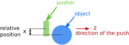
Figure 2: Pushing a circular object with a rectangle pusher.

6.1 Importance of learning accurate models

Our method was designed to be appropriate for use in systems whose dynamics are not well modeled with uni-modal Gaussian noise. The experiments in this section explore the question of whether a uni-modal model could work just as well, using a simple domain with known dynamics $s^{\prime}=s+T(a)\rho$, where the relative position $x=0$ and duration $\Delta t=1$ are fixed, the action is the direction of motion, $a=z\in[0,2\pi)$, $T(a)$ is the rotation matrix for angle, and the noise is

$$\rho\sim 0.6\mathcal{N}(\begin{bmatrix}5.0\\ 5.0\end{bmatrix},\begin{bmatrix}2.0&0.0\\ 0.0&2.0\end{bmatrix})+0.4\mathcal{N}(\begin{bmatrix}5.0\\ -5.0\end{bmatrix},\begin{bmatrix}2.0&0.0\\ 0.0&2.0\end{bmatrix}).$$

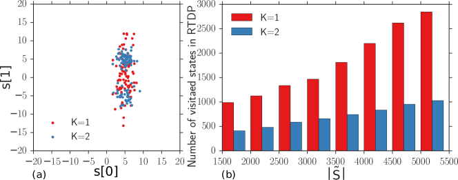
Figure 3: (a) Samples from the single-mode Gaussian transition model ($K=1$) and the two-component Gaussian mixture transition model ($K=2$) in the free space when $a=0$. (b) The number of visited states (y-axis) increases with the number of sampled states $|\tilde{S}|$ (x-axis). Planning with $K=2$ visits fewer states in RTDP than with $K=1$.

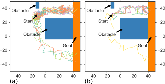
Figure 4: (a) Samples of 10 trajectories with $K=1$. (b) Samples of 10 trajectories with $K=2$. Using the correct number of components for the transition model improves the quality of the trajectories.

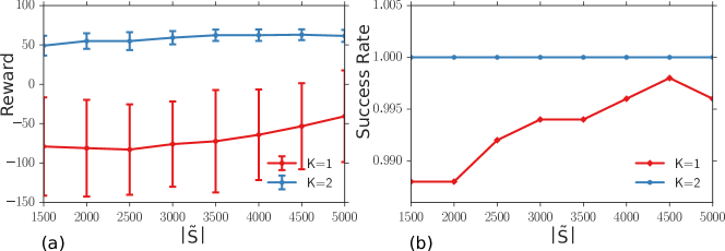
Figure 5: (a): Reward. (b): Success rate. Using two components ($K=2$) performs much better than using one component ($K=1$) in terms of reward and success rate.

We sample $\rho$ from its true distribution and fit a Gaussian ($K=1$) and a mixture of Gaussians ($K=2$). The samples from $K=1$ and $K=2$ are shown in Fig. 3 (a). We plan with both models where each action has an instantaneous reward of $-1$, hitting an obstacle has a reward of $-10$, and the goal region has a reward of $100$. The discount factor $\gamma=0.99$. To show that the results are consistent, we use Algorithm 3 to sample 1500 to 5000 states to construct $\tilde{S}$, and plan with each of them using $100$ uniformly discretized actions within $1000$ iterations of RTDP.

To compute the Monte Carlo reward, we simulated 500 trajectories for each computed policy with the true model dynamics, and for each simulation, at most 500 steps are allowed. We show 10 samples of trajectories for both $K=1$ and $K=2$ with $|\tilde{S}|=5000$, in Fig 4. Planning with the right model $K=2$ tends to find better trajectories, while because $K=1$ puts density on many states that the true model does not reach, the policy of $K=1$ in Fig 4 (a) causes the robot to do extra maneuvers or even choose a longer trajectory to avoid obstacles that it actually has very low probability of hitting. As a result, the reward and success rate for $K=2$ are both higher than $K=1$, as shown in Fig. 5. Furthermore, because the single-mode Gaussian estimates the noise to have a large variance, it causes RTDP to visit many more states than necessary, as shown in Fig. 3 (b).

6.2 Focusing on the good actions and states

In this section we demonstrate the effectiveness of our strategies for limiting the number of states visited and actions modeled. We denote using Bayesian optimization in Lines 11 and 14 in Algorithm 4 as BO and using random selections as Rand.

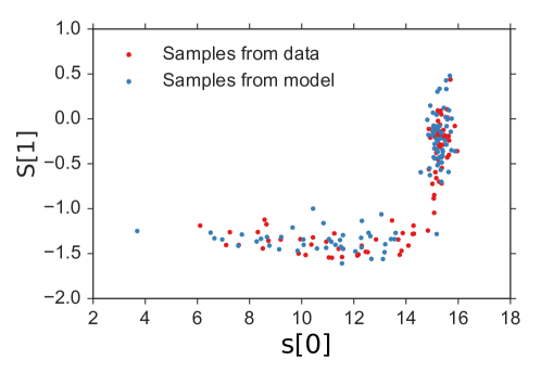
Figure 6: The conditional distribution of $\Delta s$ given $a=(z,x,\Delta t)=(0.0,0.3,2.0)$ is a multi-modal Gaussian.

We first demonstrate why BO is better than random for optimizing $Q_{s}(a)$ with the simple example from Sec. 6.1. We plot the $Q_{s}(a)$ in the first iteration of RTDP where $s=[-4.3,33.8]$, and let random and BO in Algorithm 5 each pick 10 actions to evaluate sequentially as shown in Fig 7 (a). We use the GP implementation and the default Matern52 kernel implemented in the GPy module [11] and optimize its kernel parameters every 5 selections. The first point for both BO and Rand is fixed to be $a=0.0$. We observe that BO is able to focus its action selections in the high-value region, and BO is also able to explore informative actions if it has not found a good value or if it has finished exploiting a good region (see selection 10). Random action selection wastes choices on regions that have already been determined to be bad.

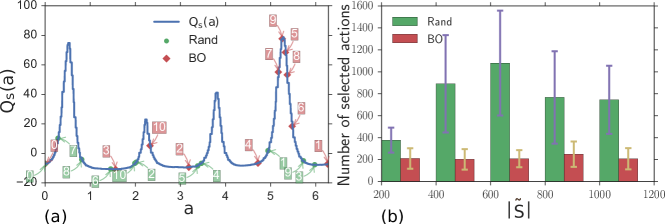
Figure 7: (a) We optimize $Q_{s}(a)$ with BO and Rand by sequentially sampling 10 actions. BO selects actions more strategically than Rand. (b) BO samples fewer actions than Rand in the pushing problem for all settings of $|\tilde{S}|$.

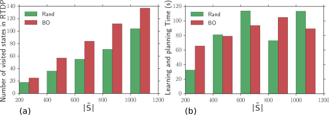
Figure 8: (a) Number of visited states in RTDP. Both of Rand and BO consistently focus on about 10% states for planning. (b) Learning and planning time of BO and Rand.

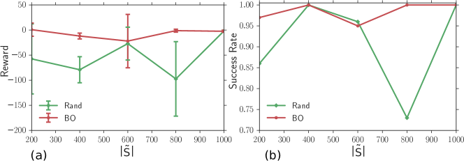
Figure 9: (a) Reward. (b) Success rate. BO achieves better reward and success rate, with many fewer actions and slightly more visited states.

Next we consider a more complicated problem in which the action is the high level control of a pushing problem $a=(z,x,\Delta t)$, $z\in[0,2\pi],x\in[-1.0,1.0],\Delta t\in[0.0,3.0]$ as illustrated in Fig. 2. The instantaneous reward is $-1$ for each free-space motion, $-10$ for hitting an obstacle, and $100$ for reaching the goal; $\gamma=0.99$. We collected $1.2\times 10^{6}$ data points of the form $(a,\Delta s)$ with $x$ and $\Delta t$ as variables in the Box2D simulator [4] where noise comes from variability of the executed action. We make use of the fact that the object is cylindrical (with radius 1.0) to reuse data. An example of the distribution of $\Delta s$ given $a=(0.0,0.3,2.0)$ is shown in Fig. 6.

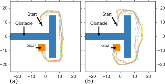
Figure 10: (a) 10 samples of trajectories generated via Rand with 1000 states. (b) 10 samples of trajectories generated via BO with 1000 states.

We compare policies found by Rand and BO with the same set of sampled states ($|\tilde{S}|=200,400,600,800,1000$) within approximately the same amount of total computation time. They are both able to compute the policy in $30\sim 120$ seconds, as shown in Fig. 8 (b). In more realistic domains, it is possible that learning the transition model will take longer and dominate the action-selection computation. We simulate 100 trajectories in the Box2D simulator for each planned policy with a maximum of 200 seconds. We show the result of the reward and success rate in Fig. 9, and the average number of actions selected for visited states in Fig. 7(b). In our simulations, BO consistently performs approximately the same or better than Rand in terms of reward and success rate while BO selects fewer actions than Rand. We show 10 simulated trajectories for Rand and BO with $|\tilde{S}|=1000$ in Fig. 10.

From Fig. 8 (a), it is not hard to see that RTDP successfully controlled the number of visited states to be only a small fraction of the whole sampled set of states. Interestingly, BO was able to visit slightly more states with RTDP and as a result, explored more possible states that it is likely to encounter during the execution of the policy, which may be a factor that contributed to its better performance in terms of reward and success rate in Fig. 9. We did not compare with pure value iteration because the high computational cost of computing models for all the states made it infeasible.

BOIDP is able to compute models for only around 10% of the sampled states and about 200 actions per state. If we consider a naive grid discretization for both action (3 dimension) and state (2 dimension) with 100 cells for each dimension, the number of models we would have to compute is on the order of $10^{10}$, compared to our approach, which requires only $10^{4}$.

7 Conclusion

An important class of robotics problems are intrinsically continuous in both state and action space, and may demonstrate non-Gaussian stochasticity in their dynamics. We have provided a framework to plan and learn effectively for these problems. We achieve efficiency by focusing on relevant subsets of state and action spaces, while retaining guarantees of asymptotic optimality.

References

- [1] Leemon C. Baird, III and A. Harry Klopf. Reinforcement learning with high-dimensional continuous actions. Technical report, Wright Laboratory, Wright Patterson Air Force Base, 1993.
- [2] Andrew G Barto, Steven J Bradtke, and Satinder P Singh. Learning to act using real-time dynamic programming. Artificial Intelligence, 72(1):81–138, 1995.
- [3] Eric Brochu, Vlad M Cora, and Nando De Freitas. A tutorial on Bayesian optimization of expensive cost functions, with application to active user modeling and hierarchical reinforcement learning. Technical Report TR-2009-023, University of British Columbia, 2009.
- [4] Erin Catto. Box2D, a 2D physics engine for games. http://box2d.org, 2011.
- [5] Augustin Louis Cauchy. Cours d’analyse de l’Ecole Royale Polytechnique, volume 1. Imprimerie royale, 1821.
- [6] Marc Deisenroth and Carl E Rasmussen. PILCO: A model-based and data-efficient approach to policy search. In ICML, 2011.
- [7] Marc Peter Deisenroth, Carl Edward Rasmussen, and Jan Peters. Model-based reinforcement learning with continuous states and actions. In ESANN, 2008.
- [8] Marc Peter Deisenroth, Carl Edward Rasmussen, and Jan Peters. Gaussian process dynamic programming. Neurocomputing, 72(7):1508–1524, 2009.
- [9] Marcus Frean and Phillip Boyle. Using Gaussian processes to optimize expensive functions. In Australasian Joint Conference on Artificial Intelligence, 2008.
- [10] Mohammad Ghavamzadeh, Shie Mannor, Joelle Pineau, Aviv Tamar, et al. Bayesian reinforcement learning: A survey. Foundations and Trends in Machine Learning, 8(5–6):359–483, 2015.
- [11] GPy. GPy: A Gaussian process framework in python. http://github.com/SheffieldML/GPy, since 2012.
- [12] V. Gullapalli, J. A. Franklin, and H. Benbrahim. Acquiring robot skills via reinforcement learning. IEEE Control Systems, 14(1):13–24, 1994.
- [13] Vu Anh Huynh, Sertac Karaman, and Emilio Frazzoli. An incremental sampling-based algorithm for stochastic optimal control. IJRR, 35(4):305–333, 2016.
- [14] Hunor S Jakab and Lehel Csató. Reinforcement learning with guided policy search using Gaussian processes. In IJCNN, 2012.
- [15] Marek Kopicki. Prediction learning in robotic manipulation. PhD thesis, University of Birmingham, 2010.
- [16] Marek Kopicki, Jeremy Wyatt, and Rustam Stolkin. Prediction learning in robotic pushing manipulation. In ICAR, 2009.
- [17] Marek Kopicki, Sebastian Zurek, Rustam Stolkin, Thomas Mörwald, and Jeremy Wyatt. Learning to predict how rigid objects behave under simple manipulation. In ICRA, 2011.
- [18] Steven M LaValle. Rapidly-exploring random trees: A new tool for path planning. Technical Report TR 98-11, Computer Science Dept., Iowa State University, 1998.
- [19] Christopher R Mansley, Ari Weinstein, and Michael L Littman. Sample-based planning for continuous action markov decision processes. In ICAPS, 2011.
- [20] Ankur Moitra and Gregory Valiant. Settling the polynomial learnability of mixtures of gaussians. In FOCS, 2010.
- [21] Teodor Mihai Moldovan, Sergey Levine, Michael I Jordan, and Pieter Abbeel. Optimism-driven exploration for nonlinear systems. In ICRA, 2015.
- [22] Duy Nguyen-Tuong and Jan Peters. Model learning for robot control: A survey. Cognitive processing, 12(4):319–340, 2011.
- [23] Barry D. Nichols. Continuous action-space reinforcement learning methods applied to the minimum-time swing-up of the acrobot. In ICSMC, 2015.
- [24] D. V. Prokhorov and D. C. Wunsch. Adaptive critic designs. IEEE Trans. Neural Networks, 8(5):997–1007, 1997.
- [25] Carl Edward Rasmussen and Christopher KI Williams. Gaussian processes for machine learning. The MIT Press, 2006.
- [26] Axel Rottmann and Wolfram Burgard. Adaptive autonomous control using online value iteration with Gaussian processes. In ICRA, 2009.
- [27] Niranjan Srinivas, Andreas Krause, Sham M Kakade, and Matthias Seeger. Gaussian process optimization in the bandit setting: No regret and experimental design. In ICML, 2010.
- [28] Richard S Sutton and Andrew G Barto. Reinforcement learning: An introduction, volume 1. MIT press Cambridge, 1998.
- [29] Michalis K Titsias and Miguel Lázaro-Gredilla. Variational heteroscedastic Gaussian process regression. In ICML, 2011.
- [30] Matteo Turchetta, Felix Berkenkamp, and Andreas Krause. Safe exploration in finite Markov decision processes with Gaussian processes. In NIPS, 2016.
- [31] Hado van Hasselt and Marco A. Wiering. Reinforcement learning in continuous action spaces. In ICAR, 2007.
- [32] Zi Wang, Bolei Zhou, and Stefanie Jegelka. Optimization as estimation with Gaussian processes in bandit settings. In AISTATS, 2016.
- [33] Ari Weinstein and Michael L Littman. Bandit-based planning and learning in continuous-action Markov decision processes. In ICAPS, 2012.
- [34] Dominik Wied and Rafael Weißbach. Consistency of the kernel density estimator: a survey. Statistical Papers, 53(1):1–21, 2012.
- [35] Timothy Yee, Viliam Lisy, and Michael Bowling. Monte carlo tree search in continuous action spaces with execution uncertainty. In IJCAI, 2016.
- [36] Kuan-Ting Yu, Maria Bauza, Nima Fazeli, and Alberto Rodriguez. More than a million ways to be pushed: A high-fidelity experimental data set of planar pushing. In IROS, 2016.
- [37] Chao Yuan and Claus Neubauer. Variational mixture of Gaussian process experts. In NIPS, 2009.