Graphene pn junction in a quantizing magnetic field: Conductance at intermediate disorder strength

Abstract

In a graphene pn junction at high magnetic field, unidirectional “snake states” are formed at the pn interface. In a clean pn junction, each snake state exists in one of the valleys of the graphene band structure, and the conductance of the junction as a whole is determined by microscopic details of the coupling between the snake states at the pn interface and quantum Hall edge states at the sample boundaries [Tworzydlo et al., Phys. Rev. B 76, 035411 (2007)]. Disorder mixes and couples the snake states. We here report a calculation of the full conductance distribution in the crossover between the clean limit and the strong disorder limit, in which the conductance distribution is given by random matrix theory [Abanin and Levitov, Science 317, 641 (2007)]. Our calculation involves an exact solution of the relevant scaling equation for the scattering matrix, and the results are formulated in terms of parameters describing the microscopic disorder potential in bulk graphene.

I Introduction

Many of the unique electronic properties of graphene, a single layer of carbon atoms as they occur in graphite, can be traced back to its pseudorelativistic band structure, in which quasiparticles behave as massless relativistic Dirac particles, be it with the Fermi velocity $v_{\rm F}$ instead of the speed of light $c$. Castro Neto et al. (2009); Das Sarma et al. (2011); Peres (2010) Examples of such “relativistic” effects in graphene are Klein tunneling through potential barriers, Klein (1929); Cheianov and Falko (2006); Katsnelson et al. (2006); Beenakker (2008) the Zitterbewegung in confining potentials,Katsnelson et al. (2006) the anomalous integer quantum Hall effect, Gusynin and Sharapov (2005); Novoselov et al. (2005); Zhang et al. (2005); Novoselov et al. (2007) or the breakdown of Landau quantization in crossed electric and magnetic fields. Lukose et al. (2007); Peres and Castro (2007)

The integer quantum Hall effect in graphene is called “anomalous” because the number of chiral edge states at the boundary of a graphene flake in a large perpendicular magnetic field is a multiple of four plus two, whereas the Dirac bands are fourfold degenerate because of the combined spin and valley degeneracies. The presence of a “half” edge mode per valley degree of freedom has a direct explanation once it is taken into account that the valley degeneracy is necessarily lifted at a graphene flake’s outer boundaries. Brey and Fertig (2006) Chiral states need not only occur at a flake’s outer boundaries, but they may also occur in the sample’s interior, separating regions with different electron density. At such an interface valley degeneracy is usually preserved, and the number of chiral interface states is always a multiple of four.

A particularly interesting realization of such an interface occurs at a pn junction in a perpendicular magnetic field, separating hole-doped (p-type) and electron-doped (n-type) graphene regions. Williams et al. (2007); Lohmann et al. (2009); Ki and Lee (2009) The edge states at the pn interface are referred to as “snake states” because, at least in a semiclassical picture, such states propagate alternatingly at the $p$ and $n$ sides of the junction, Williams and Marcus (2011); Rickhaus et al. (2015) similar to the behavior of the states that propagate along zero-field contours in the quantum Hall insulators in an inhomogeneous magnetic field. Müller (1992); Ye et al. (1995); Reijniers and Peeters (2000); Ghosh et al. (2008) A graphene pn junction also has edge states at the sample boundaries, which move in opposite directions in the p and n-type regions, see Fig. 1, and feed into/flow out of the snake states at the pn interface.

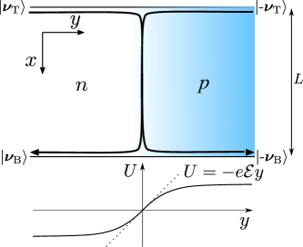
Figure 1: (Color online) Schematic experimental setup of a graphene pn-junction in a quantizing magnetic field, such that the n region has filling fraction $2$ (left) and the p region has filling fraction $-2$ (right). At the pn interface there is a fourfold degenerate chiral interface state; there are twofold degenerate chiral edge states at the sample’s top and bottom edge.

The minimal number of chiral edge and interface states is realized for a pn junction with filling fractions $2$ and $-2$. In this case there are two edge modes, one for each spin direction, and four chiral interface modes. The two-terminal conductance $G$ of such a pn junction is determined by the probability $T$ that an electron that enters the common edge at the pn interface from the source reservoir is transmitted to the drain reservoir,

$$G=\frac{2e^{2}}{h}T\,.$$ (1)

In the limit of a strongly disordered pn interface, Abanin and Levitov predicted that the probability $T$ itself is subject to mesoscopic fluctuations, Abanin and Levitov (2007) with average $\langle T\rangle=1/2$ and variance $\mbox{var}\,T=1/12$. In the opposite limit of an ideal graphene sheet, Tworzydlo et al. foundTworzydło et al. (2007)

$$T=\frac{1}{2}(1-\bm{\nu}_{\rm T}\cdot\bm{\nu}_{\rm B})\,,$$ (2)

where the “isospin” vectors $\bm{\nu}_{\rm T}$ and $\bm{\nu}_{\rm B}$ describe the precise way in which the valley degeneracy is broken at the sample boundaries, see Fig. 1. Subsequent theoretical work involved a semiclassical analysis, Carmier et al. (2010, 2011) numerical simulations of the effect of disorder Li and Shen (2008); Long et al. (2008) and a phenomenological inclusion of dephasing. Chen et al. (2011) Several experimental groups have performed measurements of the two-terminal conductance of graphene pn junctions in a large perpendicular magnetic field. Williams et al. (2007); Lohmann et al. (2009); Ki and Lee (2009); Ki et al. (2010); Woszczyna et al. (2011); Williams and Marcus (2011); Schmidt et al. (2013); Matsuo et al. (2015a); Klimov et al. (2015) The measured conductance follows the ensemble average of the strongly disordered limit of Ref. Abanin and Levitov, 2007, although the experimentally observed mesoscopic fluctuations remain significantly below the theoretical prediction. Measurements of the shot noise power find a value that approaches the theoretical prediction for the shortest interface lengths. Matsuo et al. (2015b); Kumada et al. (2015)

In this article we present a theory of the transmission probability $T$ for a graphene pn junction with generic disorder. We focus on the case of filling fractions $(\nu_{n},\nu_{p})=(2,-2)$, for which we give an exact solution for the distribution of the transmission probability $T$, thus bridging the gap between the clean limit of Ref. Tworzydło et al., 2007 and the strong-disorder limit of Ref. Abanin and Levitov, 2007. Knowledge of the distribution of $T$ allows us to calculate the average conductance $G$, its variance, and the Fano factor $F$ throughout the weak-to-strong disorder crossover. There are two reasons why we focus on the case $(\nu_{n},\nu_{p})=(2,-2)$ for our exact solution. First, as we show below, two length scales suffice to describe the effect of generic disorder on the edge states, which is an essential simplification that makes our exact solution possible. Second, quantum interference effects are strongest in this case, so that the need for an exact treatment is maximal. Our results for the case $(\nu_{n},\nu_{p})=(2,-2)$ also apply to higher filling fractions, if the mixing of interface states occurs for the lowest Landau lavel only. Klimov et al. (2015)

The problem we consider here is related to two different problems that have been studied in the literature, and we wish to comment on both. First, the study is reminiscent of that of transport in coupled one-dimensional channels with disorder, a problem that was solved exactly already in the 1950s, in the context of wave propagation through random media. Gertsenshtein and Vasil’ev (1959a, b) A crucial difference between the two problems is, however, that all one-dimensional modes at the pn interface propagate in the same direction, whereas a normal metal wire has equal numbers of modes propagating in both directions. This difference leads to a rather different phenomenology: Whereas transmission is exponentially suppressed for sufficiently strong disorder or long length in the standard case, Mott and Twose (1961) for the chiral interface states at a pn junction the probability that electrons are transmitted along the interface is always one. The question is whether they are fed into an edge state that transfers them back to the source reservoir, or into the edge that leads to the drain.

The second related problem is that of the parametric dependence of transport properties in mesoscopic samples. Traditionally (and correctly), it is the Hamiltonian that is taken to depend on an external parameter, such as the magnetic field or a gate voltage, either by modeling the perturbation directly, or in a stochastic manner through a “Brownian motion” process. In a second step the transport properties are then calculated from the Hamiltonian. There have been theoretical attempts to make a theory directly for the parameter dependence of the scattering matrix, e.g., through a modification of Dyson’s Brownian motion model, but such an approach could not be made to agree with the Hamiltonian-based approach if the dimension of the scattering matrix is small.Macêdo (1994, 1996); Frahm and Pichard (1995); Rau (1995) Interestingly, we find that the dependence of the scattering matrix of the interface states on the interface length is precisely described by the Dyson Brownian motion model. To our knowledge, this constitutes the first application of this model to a quantum transport problem.

The article is organized as follows. In Sec. II we outline the microscopic model of a disordered graphene pn-junction and derive an effective one-dimensional Hamiltonian for the chiral interface states in the presence of generic disorder. In Sec. III, we then derive and solve the Fokker-Planck equation describing the diffusive transport through the pn-junction. Using the probability distribution of the scattering matrix, we obtain an expression for the conductance and its variance, being valid for an arbitrary disorder strengths. We conclude in Sec. IV

II Microscopic Model

We choose coordinates such that the pn interface is along the $x$ direction, see Fig. 1. At low energies conduction electrons in the graphene pn junction are described by a $4\times 4$ matrix Hamiltonian,

$$\hat{H}=\hat{H}_{0}+\hat{V}({\bf{r}})\,,$$ (3)

in which $\hat{V}({\bf{r}})$ in Eq. (3) is a matrix-valued potential representing the disorder and

$$\hat{H}_{0}=\tau_{0}\otimes\sigma_{0}U(y)+v_{\rm F}\tau_{3}\otimes(\sigma_{1}\pi_{1}({\bf{r}})+\sigma_{2}\pi_{2}({\bf{r}}))\,.$$ (4)

Here the $\tau_{\mu}$ and $\sigma_{\mu}$ are Pauli matrices acting in valley and sublattice space, respectively, $U(y)$ is a gate potential that defines the p and n-type regions, and $\pi_{1}({\bf{r}})$ and $\pi_{2}({\bf{r}})$ are the in-plane components of the kinematic momentum,

$$\pi_{1}({\bf{r}}) =-i\hbar\partial_{x}-eA_{x}({\bf{r}})\,,$$

$$\pi_{2}({\bf{r}}) =-i\hbar\partial_{y}-eA_{y}({\bf{r}})\,.$$ (5)

Since spin-orbit coupling is weak in graphene, the spin degree of freedom will be suppressed throughout.

For the vector potential we take the asymmetric gauge

$$A_{1}({\bf{r}})=-{\cal B}y\,,\ \ A_{2}({\bf{r}})=0\,,$$ (6)

with ${\cal B}>0$ the perpendicular magnetic field. The magnetic field defines the length scale $\ell=(e{\cal B})^{-1/2}$. The gate potential $U(y)$ is negative for $y<0$, zero for $y=0$, and positive for $y>0$, so that the pn interface is at $y=0$ precisely, see Fig. 1. In the limit of a large magnetic field, it is sufficient to expand $U(y)$ to linear order in $y$ for $|y|\lesssim\ell$, and we set

$$U(y)=-e{\cal E}y\,.$$ (7)

In order to describe graphene with generic disorder we expand the matrix-valued disorder potential $\hat{V}({\bf{r}})$ asAleiner and Efetov (2006); Altland (2006); Ostrovsky et al. (2006)

$$\hat{V}(\bm{r})=\sum_{\mu,\nu=0}^{3}V_{\mu\nu}(\bm{r})\tau_{\mu}\otimes\sigma_{\nu}\,,$$ (8)

with real amplitudes $V_{\mu\nu}(\bm{r})$. We assume these amplitudes to be Gaussian correlated with vanishing mean and with correlation function

$$\langle V_{\mu\nu}(\bm{r})V_{\mu^{\prime}\nu^{\prime}}(\bm{r}^{\prime})\rangle =\Gamma_{\mu\nu}\delta_{\mu\mu^{\prime}}\delta_{\nu\nu^{\prime}}\delta(\bm{r}-\bm{r}^{\prime})\,,$$ (9)

where the absence of correlations between different amplitudes is a consequence of translation and rotation symmetry on the average.Ostrovsky et al. (2006) The same symmetry considerations reduce the number of independent correlators to nine,

$$\Gamma_{\mu\nu}=\begin{pmatrix}\alpha_{0}&\gamma_{\perp}&\gamma_{\perp}&\alpha_{z}\\ \beta_{z}&\beta_{\perp}&\beta_{\perp}&\beta_{0}\\ \beta_{z}&\beta_{\perp}&\beta_{\perp}&\beta_{0}\\ \gamma_{0}&\alpha_{\perp}&\alpha_{\perp}&\gamma_{z}\end{pmatrix},$$ (10)

such that the five parameters $\alpha_{0}$, $\beta_{\perp}$, $\beta_{z}$, $\gamma_{\perp}$, and $\gamma_{z}$ represent disorder contributions respecting time-reversal-symmetry,Aleiner and Efetov (2006); Altland (2006) whereas the remaining four parameters $\alpha_{\perp}$, $\alpha_{z}$, $\beta_{0}$, and $\gamma_{0}$ represent time-reversal-symmetry-breaking disorder. The coefficient $\alpha_{0}$ represents potential disorder that is smooth on the scale of the lattice spacing; the coefficients $\beta_{\perp}$ and $\gamma_{z}$ appear if the potential disorder is short range, so that it couples to the valley and sublattice degrees of freedom. The other coefficients are associated with a (random) magnetic field, strain, or lattice defects, see Ref. Ostrovsky et al., 2006. Since time-reversal symmetry is broken by the large magnetic field ${\cal B}$, we will consider all nine contributions.

With a large magnetic field ${\cal B}$ the low-energy degrees of freedom of the Hamiltonian (3) are the two chiral one-dimensional modes at the pn interface (per spin direction). They are described by an effective Hamiltonian

$$H_{\rm s}=-i\hbar v_{\rm s}\tau_{0}\partial_{x}+\sum_{\mu=0}^{3}V_{{\rm s},\mu}(x)\tau_{\mu}\,,$$ (11)

where $v_{\rm s}$ is the velocity of the interface modes and the $V_{{\rm s},\mu}(x)$ are effective disorder potentials representing the effect of the bulk disorder potential $\hat{V}({\bf{r}})$ on the interface states. In the limit of a large magnetic field, we can find exact expressions for $v_{\rm s}$ and for the correlation functions of the disorder potential $V_{\rm s}$ in terms of the parameters of the underlying two-dimensional Hamiltonian (3). The linear approximation (7) for the gate potential $U$ allows us to make use of an exact solution for the eigenstates of the Hamiltonian $H_{0}$ of Eq. (4).Peres and Castro (2007); Lukose et al. (2007) [See Ref. Liu et al., 2015 for an approximate solution that does not make use of the linear approximation (7).] Furthermore, for large magnetic fields the Landau level separation is large enough that only the zeroth Landau level needs to be considered. With the help of the exact solution for the zeroth Landau level we then find that the velocity of the interface modes is

$$v_{\rm s}={\cal E}/{\cal B}\,,$$ (12)

whereas the disorder potentials $V_{{\rm s},\mu}(x)$ have zero mean and correlation functions

$$\langle V_{{\rm s},\mu}(x)V_{{\rm s},\nu}(x^{\prime})\rangle =K_{\mu}\delta_{\mu\nu}\delta(x-x^{\prime})\,,$$ (13)

with, to leading order in $v_{\rm s}/v_{\rm F}\ll 1$,

$$K_{0}(\alpha_{0},\alpha_{z},\alpha_{\perp}) =\frac{1}{\sqrt{2\pi\ell^{2}}}\left(\alpha_{0}+\alpha_{z}\right)\,,$$ (14a)

$$K_{1,2}(\beta_{0},\beta_{z},\beta_{\perp}) =\frac{1}{\sqrt{2\pi\ell^{2}}}\left(\beta_{0}+\beta_{z}\right)\,,$$ (14b)

$$K_{3}(\gamma_{0},\gamma_{z},\gamma_{\perp}) =\frac{1}{\sqrt{2\pi\ell^{2}}}\left(\gamma_{0}+\gamma_{z}\right)\,.$$ (14c)

The microscopic amplitudes $\alpha_{\perp},\beta_{\perp},\gamma_{\perp}$ contribute only at higher orders in $v_{\rm s}/v_{\rm F}$. We refer to App. A for details of the calculation.

III Scaling approach for the scattering matrix

Disorder mixes the chiral interface modes. The effect of this disorder-induced mode mixing is described by a $2\times 2$ scattering matrix $\hat{S}$. In the absence of disorder one has $\hat{S}=e^{ikL}\openone$. With disorder $\hat{S}$ acquires a nontrivial probability distribution $P(\hat{S})$, which we now calculate.

We parametrize the scattering matrix using four “angles”,

$$\hat{S}=e^{i\psi\tau_{0}}e^{i\tau_{3}\varphi/2}e^{i\tau_{2}\theta/2}e^{i\tau_{3}\zeta/2}\,,$$ (15)

where $\theta\in[0,\pi]$. We will first derive a differential equation that describes the change of the joint distribution $P(\varphi,\theta,\zeta,\psi;L)$ upon changing the length $L$ of the interface region, see Fig. 1. To this end, we consider the scattering matrix $\hat{S}_{\delta L}$ for an interface segment of length $\delta L$ much smaller than the mean free path for disorder scattering. We parametrize $\hat{S}_{\delta L}$ as

$$\hat{S}_{\delta L}=e^{ik\delta L}e^{i\hat{A}}\,,\ \ \hat{A}=\sum_{\mu=0}^{3}r_{\mu}\tau_{\mu}\,.$$ (16)

From the effective Hamiltonian (11) we find that the coefficients $r_{\mu}$ are statistically independent, with disorder averages $\langle r_{\mu}\rangle=0$, $\mu=0,1,2,3$, and with variances

$$\langle r_{\mu}^{2}\rangle=\frac{K_{\mu}}{\hbar^{2}v_{\rm s}^{2}}\delta L\,,$$ (17)

with the coefficients $K_{\mu}$ given in Eq. (14). To simplify the expressions in the remainder of this Section, we replace the notation with the coefficients $K_{\mu}$ in favor of the inter-valley scattering length

$$l_{\rm i}=\frac{\hbar^{2}v_{\rm s}^{2}}{4K_{1}}\,,$$ (18)

the (antisymmetric) intra-valley scattering length

$$l_{\rm a}=\frac{\hbar^{2}v_{\rm s}^{2}}{4K_{3}}\,,$$ (19)

and the dimensionless coefficients

$$\alpha=K_{0}/4K_{1}\,,\ \ \gamma=K_{3}/K_{1}=l_{\rm i}/l_{\rm a}\,,$$ (20)

which relate inter- and intra-valley scattering rates. In the case of pure potential disorder, only the disorder coefficients $\alpha_{0}$, $\beta_{\perp}$, and $\gamma_{z}$ are nonzero, so that the constants $\alpha$, $\gamma\sim(v_{\rm F}/v_{\rm s})^{2}\gg 1$. For generic disorder that scatters between the two sublattices of the hexagonal graphene lattice, one expects that $\alpha$, $\gamma\sim 1$. The parameters $\alpha$ and $\gamma$ determine symmetric and antisymmetric intra-valley scattering lengths, respectively. Since intra-valley scattering that is equal for the two valleys corresponds to multiplication of $\hat{S}$ with an overall phase factor, the coefficient $\alpha$ will not appear in the expressions for the conductance distribution below. Antisymmetric intravalley scattering, however, does affect the transmission probability $T$ of the pn junction.

Since the interface modes are unidirectional, the composition rule for scattering matrices is matrix multiplication. In particular, we obtain the scattering matrix $\hat{S}(L+\delta L)$ of an interface segment of length $L+\delta L$ as

$$\hat{S}(L+\delta L)=\hat{S}(L)\hat{S}_{\delta L}\,.$$ (21)

This composition rule and the known statistical distribution of the scattering matrices $\hat{S}_{\delta L}$ define a “Brownian motion” problem for the scattering matrix $\hat{S}(L)$. An isotropic version of the Brownian motion problem, with $\alpha=\gamma=1$, was studied previously in the context of quantum transport through chaotic quantum dots.Macêdo (1994, 1996); Frahm and Pichard (1995); Rau (1995) Using standard methods (see App. B for details), we can derive a Fokker-Planck equation for the joint probability distribution $P(\varphi,\theta,\zeta,\psi;L)$ of the coefficients parametrizing the scattering matrix $\hat{S}$,

$$l_{\rm i}\frac{\partial P}{\partial L}= -kl_{\rm i}\frac{\partial P}{\partial\psi}+\frac{1}{2}\alpha\frac{\partial^{2}P}{\partial\psi^{2}}+\frac{1}{2}\left(\gamma+\cot^{2}\theta\right)\frac{\partial^{2}P}{\partial\zeta^{2}}$$

$$+\frac{1}{2}\frac{\partial^{2}P}{\partial\theta^{2}}-\frac{1}{2}\cot\theta\frac{\partial P}{\partial\theta}+\frac{1}{2}\csc^{2}\theta\frac{\partial^{2}P}{\partial\varphi^{2}}$$

$$-\cot\theta\csc\theta\frac{\partial^{2}P}{\partial\varphi\partial\zeta}+\frac{1}{2}\csc^{2}\theta P\,.$$ (22)

The Fokker-Planck equation Eq. (22) for the $L$ dependence of the scattering matrix of two co-propagating modes can be solved exactly by adapting Ancliff’s method to solve the corresponding problem for a pair of counterpropagating modes.Ancliff (2016) After separating variables

$$P(L,\varphi,\theta,\zeta,\psi)=e^{-\lambda L/l_{\rm i}}P(\varphi,\theta,\zeta,\psi)\,,$$ (23)

Eq. (22) can be cast in the form of an eigenvalue problem, which, following Ref. Ancliff, 2016, can be solved exactly by noticing that its right hand-side can be expressed through the operator $\hat{A}$ defined in Eq. (16), seen as a differential operator acting in the Hilbert space of functions $f(\hat{S})$,

$$\langle\hat{A}^{2}\rangle=-\left(\hat{L}_{x}^{2}+\hat{L}_{y}^{2}+\hat{L}_{z}^{2}+(\gamma-1)\hat{L}_{z}^{2}+\alpha\hat{L}_{0}^{2}\right)\,,$$ (24)

in which the operators $\hat{L}_{\mu}$ are the generators of the Lie algebra $\mathfrak{u}(2)$. The Lie algebra $\mathfrak{u}(2)$ has two Casimir operators, $\hat{L}_{0}$ and $\hat{\bm{L}}^{2}=\hat{L}_{x}^{2}+\hat{L}_{y}^{2}+\hat{L}_{z}^{2}$, that act as scalars $K$ and $l(l+1)$ ($l$ being integer or half-integer, $K$ being a real number), respectively, within each irreducible representation of $U(2)$. Thus we can conclude immediately that the eigenvalues associated to the eigenvalue problem obtained from Eq. (22) are of the form

$$-\lambda_{Klm} =l(l+1)+(\gamma-1)m^{2}+\alpha K^{2}+2ikl_{\rm i}K,$$ (25)

where $m=-l,-l+1,\ldots,l$ and we included the drift term for $\psi$ being proportional to $kl_{\rm i}$, which is not contained in Eq. (24). The eigenfunctions can be expressed Landau and Lifshitz (1991) in terms of Jacobi polynomials $P^{(a,b)}_{n}$ ($|m|\leq l$)

$$P_{Klmn} =\sqrt{\frac{(l+m)!(l-m)!}{(l+n)!(l-n)!}}e^{iK\psi}e^{im\varphi+in\zeta}\sin\theta$$ (26)

$$\times\sin^{m-n}(\theta/2)\cos^{m+n}(\theta/2)P_{j-m}^{(m-n,m+n)}(\cos\theta)\,.$$

For $m=n=0$ these eigenfunctions match the ones previously obtained by Frahm and Pichard for the isotropic scattering matrix Brownian motion problem. Frahm and Pichard (1995) It can be readily checked that the above functions for arbitrary $K$, $l$, $m$, and $n$ are simultaneously eigenfunctions of $\hat{\bm{L}}^{2}$, $\hat{L}_{z}$ and $\hat{L}_{0}$ and that they satisfy the eigenvalue equation derived from Eq. (22) with eigenvalues given by Eq. (25).

As the initial condition at $L=0$ we take $\hat{S}(0)=\openone$, which corresponds to

$$P(\varphi,\theta,\zeta,\psi;0)=\delta(\varphi+\zeta)\delta(\theta)\delta(\psi)\,.$$ (27)

With this initial condition the solution for the probability distribution is

$$P(\varphi,\theta,\zeta,\psi;L)= \sqrt{\frac{l_{\rm i}}{2\pi\alpha L}}e^{-\frac{l_{\rm i}(\psi-kL)^{2}}{2\alpha L}}\sum_{l}\frac{2l+1}{8\pi^{2}}\sin\theta$$

$$\times\sum_{m=-l}^{l}e^{-[l(l+1)+(\gamma-1)m^{2}]L/l_{\rm i}+im(\varphi+\zeta)}$$

$$\times\cos^{2m}(\theta/2)P_{l-m}^{(0,2m)}(\cos\theta)\,.$$ (28)

The scattering matrix $\hat{S}$ is related to the transmission probability $T$ of a graphene pn junction through the relation Tworzydło et al. (2007)

$$T =|\langle\bm{\nu}_{\rm T}|\hat{t}_{\rm T}\hat{S}\hat{t}_{\rm B}|-\bm{\nu}_{\rm B}\rangle|^{2}\,,$$ (29)

in which $\hat{t}_{\rm T}$ ($\hat{t}_{\rm B}$) is the scattering matrix describing how the edge modes at the top (bottom) edges of the pn junction feed into/originate from the interface modes and $|\pm\bm{\nu}_{T}\rangle$ ($|\pm\bm{\nu}_{B}\rangle$) are valley isospin Bloch vectors for the top (bottom) edges of the n ($+$) and p-doped ($-$) regions, see Fig. 1. The isospin vectors $|\bm{\nu}_{X}\rangle$ are superpositions of the vectors $|1\rangle$ and $|-1\rangle$ representing the two valleys,

$$|\bm{\nu}_{X}\rangle= \cos\frac{\theta_{X}}{2}|1\rangle+e^{i\phi_{X}}\sin\frac{\theta_{X}}{2}|-1\rangle\,,$$

$$|-\bm{\nu}_{X}\rangle= \sin\frac{\theta_{X}}{2}|1\rangle-e^{i\phi_{X}}\cos\frac{\theta_{X}}{2}|-1\rangle\,,$$ (30)

with polar angles $\theta_{X}$ and $\phi_{X}$, $X={\rm T}$, ${\rm B}$. The scattering matrices $\hat{t}_{\rm T}$ and $\hat{t}_{\rm B}$ express isospin conservation at the point where the valley-non-degenerate edge states merge into/evolve out of the valley degenerate interface state, Tworzydło et al. (2007)

$$\hat{t}_{X}=e^{i\tilde{\varphi}_{X}}|\bm{\nu}_{X}\rangle\langle\bm{\nu}_{X}|+e^{i\tilde{\varphi}_{X}^{\prime}}|-\bm{\nu}_{X}\rangle\langle-\bm{\nu}_{X}|\,,$$ (31)

with $\tilde{\varphi}_{X}$ and $\tilde{\varphi}_{X}^{\prime}$ arbitrary phases that do not need to be specified. Combination of Eqs. (29) and (31) givesTworzydło et al. (2007)

$$T =|\langle\bm{\nu}_{\rm T}|\hat{S}|-\bm{\nu}_{\rm B}\rangle|^{2}\,.$$ (32)

Using Eq. (15) as well as the fact that the phase difference $\varphi-\zeta$ is uniformly distributed for all $L$, we find that the disorder average $\langle T\rangle$ is given by

$$\langle T\rangle= \frac{1}{2}\Big{[}1-\cos\theta_{\rm T}\cos\theta_{\rm B}\langle\cos\theta\rangle$$ (33)

$$-\sin\theta_{\rm T}\sin\theta_{\rm B}\langle\cos\theta\cos(\varphi+\phi_{\rm T})\cos(\zeta-\phi_{\rm B})\rangle$$

$$+\sin\theta_{\rm T}\sin\theta_{\rm B}\langle\sin(\varphi+\phi_{\rm T})\sin(\zeta-\phi_{\rm B})\rangle\Big{]}\,.$$

Using the probability distribution (28) one then finds the remarkably simple result

$$\langle T\rangle= \frac{1}{2}\Big{[}1-e^{-2L/l_{\rm i}}\cos\theta_{\rm T}\cos\theta_{\rm B}$$

$$-e^{-L/l_{\rm i}-L/l_{\rm a}}\sin\theta_{\rm T}\sin\theta_{\rm B}\cos(\phi_{\rm T}-\phi_{\rm B})\Big{]}\,.$$ (34)

Similarly we obtain the variance of the transmission probability

$$\text{var}\,T =\frac{1}{12}-\frac{1}{4}e^{-4L/l_{\rm i}}\cos^{2}\theta_{\rm T}\cos^{2}\theta_{\rm B}$$ (35)

$$+\frac{1}{24}e^{-6L/l_{\rm i}}(3\cos^{2}\theta_{\rm T}-1)(3\cos^{2}\theta_{\rm B}-1)$$

$$-\frac{1}{4}e^{-2L/l_{\rm i}-2L/l_{\rm a}}\cos^{2}(\phi_{\rm T}-\phi_{\rm B})\sin^{2}\theta_{\rm T}\sin^{2}\theta_{\rm B}$$

$$+\frac{1}{8}e^{-2L/l_{\rm i}-4L/l_{\rm a}}\cos 2(\phi_{\rm T}-\phi_{\rm B})\sin^{2}\theta_{\rm T}\sin^{2}\theta_{\rm B}$$

$$+\frac{1}{8}e^{-5L/l_{\rm i}-L/l_{\rm a}}\cos(\phi_{\rm T}-\phi_{\rm B})\sin(2\theta_{\rm T})\sin(2\theta_{\rm B})$$

$$-\frac{1}{8}e^{-3L/l_{\rm i}-L/l_{\rm a}}\cos(\phi_{\rm T}-\phi_{\rm B})\sin(2\theta_{\rm T})\sin(2\theta_{\rm B})\,.$$

In the isotropic case, $\gamma=l_{\rm i}/l_{\rm a}=1$, these expressions can be further simplified, such that $\langle T\rangle$ and $\mbox{var}\,T$ depend on the scalar product $\bm{\nu}_{\rm T}\cdot\bm{\nu}_{\rm B}$ of the isospin vectors only,

$$\langle T\rangle= \frac{1}{2}\left(1-e^{-2L/l_{\rm i}}\bm{\nu}_{\rm T}\cdot\bm{\nu}_{\rm B}\right)\,,$$ (36)

$$\text{var}\,T= \frac{1}{12}-\frac{1}{4}e^{-4L/l_{\rm i}}(\bm{\nu}_{\rm T}\cdot\bm{\nu}_{\rm B})^{2}$$

$$+\frac{1}{4}e^{-6L/l_{\rm i}}\left((\bm{\nu}_{\rm T}\cdot\bm{\nu}_{\rm B})^{2}-\frac{1}{3}\right)\,,$$ (37)

In the limiting cases $L\ll l_{\rm i}$, $l_{\rm a}$ and $L\gg l_{\rm i}$, $l_{\rm a}$ Eqs. (34) and (35) [or (37)] agree with the known results for the clean and dirty limits, respectively, see Refs. Abanin and Levitov, 2007 and Tworzydło et al., 2007.

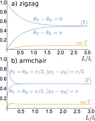
Figure 2: (Color online) Mean $\langle T\rangle$ and variance $\mbox{var}\,T$ of the transmission $T$, as a function of the interface length $L$, for $\gamma=l_{\rm i}/l_{\rm a}=10$. Panel a shows results for zigzag termination of the hexagonal lattice at the top and bottom edges; panel b is for armchair termination. The top curve for $\mbox{var}\,T$ in panel b is for $|\phi_{\rm T}-\phi_{\rm B}|=\pi/3$; the bottom variance curve is for $|\phi_{\rm T}-\phi_{\rm B}|=\pi$.

Figure 2 shows the ensemble average $\langle T\rangle$ and the variance $\mbox{var}\,T$ for representative lattice terminations at the top and bottom edges of the pn junction. For zigzag termination, one has $|\bm{\nu}_{X}\cdot\bm{e}_{z}|=1$, so that the difference $\theta_{\rm T}-\theta_{\rm B}=0$ or $\pi$. Which of these two values is taken depends on the parity of the number of hexagons along the interface length $L$.Tworzydło et al. (2007) For armchair termination one has $\bm{\nu}_{X}\cdot\bm{e}_{z}=0$, so that $\theta_{\rm T}=\theta_{\rm B}=0$. The difference $\phi_{\rm T}-\phi_{\rm B}$ of the azimuthal angles can take the three values $\pi$ and $\pm\pi/3$, depending on the number of hexagons along the interface length $L$ modulo $3$. For the zigzag nanoribbon termination, the crossover between the clean and strong disorder limits shows that the approach to the average value and the development of large mesoscopic fluctuations occur at the length scale $l_{\rm i}$, whereas the characteristic length scale for armchair nanoribbon termination is $l_{\rm a}$.

Additional information on the mixing of interface states can be obtained from a measurement of the Fano factor $F=P/2eI$, the ratio of the shot noise power $P$ and the current $I$. For the case we consider here, one has (at zero temperature) Blanter and Büttiker (2000)

$$F=1-T\,,$$ (38)

so that the ensemble average of the Fano factor $F$ directly follows from our expression Eq. (34) for the disorder averaged transmission probability $T$. In particular, in the limit of a clean junction ($L\ll l_{\rm i}$, $l_{\rm a}$), one finds $F=(1+\bm{\nu}_{\rm T}\cdot\bm{\nu}_{\rm B})/2$, whereas in the limit of a dirty junction one has

$$\langle F\rangle=1/2\,.$$ (39)

A finite temperature leads, first and foremost, to a smearing of the electron energy. Since thermal smearing effectively amounts to taking an ensemble average, thermal smearing has no effect on the ensemble average $\langle T\rangle$, but it strongly suppresses the transmission fluctuations. In the limit of large temperatures ($k_{\rm B}T$ much larger than the Thouless energy of the interface) the Fano factor becomesBlanter and Büttiker (2000) $F=\langle T(1-T)\rangle/\langle T\rangle$, which may be easily evaluated by combining Eqs. (34) and (35). In the limit of a clean junction one then finds the same Fano factor as in the zero temperature limit, whereas in the strong disorder limit $L\gg l_{\rm i}$, $l_{\rm a}$ the high-temperature limit is

$$\langle F\rangle=1/3\,.$$ (40)

Note that this value for $\langle F\rangle$, as well as the zero-temperature limit (39) mentioned above, differ from the Fano factor reported in Ref. Abanin and Levitov, 2007. The difference arises, because Ref. Abanin and Levitov, 2007 takes the semiclassical expression for the shot noise power, whereas quantum effects are strong in the limit of low filling fractions we consider here and the semiclassical approximation is no longer quantitatively correct.

Figure 3 shows the high-temperature limit of the Fano factor $F$ for the same representative edge terminations as in Fig. 2. For the zigzag termination of top and bottom edges, the Fano factor monotonously appraoches the large-$L$ asymptote (40), with characteristic length scale $l_{\rm i}$. For armchair termination the dependence can be non-monotonic, and the characteristic length scale is $l_{\rm a}$. In the isotropic limit $\gamma=l_{\rm i}/l_{\rm a}=1$ both termination types exhibit a monotonous dependence on $L$ (data not shown).

Figure 3: The Fano factor $F$ versus interface length $L$ in the high-temperature limit for $\gamma=l_{\rm i}/l_{\rm a}=10$ and zigzag termination of the top and bottom edges (panel a) or armchair termination of the top and bottom edges (panel b).

IV Conclusion

We calculated the conductance distribution of a graphene pn junction in a quantizing magnetic field. Our theory captures the entire crossover between the limit of a clean pn junction and that of a strongly disordered junction. In the former case, the conductance is a known function of the isospin vectors $|\bm{\nu}_{T}\rangle$ and $|\bm{\nu}_{B}\rangle$ for the chiral states at the edges of the pn junction. Tworzydło et al. (2007) In the latter case the conductance has a probability distribution that is universal and independent of the details of the edges. Abanin and Levitov (2007) Our solution for the intermediate regime combines features of both extremes: On the one hand, the conductance has finite sample-to-sample fluctuations, on the other hand mean and variance of the conductance depend on the isospin vectors $|\bm{\nu}_{T}\rangle$ and $|\bm{\nu}_{B}\rangle$.

A special feature of our solution is that we are able to relate the mean free paths for transport along the one-dimensional interface to the coefficients describing the random potential in the two-dimensional graphene sheet. Even after translation and rotation invariance are taken into account, generic disorder in graphene is still characterized by five independent constants. Some information on these constants can be obtained from a measurements of a two-dimensional graphene sheet. For example, pure potential disorder gives rise to weak antilocalization, whereas disorder terms that couple the valleys cause weak localization. McCann et al. (2006); Morpurgo and Guinea (2006); Tikhonenko et al. (2009) Complementary information can be obtained from the carrier-density dependence of the conductivity.Zhao et al. (2015) Our theory links the conductance distribution of a pn junction in a large magnetic field to the same set of coefficients and, thus, provides an additional and independent method to determine these.

A central observation of the many conductance experiments Williams et al. (2007); Lohmann et al. (2009); Ki and Lee (2009); Ki et al. (2010); Woszczyna et al. (2011); Williams and Marcus (2011); Schmidt et al. (2013); Matsuo et al. (2015a); Klimov et al. (2015) is that the measured conductance in the case $(\nu_{n},\nu_{p})=(2,-2)$ consistently agrees with the ensemble average $\langle T\rangle=1/2$ of the strong disorder limit, Abanin and Levitov (2007) but the experiments do not show any signatures of the large mesoscopic fluctuations that are expected in the limit of zero temperature. These experiments are not consistent with the clean-limit predictions, since none of the standard nanoribbon terminations (armchair or zigzag) gives a conductance $G$ consistent with $T=1/2$. Tworzydło et al. (2007) The Fano factors observed in Refs. Kumada et al., 2015 and Matsuo et al., 2015b are slightly below the theoretical predictions Eqs. (39) and (40) for the strong disorder limit (assuming spin degeneracy), but not far from it when extrapolating the observation of Ref. Kumada et al., 2015 to zero interface length. Our theory for the crossover between the clean and strong disorder limits shows that the approach to the average value $T=1/2$ and the development of large mesoscopic fluctuations occur at the same length scale, $l_{\rm i}$ ($l_{\rm a}$) for zigzag (armchair) nanoribbon termination, irrespective of the form of the microscopic disorder, see Fig. 2. We note that while for non-standard nanoribbon termination with $|\phi_{T}-\phi_{B}|=\pi/2$, it is possible to approach the mean value $T=1/2$ on length scale $l_{\rm i}$ while the mesoscopic fluctuations are developed on the length scale $l_{\rm a}$. The opposite scenario, which would offer an explanation for the experimental observations, is not possible within our theory. Other causes of a suppressed mesoscopic fluctuations that have been mentioned in the literature are thermal smearing, slow time-dependent fluctuations of system parameters, or inelastic processes contribution to the mixing between the interface states. Abanin and Levitov (2007) The observed suppression of shot noise for long interface lengths in Ref. Kumada et al., 2015 clearly hints at a role of inelastic processes for large interface lengths $L$, whereas the observation of a finite shot noise power at shot junction lengths is consistent with the first two explanations. A quantitative theory of thermal smearing effects requires the extension of the present theory to the energy dependence of the scattering matrix, a considerable theoretical challenge that is left to future work.

Appendix A Effective Hamiltonian for chiral interface states

In this appendix we derive the effective one-dimensional Hamiltonian $H_{\rm s}$ for the chiral states at the pn interface, see Eq. (11). Hereto we need the explicit form of the eigenfunctions of the Hamiltonian $H_{0}$ for the clean system. These eigenfunctions are known from the exact solution of Refs. Lukose et al., 2007; Peres and Castro, 2007. They have a linear energy-momentum dispersion $\varepsilon_{k}=v_{\rm s}k$ with $v_{\rm s}$ given by Eq. (12), and the delta-function normalized spinor-valued wavefunctions for the zeroth Landau level readLukose et al. (2007); Peres and Castro (2007)

$$|\Psi_{k\kappa}^{0}(\bm{r})\rangle=e^{ikx}\phi_{0}(y-k\ell^{2})|\kappa\rangle\otimes|\xi_{\kappa}\rangle\,,$$ (41)

where $\kappa=\pm 1$ is the valley index, $|\kappa\rangle$ are the basis spinors with respect to the valley degree of freedom, and $|\xi_{\kappa}\rangle$ represents a two-component spinor with respect to the sublattice degree of freedom. Further,

$$\phi_{0}\left(y\right)=\left(\frac{\beta}{\pi\ell^{2}}\right)^{1/4}e^{-\beta y^{2}/2\ell^{2}}\,,$$ (42)

where we abbreviated

$$\beta=\sqrt{1-\left(\frac{\mathcal{E}}{v_{F}\mathcal{B}}\right)^{2}},$$ (43)

(Note that the validity of this exact solution requires $|{\cal E}|<v_{\rm F}{\cal B}$.) The spinor $|\xi_{\kappa}\rangle$ reads

$$\bm{\xi}_{\kappa}\equiv\sqrt{\frac{|\mathcal{E}|}{2v_{F}\mathcal{B}}}\begin{pmatrix}\textrm{sign}(\mathcal{E})\kappa C^{1/2}\\ C^{-1/2}\end{pmatrix}\,.$$ (44)

with

$$C =\frac{v_{F}\mathcal{B}}{|\bar{\mathcal{E}}|}\left(1-\beta\right)\,.$$ (45)

One verifies that in the limit of vanishing electric field the solutions Eq. (41) reduce to the well-known results for graphene in a homogeneous external magnetic field.

As explained in the main text, for large magnetic fields it is sufficient to restrict to the zeroth Landau level. We may obtain an effective Hamiltonian for the interface states by projecting the Hamiltonian $H_{0}$ to the states spanned by the wavefunctions (41). Using the Fourier representation of Eq. (41) this projection takes the simple diagonal form

$$H_{{\rm s},0}=v_{\rm s}k\tau_{0}\,.$$ (46)

Fourier transformation with respect to $k$ gives the first term of the Hamiltonian $H_{\rm s}$ of Eq. (11).

To incorporate the disorder potential we need to evaluate the matrix elements

$$V_{{\rm s},\kappa\kappa^{\prime}}(k,k^{\prime})= \int d\bm{r}\langle\Psi_{k\kappa}^{0}(\bm{r})|\hat{V}(\bm{r})|\Psi_{k^{\prime}\kappa^{\prime}}^{0}(\bm{r})\rangle$$

$$= \int d\bm{r}e^{-i(k-k^{\prime})x}\phi_{0}(y-k\ell^{2})\phi_{0}(y-k^{\prime}\ell^{2})$$

$$\times(\langle\kappa|\otimes\langle\xi_{\kappa}|)\hat{V}({\bf{r}})(|\kappa^{\prime}\rangle\otimes|\xi_{\kappa^{\prime}}\rangle)\,.$$ (47)

In the limit of a large magnetic field and for small momenta $k$, $k^{\prime}$, we may neglect the shifts $k\ell^{2}$ and $k^{\prime}\ell^{2}$ in the arguments of the functions $\phi_{0}$. With this approximation, $V_{{\rm s},\kappa\kappa^{\prime}}(k,k^{\prime})$ becomes a function of the difference $k-k^{\prime}$ only, so that it represents an effective disorder potential that is local in space,

$$V_{{\rm s},\kappa\kappa^{\prime}}(x)=\int dy\phi_{0}(y)^{2}(\langle\kappa|\otimes\langle\xi_{\kappa}|)\hat{V}(x,y)(|\kappa^{\prime}\rangle\otimes|\xi_{\kappa^{\prime}}\rangle).$$ (48)

Since the disorder potential $\hat{V}(x,y)$ has a Gaussian distribution with zero mean and with delta-function correlations, the same applies to the effective disorder potential $\hat{V}_{\rm s}(x)$ for the interface states. The two-point correlation function can be calculated with the help of Eq. (9), and one finds

$$\langle V_{{\rm s},\kappa\lambda}(x)V_{{\rm s},\kappa^{\prime}\lambda^{\prime}}(x^{\prime})\rangle=K_{\kappa\lambda\kappa^{\prime}\lambda^{\prime}}\delta(x-x^{\prime})\,,$$ (49)

with

$$K_{++++} =K_{----}\equiv K_{0}+K_{3}\,,$$

$$K_{++--} =K_{--++}\equiv K_{0}-K_{3}\,,$$ (50)

$$K_{+--+} =K_{-++-}\equiv 2K_{1}\,,\$$

where the coefficients $K_{\mu}$ are

$$K_{0}= \frac{1}{4}\sqrt{\frac{\beta}{2\pi\ell^{2}}}\left(\frac{\mathcal{E}}{v_{F}\mathcal{B}}\right)^{2}\Big{(}(C+1/C)^{2}\alpha_{0}$$

$$+(C-1/C)^{2}\alpha_{z}+4\alpha_{\perp}\Big{)}\,,$$ (51a)

$$K_{1}=K_{2}= \frac{1}{4}\sqrt{\frac{\beta}{2\pi\ell^{2}}}\left(\frac{\mathcal{E}}{v_{F}\mathcal{B}}\right)^{2}\Big{(}(C+1/C)^{2}\beta_{0}$$

$$+(C-1/C)^{2}\beta_{z}+4\beta_{\perp}\Big{)}\,,$$ (51b)

$$K_{3}= \frac{1}{4}\sqrt{\frac{\beta}{2\pi\ell^{2}}}\left(\frac{\mathcal{E}}{v_{F}\mathcal{B}}\right)^{2}\Big{(}(C+1/C)^{2}\gamma_{0}$$

$$+(C-1/C)^{2}\gamma_{z}+4\gamma_{\perp}\Big{)}\,.$$ (51c)

Notice that each of the three coefficients depends on a different set of the disorder coefficients for the two-dimensional disorder potential $\hat{V}(x,y)$. Upon writing

$$\hat{V}_{\rm s}(x)=\sum_{\mu=0}^{3}V_{{\rm s},\mu}(x)\tau_{\mu},$$ (52)

the correlation function of the form (49) reproduces that of Eq. (13) of the main text. The expressions for the coefficients $K_{\mu}$ quoted in Eq. (14) of the main text follow from Eq. (51) upon keeping the leading contribution in $({\cal E}/v_{\rm F}{\cal B})^{2}$.

Appendix B Derivation of the Fokker-Planck equation for scattering matrix

In this appendix we give the details of the derivation of the Fokker-Planck equation, Eq. (22). We use the parameterization (15) of the scattering matrix in terms of Euler angles, which we combine into a four-component vector $\bm{p}=(\varphi,\theta,\zeta,\psi)^{T}$. The composition rule (21) leads to a Langevin process for the Euler angles $\bm{p}$. We can calculate the change $\delta\bm{p}$ from the change

$$\delta\hat{S}=\hat{S}(L+\delta L)-\hat{S}(L)$$ (53)

of the scattering matrix. We keep contributions to $\delta\bm{p}$ and $\delta\hat{S}$ up to second order in $r_{\mu}$ and write accordingly

$$\delta\bm{p}= \delta\bm{p}^{(1)}+\delta\bm{p}^{(2)},$$

$$\delta\hat{S}= \delta\hat{S}^{(1)}+\delta\hat{S}^{(2)}+O(r_{\mu}^{3}).$$ (54)

We can then obtain $\delta\bm{p}$ from $\delta\hat{S}$ using the relations

$$\delta\hat{S}^{(1)} =\sum_{\mu=0}^{3}\frac{\partial\hat{S}}{\partial p_{\mu}}\delta p_{\mu}^{(1)}\,,$$ (55)

$$\delta\hat{S}^{(2)} =\frac{1}{2}\sum_{\mu,\nu=0}^{3}\frac{\partial^{2}\hat{S}}{\partial p_{\mu}\partial p_{\nu}}\delta p_{\mu}^{(1)}\delta p_{\nu}^{(1)}+\sum_{\mu=0}^{3}\frac{\partial\hat{S}}{\partial p_{\mu}}\delta p_{\mu}^{(2)}\,.$$ (56)

The solutions of the above equations read

$$\delta\bm{p}^{(1)}= \frac{1}{2}\begin{pmatrix}\csc\theta(r_{2}\sin\gamma+r_{1}\cos\gamma)\\ r_{2}\cos\gamma-r_{1}\sin\gamma\\ r_{3}-\cot x(r_{2}\sin\gamma+r_{1}\cos\gamma)\\ 2r_{0}\\ \end{pmatrix},$$ (57)

$$\delta\bm{p}^{(2)}= \frac{1}{8}\begin{pmatrix}-\csc\theta(r_{2}\cos\gamma-r_{1}\sin\gamma)(2\cot\theta(r_{2}\sin\gamma+r_{1}\cos\gamma)-r_{3})\\ (r_{2}\sin\gamma+r_{1}\cos\gamma)(r_{1}\cos\gamma\cot\theta+r_{2}\sin\gamma\cot\theta-r_{3})\\ (r_{2}\cos\gamma-r_{1}\sin\gamma)\left((\cos(2\theta)+3)\csc^{2}\theta(r_{2}\sin\gamma+r_{1}\cos\gamma)-2r_{3}\cot\theta\right)/2\\ 8k\delta L\end{pmatrix}\,.$$ (58)

These equations define the Langevin process for the parameters $\bm{p}$. To obtain the corresponding Fokker-Planck equation, we need to calculate the average of $\delta\bm{p}^{(2)}$ and the (co)variance of $\delta\bm{p}^{(1)}$. With the help of Eq. (17) we obtain

$$\langle\delta\bm{p}^{(2)}\rangle =\begin{pmatrix}0\\ \tfrac{1}{2}\cot\theta\\ 0\\ k\end{pmatrix}\delta L\,,$$ (59)

$$\langle\delta\bm{p}^{(1)}\delta\bm{p}^{(1)T}\rangle =\begin{pmatrix}\csc^{2}\theta&0&-\cot\theta\csc\theta&0\\ 0&1&0&0\\ -\cot\theta\csc\theta&0&\csc^{2}\theta+\gamma-1&0\\ 0&0&0&\alpha\\ \end{pmatrix}\delta L\,.$$ (60)

Entering these correlators into the general form of the Fokker Planck equation, van Kampen (2007)

$$\frac{\partial P}{\partial L}=-\sum_{\mu=0}^{3}\partial_{p_{\mu}}\!\left(\frac{\langle\delta p_{\mu}^{(2)}\rangle}{\delta L}P\right)+\frac{1}{2}\sum_{\mu,\nu=0}^{3}\partial^{2}_{p_{\mu}p_{\nu}}\!\left(\frac{\langle\delta p_{\mu}^{(1)}\delta p_{\nu}^{(1)}\rangle}{\delta L}P\right),$$ (61)

we arrive at Eq. (22) of the main text.

References

- Castro Neto et al. (2009) A. H. Castro Neto, F. Guinea, N. M. R. Peres, K. S. Novoselov, and A. K. Geim, Rev. Mod. Phys. 81, 109 (2009).
- Das Sarma et al. (2011) S. Das Sarma, S. Adam, E. H. Hwang, and E. Rossi, Rev. Mod. Phys. 83, 407 (2011).
- Peres (2010) N. M. R. Peres, Rev. Mod. Phys. 82, 2673 (2010).
- Klein (1929) O. Klein, Z. Phys. 53, 157 (1929).
- Cheianov and Falko (2006) V. V. Cheianov and V. I. Falko, Phys. Rev. B 74, 041403(R) (2006).
- Katsnelson et al. (2006) M. I. Katsnelson, K. S. Novoselov, and A. K. Geim, Nat. Phys. 2, 620 (2006).
- Beenakker (2008) C. W. J. Beenakker, Rev. Mod. Phys. 80, 1337 (2008).
- Gusynin and Sharapov (2005) V. P. Gusynin and S. G. Sharapov, Phys. Rev. Lett. 95, 146801 (2005).
- Novoselov et al. (2005) K. S. Novoselov, A. K. Geim, S. V. Morozov, D. Jiang, M. I. Katsnelson, I. V. Grigorieva, S. V. Dubonos, and A. A. Firsov, Nature 438, 197 (2005).
- Zhang et al. (2005) Y. Zhang, Y.-W. Tan, H. L. Stormer, and P. Kim, Nature 438, 201 (2005).
- Novoselov et al. (2007) K. S. Novoselov, Z. Jiang, Y. Zhang, S. V. Morozov, H. L. Stormer, U. Zeitler, J. C. Maan, and G. S. Boebinger, Science 315, 1379 (2007).
- Lukose et al. (2007) V. Lukose, R. Shankar, and G. Baskaran, Phys. Rev. Lett. 98, 116802 (2007).
- Peres and Castro (2007) N. M. R. Peres and E. V. Castro, J. Phys.: Condensed Matter 19, 406231 (2007).
- Brey and Fertig (2006) L. Brey and H. A. Fertig, Phys. Rev. B 73, 195408 (2006).
- Williams et al. (2007) J. R. Williams, L. DiCarlo, and C. M. Marcus, Science 317, 638 (2007).
- Lohmann et al. (2009) T. Lohmann, K. von Klitzing, and J. H. Smet, Nano Letters 9, 1973 (2009).
- Ki and Lee (2009) D.-K. Ki and H.-J. Lee, Phys. Rev. B 79, 195327 (2009).
- Williams and Marcus (2011) J. R. Williams and C. M. Marcus, Phys. Rev. Lett. 107, 046602 (2011).
- Rickhaus et al. (2015) P. Rickhaus, P. Makk, M.-H. Liu, E. Tóvári, M. Weiss, R. Maurand, K. Richter, and C. Schönenberger, Nat. Communications 6, 6470 (2015).
- Müller (1992) J. E. Müller, Phys. Rev. Lett. 68, 385 (1992).
- Ye et al. (1995) P. D. Ye, D. Weiss, R. R. Gerhardts, M. Seeger, K. von Klitzing, K. Eberl, and H. Nickel, Phys. Rev. Lett. 74, 3013 (1995).
- Reijniers and Peeters (2000) J. Reijniers and F. M. Peeters, Journal of Physics: Condensed Matter 12, 9771 (2000).
- Ghosh et al. (2008) T. K. Ghosh, A. De Martino, W. Häusler, L. Dell’Anna, and R. Egger, Phys. Rev. B 77, 081404 (2008).
- Abanin and Levitov (2007) D. A. Abanin and L. S. Levitov, Science 317, 641 (2007).
- Note (1) Abanin and Levitov predict for if spin-orbit coupling is strong enough that the spin degeneracy is lifted. Abanin and Levitov (2007) The result quoted in the main text is valid in the presence of spin degeneracy.
- Tworzydło et al. (2007) J. Tworzydło, I. Snyman, A. R. Akhmerov, and C. W. J. Beenakker, Phys. Rev. B 76, 035411 (2007).
- Carmier et al. (2010) P. Carmier, C. Lewenkopf, and D. Ullmo, Phys. Rev. B 81, 241406 (2010).
- Carmier et al. (2011) P. Carmier, C. Lewenkopf, and D. Ullmo, Phys. Rev. B 84, 195428 (2011).
- Li and Shen (2008) J. Li and S.-Q. Shen, Phys. Rev. B 78, 205308 (2008).
- Long et al. (2008) W. Long, Q.-F. Sun, and J. Wang, Phys. Rev. Lett. 101, 166806 (2008).
- Chen et al. (2011) J.-C. Chen, H. Zhang, S.-Q. Shen, and Q.-F. Sun, J. Phys.: Condensed Matter 23, 495301 (2011).
- Ki et al. (2010) D.-K. Ki, S.-G. Nam, H.-J. Lee, and B. Özyilmaz, Phys. Rev. B 81, 033301 (2010).
- Woszczyna et al. (2011) M. Woszczyna, M. Friedemann, T. Dziomba, T. Weimann, and F. J. Ahlers, Appl. Phys. Lett. 99, 022112 (2011).
- Schmidt et al. (2013) H. Schmidt, J. C. Rode, C. Belke, D. Smirnov, and R. J. Haug, Phys. Rev. B 88, 075418 (2013).
- Matsuo et al. (2015a) S. Matsuo, S. Nakaharai, K. Komatsu, K. Tsukagoshi, T. Moriyama, T. Ono, and K. Kobayashi, Sci. Rep. 7, 11723 (2015a).
- Klimov et al. (2015) N. N. Klimov, S. T. Le, J. Yan, P. Agnihotri, E. Comfort, J. U. Lee, D. B. Newell, and C. A. Richter, Phys. Rev. B 92, 241301 (2015).
- Matsuo et al. (2015b) S. Matsuo, S. Takeshita, T. Tanaka, S. Nakaharai, K. Tsukagoshi, T. Moriyama, T. Ono, and K. Kobayashi, Nat. Comms. 6, 8066 (2015b).
- Kumada et al. (2015) N. Kumada, F. D. Parmentier, H. Hibino, D. C. Glattli, and P. Roulleau, Nat. Comms. 6, 8068 (2015).
- Gertsenshtein and Vasil’ev (1959a) M. E. Gertsenshtein and V. B. Vasil’ev, Teor. Veroyatn. Primen. , 424 (1959a), [Theor. Probab. Appl. 4, 391].
- Gertsenshtein and Vasil’ev (1959b) M. E. Gertsenshtein and V. B. Vasil’ev, Teor. Veroyatn. Primen. , 3(E) (1959b), [Theor. Probab. Appl. 5, 340 (E)].
- Mott and Twose (1961) N. F. Mott and W. D. Twose, Adv. Phys. 10, 107 (1961).
- Macêdo (1994) A. M. S. Macêdo, Phys. Rev. B 49, 16841 (1994).
- Macêdo (1996) A. M. S. Macêdo, Phys. Rev. B 53, 8411 (1996).
- Frahm and Pichard (1995) K. Frahm and J.-L. Pichard, J. Phys. I France 5, 877 (1995).
- Rau (1995) J. Rau, Phys. Rev. B 51, 7734 (1995).
- Aleiner and Efetov (2006) I. L. Aleiner and K. B. Efetov, Phys. Rev. Lett. 97, 236801 (2006).
- Altland (2006) A. Altland, Phys. Rev. Lett. 97, 236802 (2006).
- Ostrovsky et al. (2006) P. M. Ostrovsky, I. V. Gornyi, and A. D. Mirlin, Phys. Rev. B 74, 235443 (2006).
- Liu et al. (2015) Y. Liu, R. P. Tiwari, M. Brada, C. Bruder, F. V. Kusmartsev, and E. J. Mele, Phys. Rev. B 92, 235438 (2015).
- Ancliff (2016) M. Ancliff, J. Phys. A: Mathematical and Theoretical 49, 285003 (2016).
- Landau and Lifshitz (1991) L. D. Landau and E. M. Lifshitz, Quantum mechanics: non-relativistic theory (Butterworth-Heinemann, Oxford, 1991).
- Blanter and Büttiker (2000) Y. M. Blanter and M. Büttiker, Phys. Rep. 336, 1 (2000).
- McCann et al. (2006) E. McCann, K. Kechedzhi, V. I. Fal’ko, H. Suzuura, T. Ando, and B. L. Altshuler, Phys. Rev. Lett. 97, 146805 (2006).
- Morpurgo and Guinea (2006) A. F. Morpurgo and F. Guinea, Phys. Rev. Lett. 97, 196804 (2006).
- Tikhonenko et al. (2009) F. V. Tikhonenko, A. A. Kozikov, A. K. Savchenko, and R. V. Gorbachev, Phys. Rev. Lett. 103, 226801 (2009).
- Zhao et al. (2015) P.-L. Zhao, S. Yuan, M. I. Katsnelson, and H. De Raedt, Phys. Rev. B 92, 045437 (2015).
- van Kampen (2007) N. G. van Kampen, Stochastic Processes in Physics and Chemistry (North-Holland, 2007).