Decoupling the NLO coupled QED$\otimes$QCD, DGLAP evolution equations, using Laplace transform method

Abstract

We analytically solved the QED$\otimes$QCD coupled DGLAP evolution equations at leading order (LO) quantum electrodynamics (QED) and next to leading order (NLO) quantum chromodynamics (QCD) approximations, using the Laplace transform method and then computed the proton structure function in terms of the unpolarized parton distributions functions. Our analyitical solutions for parton densities are in good agreement with those from CT14QED ($1.295^{2}<Q^{2}<10^{10}$) (Phys. Rev. D 93, 114015 (2016)) global parameterizations and APFEL (A PDF Evolution Library) ($2<Q^{2}<10^{8}$) (Computer Physics Communications 185, 1647-1668 (2014)). We also compared the proton structure function, $F_{2}^{p}(x,Q^{2})$, with experimental data released by the ZEUS and H1 collaborations at HERA. There is a nice agreement between them in the range of low and high x and $Q^{2}$.

1 Introduction

Accurate determination of the parton distribution function (PDF) inside proton is an essential part of analyzing data in deep-inelastic scattering (DIS) processes.

Precise measurements from high energy hadron colliders such as Tevatron and Large Hadron Collider (LHC) require the inclusion of higher order effects in proton-proton scattering. It seems that the photon-induced Drell-Yan (DY) process such as $\gamma\gamma\rightarrow l^{+}l^{-}$has a significant contribution ($\sim 10\%$ ) to the dilepton invariant mass distribution. Recent results from high mass DY production in ATLAS  [1] showed that contribution of photon distribution inside proton has the same importance as the other different PDFs set. To calculate the cross section of such DY process, one needs to know the photon distribution function inside proton, $\gamma(x,Q^{2})$. Furthermore, because the LHC is really a $\gamma\gamma$ collider at very high energy, then the determination of photon distribution function inside proton may be an important issue.

There are a few studies about adding the QED corrections to the global parameterizations of PDFs which are based on QCD calculations. The first one have been done by the MRST group  [2, 3] and the other analysis are newly released by NNPDF collaboration  [4, 5] and CT14QED group  [6].

Here, we will study the analytical solutions for DGLAP evolution equations to obtain the parton distribution functions at NLO QCD and LO QED approximations based on the Laplace transform technique which has introduced by Block et al  [7, 11, 8, 10, 12, 13, 9].

Recently, H. Khanpour et al.  [14] calculate the proton structure function and parton distribution functions using the Laplace transform technique at NLO in QCD without QED corrections. They consider the initial value of parton distribution functions from KKT12 [15] and GJR08  [30] codes at $Q_{0}^{2}=2GeV^{2}$.

The Laplace transform method has an ability that the analytical solutions for the QED$\otimes$QCD parton distribution functions are obtained more strictly by using the related kernels and the calculations can be control well. Following our recent works  [17, 18, 19] on analytical solution of DGLAP evolution equations based on the Laplace transform, we have used the same method to solve the QED$\otimes$QCD DGLAP evolution equations.

The paper is organized as follows. In Section 2, we review the QED$\otimes$QCD coupled DGLAP evolution equations. In Section 2, we bring out the analytically solutions for the DGLAP evolution equations to calculate the PDFs inside proton based on the Laplace transform. Section 3.3 is devoted to the results for different kind of the parton distribution functions and also the proton structure function. To be sure about correctness of our analytical solutions, the final results were cross-checked with the same results from APFEL (A PDF Evolution Library) program and also with newly released CT14QED code, we are selected our initial inputs from CT14QED code at $Q_{0}=1.295\,GeV$. Finally we give our summary and conclusions in Section4.

2 REVIEW OF THE QED$\otimes$QCD DGLAP EVOLUTION EQUATIONS

The QED$\otimes$QCD DGLAP evolution equations for the quark, gloun and the photon parton densities can be written as  [20, 21, 22]:

$$\frac{\partial{{q}_{i}}}{\partial\ln{{Q}^{2}}} = \sum\limits_{j=1}^{{{n}_{f}}}{P_{{{q}_{i}}{{q}_{j}}}(x)\otimes{{q}_{j}}+}\sum\limits_{j=1}^{{{n}_{f}}}{P_{{{q}_{i}}{{\bar{q}}_{j}}}(x)\otimes{{\bar{q}}_{j}}}+{{P}_{{{q}_{i}}g}}\otimes g+{{P}_{{{q}_{i}}\gamma}}\otimes\gamma$$

$$\frac{\partial{{\bar{q}}_{i}}}{\partial\ln{{Q}^{2}}} = \sum\limits_{j=1}^{{{n}_{f}}}{P_{{{\bar{q}}_{i}}{{q}_{j}}}(x)\otimes{{q}_{j}}+}\sum\limits_{j=1}^{{{n}_{f}}}{P_{{{\bar{q}}_{i}}{{\bar{q}}_{j}}}(x)\otimes{{\bar{q}}_{j}}}+{{P}_{{{\bar{q}}_{i}}g}}\otimes g+{{P}_{{{\bar{q}}_{i}}\gamma}}\otimes\gamma$$

$$\frac{\partial g}{\partial\ln{{Q}^{2}}} = \sum\limits_{j=1}^{{{n}_{f}}}{P_{g{{q}_{j}}}(x)\otimes{{q}_{j}}+}\sum\limits_{j=1}^{{{n}_{f}}}{P_{g{{\bar{q}}_{j}}}(x)\otimes{{\bar{q}}_{j}}}+{{P}_{gg}}\otimes g$$

$$\frac{\partial\gamma}{\partial\ln{{Q}^{2}}} = \sum\limits_{j=1}^{{{n}_{f}}}{P_{\gamma{{q}_{j}}}(x)\otimes{{q}_{j}}+}\sum\limits_{j=1}^{{{n}_{f}}}{P_{\gamma{{\bar{q}}_{j}}}(x)\otimes{{\bar{q}}_{j}}}+{{P}_{\gamma\gamma}}\otimes\gamma$$ (1)

Where $q_{i}(x,Q^{2})$, $\bar{q}_{i}(x,Q^{2})$, $g(x,Q^{2})$ and $\gamma(x,Q^{2})$ are the i-th quark , i-th antiquark, the gloun and the photon distribution functions, respectively. The $\otimes$ symbol refers to the convolution integral and the splitting functions in the right-hand side of Eq. 1can be written as,

$$P_{{{q}_{i}}{{\bar{q}}_{j}}} = P_{{{\bar{q}}_{i}}{{q}_{j}}}=a_{s}^{2}({{\delta}_{ij}}\frac{P_{+}^{(1)}-P_{-}^{(1)}}{2}+\frac{P_{qq}^{(1)}-P_{+}^{(1)}}{2{{n}_{f}}})$$

$$P_{{{q}_{i}}{{q}_{j}}} = P_{{{\bar{q}}_{i}}{{\bar{q}}_{j}}}={{a}_{s}}{{\delta}_{ij}}\tilde{P}_{qq}^{(0)}+a_{s}^{2}({{\delta}_{ij}}\frac{P_{+}^{(1)}+P_{-}^{(1)}}{2}+\frac{P_{qq}^{(1)}-P_{+}^{(1)}}{2{{n}_{f}}})+a({{\delta}_{ij}}{{e}_{i}}{{e}_{j}})\tilde{P}_{qq}^{(0)}$$

$$P_{g{{q}_{i}}} = {{P}_{g{{\bar{q}}_{i}}}}={{a}_{s}}P_{gq}^{(0)}+a_{s}^{2}P_{gq}^{(1)}$$

$$P_{gg} = {{a}_{s}}P_{gg}^{(0)}+a_{s}^{2}P_{gg}^{(1)}$$

$$P_{\gamma{{q}_{i}}} = P_{\gamma{{\bar{q}}_{i}}}=ae_{i}^{2}P_{\gamma q}^{(0)}$$

$$P_{\gamma\gamma} = aP_{\gamma\gamma}^{(0)}$$

$$P_{{{q}_{i}}\gamma} = P_{{{\bar{q}}_{i}}\gamma}=ae_{i}^{2}\frac{P_{q\gamma}^{(0)}}{2{{n}_{f}}}$$ (2)

The running strong coupling $a_{s}=\alpha_{s}/2\pi$ is determined by

$$a_{s}(Q^{2}) =\frac{1}{\beta_{0}Log(\frac{Q^{2}}{\Lambda_{QCD}^{2}})}(1-\frac{\beta_{1}}{\beta_{0}^{2}}\frac{Log(Log(\frac{Q^{2}}{\Lambda_{QCD}^{2}}))}{Log(\frac{Q^{2}}{\Lambda_{QCD}^{2}})})$$ , (3)

and the electromagnetic coupling constant in the recent studies  [3] have been considered $\alpha=1/137,$ but here we give $a=\alpha/2\pi$ as follows:

$$a(Q^{2}) =\frac{a(\mu^{2})}{1-\frac{38}{9}a(\mu^{2})Log(\frac{Q^{2}}{\mu^{2}})}$$ , (4)

where $\beta_{0}=\frac{1}{3}(33-2n_{f})$ and $\beta_{1}=102-\frac{38}{3}n_{f}$. For $n_{f}=5$, we get $\Lambda_{QCD}=0.22$. We suppose $\mu=1.777GeV$ then $a(\mu^{2})=\frac{1}{2\pi}\frac{1}{133.4}$  [23].

The LO splitting functions are given by  [21]

$$P_{qq}^{(0)}(x) = \frac{4}{3}(\frac{1+{{x}^{2}}}{{{(1-x)}_{+}}}+\frac{3}{2}\delta(1-x))$$

$$\tilde{P}_{qq}^{(0)}(x) = \frac{3}{4}P_{gq}^{(0)}(x)$$

$$P_{qg}^{(0)}(x) = {{n}_{f}}({{x}^{2}}+{{(1-x)}^{2}})$$

$$P_{q\gamma}^{(0)}(x) = 2P_{qg}^{(0)}(x)$$

$$P_{\gamma q}^{(0)}(x) = \frac{4}{3}\left[\frac{1+{{(1-x)}^{2}}}{x}\right]$$

$$P_{\gamma q}^{(0)}(x) = \frac{3}{4}P_{qq}^{(0)}(x)$$

$$P_{gg}^{(0)}(x) = 6(\frac{x}{{{(1-x)}_{+}}}+\frac{1-x}{x}+x(1-x)+(\frac{11}{12}-\frac{{{n}_{f}}}{18})\delta(1-x))$$

$$\tilde{P}_{\gamma\gamma}^{(0)}(x) = -\frac{2}{3}\sum\limits_{i=1}^{{{n}_{f}}}{e_{i}^{2}\delta(1-x)}$$ (5)

The $P_{qq}^{(1)}$, $P_{qg}^{(1)}$, $P_{gq}^{(1)}$ and $P_{gg}^{(1)}$used in Eq.  2 are the NLO singlet splitting functions, $P_{+}^{(1)}$and $P_{-}^{(1)}$are the NLO non-singlet splitting functions that can be found in Refs.  [24, 25].

For the coupled approach we utilize a PDF basis for the QED$\otimes$QCD DGLAP evolution equations, defined by the following singlet and non-singlet PDF combinations  [26],

$$q^{SG}:\left(\begin{array}[]{c}{{f}_{1}}=\Delta=\\ u+\bar{u}+c+\bar{c}-d-\bar{d}-s-\bar{s}-b-\bar{b}\\ {{f}_{2}}=\Sigma=\\ u+\bar{u}+c+\bar{c}+d+\bar{d}+s+\bar{s}+b+\bar{b}\\ {{f}_{3}}=g\\ {{f}_{4}}=\gamma\end{array}\right)$$ (6)

$$q^{NS}:\left(\begin{array}[]{c}{{f}_{5}}={{d}_{v}}=d-\bar{d}\\ {{f}_{6}}={{u}_{v}}=u-\bar{u}\\ {{f}_{7}}={{\Delta}_{ds}}=d+\bar{d}-s-\bar{s}\\ {{f}_{8}}={{\Delta}_{uc}}=u+\bar{u}-c-\bar{c}\\ {{f}_{9}}={{\Delta}_{sb}}=s+\bar{s}-b-\bar{b}\end{array}\right)$$ (7)

We have found the singlet PDFs evolve as:

$$\frac{\partial}{\partial lnQ^{2}}\left(\begin{array}[]{c}f_{1}\\ f_{2}\\ f_{3}\\ f_{4}\end{array}\right)=\left(\begin{array}[]{cccc}P_{11}&P_{12}&P_{13}&P_{14}\\ P_{21}&P_{22}&P_{23}&P_{24}\\ P_{31}&P_{32}&P_{33}&P_{34}\\ P_{41}&P_{42}&P_{43}&P_{44}\end{array}\right)\otimes\left(\begin{array}[]{c}f_{1}\\ f_{2}\\ f_{3}\\ f_{4}\end{array}\right)$$ (20)

and the non-singlet PDFs, obey the evolution equations such as:

$$\frac{\partial{{f}_{i}}}{\partial\ln{{Q}^{2}}}={{P}_{ii}}\otimes{{f}_{i}}\qquad i=5,\ldots,9$$ (21)

In the equations  20and  21 the new splitting functions are calculated as

$${{P}_{11}} = {{a}_{s}}P_{qq}^{(0)}+a_{s}^{2}P_{+}^{(1)}+\frac{e_{u}^{2}+e_{d}^{2}}{2}a\tilde{P}_{qq}^{(0)}$$

$${{P}_{12}} = \frac{{{n}_{u}}-{{n}_{d}}}{{{n}_{f}}}a_{s}^{2}(P_{qq}^{(1)}-P_{+}^{(1)})+\frac{e_{u}^{2}-e_{d}^{2}}{2}a\tilde{P}_{qq}^{(0)}$$

$${{P}_{13}} = \frac{{{n}_{u}}-{{n}_{d}}}{{{n}_{f}}}({{a}_{s}}P_{qg}^{(0)}+a_{s}^{2}P_{qg}^{(1)})$$

$${{P}_{14}} = \frac{{{n}_{u}}e_{u}^{2}-{{n}_{d}}e_{d}^{2}}{{{n}_{f}}}aP_{q\gamma}^{(0)}$$

$${{P}_{21}} = \frac{e_{u}^{2}-e_{d}^{2}}{2}a\tilde{P}_{qq}^{(0)}$$

$${{P}_{22}} = {{a}_{s}}P_{qq}^{(0)}+a_{s}^{2}P_{qq}^{(1)}+\frac{e_{u}^{2}+e_{d}^{2}}{2}a\tilde{P}_{qq}^{(0)}$$

$${{P}_{23}} = {{a}_{s}}P_{qg}^{(0)}+a_{s}^{2}P_{qg}^{(1)}$$

$${{P}_{24}} = \frac{{{n}_{u}}e_{u}^{2}+{{n}_{d}}e_{d}^{2}}{{{n}_{f}}}aP_{q\gamma}^{(0)}$$

$${{P}_{31}} = 0$$

$${{P}_{32}} = {{a}_{s}}P_{gq}^{(0)}+a_{s}^{2}P_{gq}^{(1)}$$

$${{P}_{33}} = {{a}_{s}}P_{gg}^{(0)}+a_{s}^{2}P_{gg}^{(1)}$$

$${{P}_{34}} = 0$$

$${{P}_{41}} = \frac{e_{u}^{2}-e_{d}^{2}}{2}aP_{\gamma q}^{(0)}$$

$${{P}_{42}} = \frac{e_{u}^{2}+e_{d}^{2}}{2}aP_{\gamma q}^{(0)}$$

$${{P}_{43}} = 0$$

$${{P}_{44}} = {{a}}P_{\gamma\gamma}^{(0)}$$

$${{P}_{55}} = {{a}_{s}}P_{qq}^{(0)}+a_{s}^{2}P_{-}^{(1)}+ae_{d}^{2}\tilde{P}_{qq}^{(0)}$$

$${{P}_{66}} = {{a}_{s}}P_{qq}^{(0)}+a_{s}^{2}P_{-}^{(1)}+ae_{u}^{2}\tilde{P}_{qq}^{(0)}$$

$${{P}_{77}} = {{P}_{99}}={{a}_{s}}P_{qq}^{(0)}+a_{s}^{2}P_{+}^{(1)}+ae_{d}^{2}\tilde{P}_{qq}^{(0)}$$

$${{P}_{88}} = {{a}_{s}}P_{qq}^{(0)}+a_{s}^{2}P_{+}^{(1)}+ae_{u}^{2}\tilde{P}_{qq}^{(0)}$$ (22)

where $n_{u}$ and $n_{d}$ are the number of up- and down-type active quark flavors, respectively, and $n_{f}=n_{u}+n_{d}$. In the next section, we try to solve the above equations with Laplace transform method.

3 THE ANALYTICAL SOLUTIONS OF THE QED$\otimes$QCD DGLAP EVOLUTION EQUATIONS

Now, we are in a position to briefly review the method of extracting the PDFs via the analytical solutions of DGLAP evolution equations using the Laplace transform technique. Block et al. , in Ref.  [8], showed that, using the Laplace transform, one can solve the DGLAP evolution equations directly and extract unpolarized parton distribution functions. We will give the details here and review the method for extracting the unpolarized parton distribution functions of QED$\otimes$QCD coupled DGLAP equations at LO QED and NLO QCD approximations. By introducing the variables $\nu\equiv\ln(1/x)$ and $\tau({{Q}^{2}},Q_{0}^{2})\equiv\frac{1}{2\pi}\int_{Q_{0}^{2}}^{{{Q}^{2}}}{{{\alpha}_{s}}({{{Q}^{\prime}}^{2}})}d\ln{{{Q}^{\prime}}^{2}}$ into the coupled DGLAP equations, one can turn them into coupled convolution equations in $\nu$ and $\tau$ spaces. We use two Laplace transforms from $\nu$ and $\tau$ spaces to s and U spaces, respectively, then the DGLAP equations can be solved iteratively by a set of convolution integrals which are dependent on unpolarized parton distribution functions at an initial input scale of $Q_{0}^{2}$.

In the following subsections, 3.1 and 3.2, we present solutions of equations 20 and  21 separately.

3.1 The Singlet Solution

By considering the variable changes $\nu\equiv\ln(1/x)$ and $w\equiv ln(1/z)$, one can rewrite the equations 20 in terms of the convolution integrals, as

$$\frac{\partial\hat{F}_{i}}{\partial\tau}(v,\tau)=\intop_{0}^{v}\sum\limits_{j=1}^{4}(\hat{K}_{ij}^{LO,QCD}(v-w)+\frac{\alpha}{{{\alpha}_{s}}}\hat{K}_{ij}^{LO,QED}(v-w)+\frac{\alpha_{s}}{2\pi}\hat{K}_{ij}^{NLO,QCD}(v-w))\hat{F}_{j}(w,\tau)dw\qquad$$

$$i=1,\ldots,4$$ (23)

Note that we have used the notation $\hat{F}_{i}(v,\tau)\equiv F_{i}(e^{-v},\tau)$. The above convolution integrals show that $\hat{K}_{ij}(v)\equiv e^{-v}P_{ij}(e^{-v})$.

Using this fact that the Laplace transform of a convolution simply is the ordinary product of the Laplace transform of the factors, the Laplace transform from $\nu$ space to s space convert Eq. 23to ordinary first order differential equations

$$\frac{\partial{{f}_{i}}}{\partial\tau}(s,\tau)=\sum\limits_{j=1}^{4}(\Phi_{ij}^{LO,QCD}+\frac{\alpha}{{{\alpha}_{s}}}\Phi_{ij}^{LO,QED}+\frac{\alpha_{s}}{2\pi}\varPhi_{ij}^{NLO,QCD}){{f}_{j}}(s,\tau)\qquad i=1,\ldots,4$$ (24)

Here we intend to extend our calculations to the NLO approximation for the $\Delta$, $\Sigma$ , gluon and photon sectors of unpolarized parton distributions. In this case, to decouple and to solve DGLAP evolution equations  24 we need an extra Laplace transformation from $\tau$ space to U space. In the rest of the calculation, the $\alpha_{s}(\tau)/2\pi$ and $\alpha(\tau)/\alpha_{s}(\tau)$ are replaced for brevity by $a^{QCD}(\tau)$ and $a^{QED}(\tau)$ , respectively. Therefore the solutions of the first order differential equations in Eq. 24 can be converted to,

$$U{{F}_{i}}(s,U)-{{f}_{i0}}(s)\text{ }=\sum\limits_{j=1}^{4}\Phi_{ij}^{LO,QCD}(s)\text{ }{{F}_{j}}(s,U)+\Phi_{ij}^{LO,QED}(s)\text{ }L[a^{QED}(\tau){{f}_{j}}(s,\tau);U]$$

$$+\Phi_{ij}^{NLO,QCD}(s)\text{ }L[a^{QCD}(\tau){{f}_{j}}(s,\tau);U]i=1,\ldots,4$$ (25)

To simplify the NLO calculations we use two excellent approximation relations $a^{QCD}(\tau)={{a}_{0}}+{{a}_{1}}{{e}^{-{{b}_{1}}\tau}}$ , where $a_{0}=0.003$, $a_{1}=0.05$ and $b_{1}=4.9$ and also $a^{QED}(\tau)=-{{\tilde{a}}_{0}}+{{\tilde{a}}_{1}}{{e}^{-{{\tilde{b}}_{1}}\tau}}$, where $\tilde{a}_{0}=-0.0036$ , $\tilde{a}_{1}=0.025$ and $\tilde{b}_{1}=-3.9$ for $M_{b}^{2}<Q^{2}\leq 10^{8}GeV^{2}$.

Therefore, we write expressions $L[a^{QCD}(\tau){{f}_{j}}(s,\tau);U]$ and $L[a^{QED}(\tau){{f}_{j}}(s,\tau);U]$ needed in Eq. 25 as

$$L[a^{QCD}(\tau){{f}_{j}}(s,\tau);U]=\sum\limits_{j=0}^{1}a_{j}F(s,U+b_{j}),$$

$$L[a^{QED}(\tau){{f}_{j}}(s,\tau);U]=\sum\limits_{j=0}^{1}\tilde{a}_{j}F(s,U+\tilde{b}_{j}),$$ (26)

$$b_{0}=0\,and\,\tilde{b}_{0}=0.$$

After introducing the simplifying notations for the splitting functions, we will have

$${{\Phi}_{ij}}(s)=\Phi_{ij}^{LO,QCD}(s)+{{\tilde{a}}_{0}}\Phi_{ij}^{LO,QED}(s)+{{a}_{0}}\Phi_{ij}^{NLO,QCD}(s)\qquad i,j=1,\ldots,4$$ (27)

Therefore, the solutions of the first order differential equations in Eq. 25 can be changed to,

$$[U-{{\Phi}_{ii}})]{{\tilde{F}}_{i}}(s,U)-\sum\limits_{j=2}^{4}\Phi_{ij}{{\tilde{F}}_{j}}(s,U)={{f}_{i0}}(s)+{{\tilde{a}}_{1}}[\sum\limits_{j=i}^{4}\Phi_{ji}^{LO,QED}{{F}_{j}}(s,U+{{\tilde{b}}_{1}})]$$

$$+{{a}_{1}}[\sum\limits_{j=i}^{4}\Phi_{ji}^{NLO,QCD}{{F}_{j}}(s,U+{{b}_{1}})]\qquad i,j=1,\ldots,4$$ (28)

The complete solutions of Eq.  28 can be obtained via iteration processes. The iteration can be continued to any required order but we will restrict our selves in which we get to a sufficient convergence of the solutions. Our results show that the second order of iteration are sufficient to get a reasonable convergence. Using the first inverse Laplace transform technique [13] from U space to $\tau$ space, we can obtain the following expression for the distributions,

$${{f}_{i}}(s,\tau)=\sum\limits_{j=1}^{4}{{{k}_{ij}}({{a}_{1}},{{b}_{1}},s,\tau){{f}_{j0}}(s)}$$ (29)

With the initial input functions for $\Sigma$ , $\Delta$, gloun and photon sectors of distributions, which are denoted by ${{f}_{10}}(s)$, ${{f}_{20}}(s)$, ${{f}_{30}}(s)$ and ${{f}_{40}}(s)$, respectively. By the second inverse Laplace transform from s space to $\nu\equiv\ln(1/x)$ space, we get parton distribution functions in the usual x space.

3.2 The Non-Singlet Solution

We perform here the non-singlet solutions of the QED$\otimes$QCD DGLAP evolution equation,  21, using the Laplace transform technique at LO QED and NLO QCD approximations. For the non-singlet distributions $\hat{F}_{i}(\nu,\tau)$, after changing to the variable $v\equiv ln(1/x)$ and the variable $\tau$, we can schematically write the equation 21as

$$\frac{\partial{{\hat{F}}_{i}}}{\partial\tau}(\nu,\tau)=\int_{0}^{\nu}{{\hat{F}}_{i}}(w,\tau){{e}^{-(\nu-w)}}{P}(\nu-w)dw\text{ }\qquad i=5,\ldots,9$$ (30)

where

$$\hat{F}_{i}(v,\tau)\equiv F_{i}(e^{-v},\tau)\qquad i=5,\ldots,9$$ (31)

Going to Laplace space s, we can obtain first order differential equations with respect to $\tau$ variable for the non-singlet distributions $f_{i,ns}(s,\tau)$, whose solutions are,

$${{f}_{i,\text{ns}}}(s,\tau)={{e}^{\tau{{\Phi}_{ns}}(s)}}{{f}_{i,\text{ns}0}}(s)\;i=5,\ldots,9\text{ }$$ (32)

For example, for valence quarks, such as $U_{val}=x(u(x,Q^{2})-\bar{u}(x,Q^{2}))$, $\varPhi_{ns}(s)$ can be written as

$${{\Phi}_{ns}}(s)=\Phi_{\text{ns}}^{LO,QCD}+\frac{{{\tau}_{2}}}{\tau}\Phi_{\text{ns}}^{LO,QED}+\frac{{{\tau}_{3}}}{\tau}\Phi_{\text{ns}}^{NLO,QCD}\text{ }$$ (33)

where

$$\Phi_{ns}^{LO,QCD}=L[{{e}^{-v}}P_{qq}^{LO}({{e}^{-v}});s]$$

$$\Phi_{ns}^{LO,QED}\text{ }=e_{u}^{2}L[{{e}^{-v}}\tilde{P}_{qq}^{LO}({{e}^{-v}});s]$$

$$\ \Phi_{ns}^{NLO,QCD}=L[{{e}^{-v}}P_{qq}^{NLO}({{e}^{-v}});s]$$

The $\tau_{2}$ and $\tau_{3}$ parameters in Eq. 33 are defined as

$$\tau_{2}\equiv\frac{1}{2\pi}\int_{0}^{\tau}{\alpha(\tau^{\prime})}d\ln{{\tau}^{\prime}}=\frac{1}{(2\pi)^{2}}\int_{Q_{0}^{2}}^{{{Q}^{2}}}{\alpha(Q^{\prime 2}){{\alpha}_{s}}({{{Q}^{\prime}}^{2}})}d\ln{{{Q}^{\prime}}^{2}}$$

$$\tau_{3}\equiv\frac{1}{2\pi}\int_{0}^{\tau}{\alpha_{s}(\tau^{\prime})}d\ln{{\tau}^{\prime}}=\frac{1}{(2\pi)^{2}}\int_{Q_{0}^{2}}^{{{Q}^{2}}}{\alpha_{s}^{2}(Q^{\prime 2})}d\ln{{{Q}^{\prime}}^{2}}$$

The $\tau_{2}$ parameter is related to the leading order QED running coupling constant. The non-singlet solutions, $f_{i}(x,Q^{2})$, can be obtained using the non-singlet kernel $K_{ns}(v)=L^{-1}[e^{\tau\Phi_{ns}(s)};v]$ in the convolution integral

$${{\hat{F}}_{ns}}(\nu,\tau)=\int_{0}^{\nu}{{{K}_{ns}}(v-w,\tau){{\hat{F}}_{ns0}}(w)dw\text{ }}$$ (34)

Finally, with these two Laplace transforms, the evolution equations  34 can be solved iteratively by a set of convolution integrals which are related to the quark distributions at an initial input scale of $Q_{0}^{2}$ in $(x,Q^{2})$ space.

3.3 RESULTS AND DISCUSSION

In this section, we will present our results that we are obtained for the parton distribution functions and proton structure function, $F_{2}^{p}(x,Q^{2})$, using the Laplace transform technique. The results are displayed in Figs.  1 to  5. It should be noted that we need some initial inputs for PDFs, equations  29 and  34. We borrowed data for initial inputs from CT14QED code  [6] at $Q_{0}=1.295\,GeV$, to be sure about the correctness of our solutions. We fit this data with functions in x space and convert these functions by using Laplace Transforms from x space to s space and then use them as the initial conditions to getting solutions for DGLAP equations. These functions are represented in the Table.  1. If the solutions are correct then we expect that our PDFs set and proton structure function have good agreement with those from all global parameterizations (as well as CT14QED) and experimental data.

Table 1: The distributions of $\mathbf{\mathit{xf}_{i0}}$ as the initial inputs

$\mathbf{\mathit{xf}_{i0}}$
$xf_{10}$	$(-14767.2x^{1.5}+105659.x^{2}-3585.68x-0.960083)(1-x)^{2.91524}/(1+20724.9x)$
$xf_{20}$	$0.28x^{-0.238}(4.967x^{0.5}+1.27x^{2}+14.98x+1)(1-x)^{3.14}$
$xf_{30}$	$27.6584x^{0.457605}(1+5.12808x-3.96762x^{0.5}-2.17654x^{2})(1-x)^{5.13677}$
$xf_{40}$	$0.0135x^{-0.0012}(1-x)^{1.14}(1-2.4x^{0.5}+1.49x)$
$xf_{50}$	$1.18x^{0.568}\left(1+3.8x-4.78x^{2}\right)(1-x)^{3.73}$
$xf_{50}$	$1.18x^{0.568}\left(1+3.8x-4.78x^{2}\right)(1-x)^{3.73}$
$xf_{60}$	$1.79x^{0.55}(1+5.6x)(1-x)^{3.7}$
$xf_{70}$	$0.0059x^{-0.416}(1+571.1x-1342.33x^{2}+2464.27x^{2.5})(1-x)^{4.83}$
$xf_{80}$	$0.156x^{-0.21}(1+20.12x+2.41x^{0.5}+9.57x^{1.5})(1-x)^{3.03}$
$xf_{90}$	$0.172x^{-0.184}\left(1+0.0033x^{0.5}\right)(1-x)^{6.23}$

The valance quark distributions, $xU_{val}(x,\,Q^{2})$ and $xD_{val}(x,\,Q^{2})$, at LO QED and NLO QCD approximations are depicted in Figs. 1 and  2. We also compare them with APFEL model results for the different values of $Q^{2}$. The solid curves show our results for the valence quark distributions, and the scatter curves present the APFEL model results. The agreement with both the d and u valance quark distributions, over the large range of x and $Q^{2}$, is excellent. The results show that our analytical solutions for the QED$\otimes$QCD DGLAP evolution equations are correct and these solutions are correctly used to calculate the parton distribution functions.

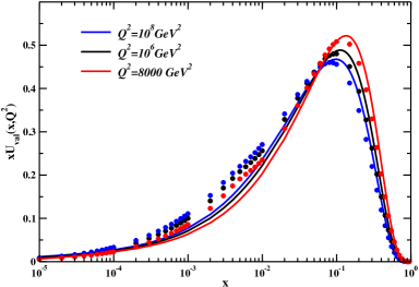
Figure 1: The $xU_{val}(x,\,Q)$ valance quark distributions in different values of $Q^{2}$ in comparison with APFEL model.

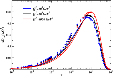
Figure 2: The $xD_{val}(x,\,Q^{2})$ valance quark distributions in different values of $Q^{2}$ in comparison with APFEL model.

The comparison photon distribution function, $x\gamma(x,Q^{2})$, gloun distribution function, $xg(x,Q^{2})$,with APFEL and CT14QED models at $Q^{2}=10^{4}GeV^{2}$ for $\alpha_{s}(Q^{2}=M_{z}^{2})=0.118$ is well demonstrated in Fig. 3. This plot indicates that our results are in good agreement with APFEL and CT14QED models. Also it is clear from this figure for photon distribution function that our results in comparison with the CT14QED photon distribution function are very similar at large value of x and are different for small value of x. We also investigate the effect of an increasing in value of $Q^{2}>Q_{0}^{2}$ on the photon distribution functions and conclude that the CT14QED photon distribution function becomes large, whereas our results is distinctly different and much smaller at small values of x ( Corresponding plot omitted for briefly).

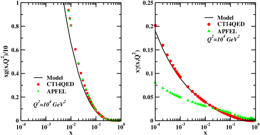
Figure 3: The photon and gloun distribution functions at $Q^{2}=10^{4}GeV^{2}$as a function of x in LO QED and NLO QCD approximations in comparison with the available APFEL and CT14QED models.

In figure  4 we displayed the valance quark distributions at scale of $Q^{2}=10^{4}GeV^{2}$. we compared those with the APFEL and CT14QED models. It is shown that with increasing the value of $Q^{2}$, the contribution of valence quarks are decreased. Therefore, we can conclude the photon contribution is now significantly considerable.

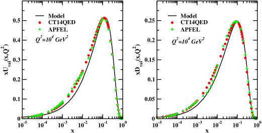
Figure 4: The comparison valance quark distributions at $Q^{2}=10^{4}GeV^{2}$ as a function of x with the availabe CT14QED and APFEL models.

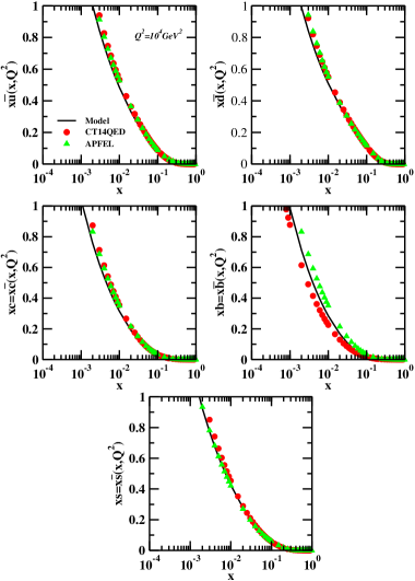
Figure 5: The comparison sea quark distributions at $Q^{2}=10^{4}GeV^{2}$as a function of x in LO QED and NLO QCD approximations with the availabe CT14QED and APFEL models.

Fig.  5 displays our analytical sea quark distribution functions at $Q^{2}=10^{4}GeV^{2}$. We compared our results with the newly released PDFs global parameterizations from CT14QED  [6] and APFEL model. The CT14QED, is the first set of CT14 parton distribution functions obtained by including QED evolution at leading order with next-to-leading order QCD evolution in their global analysis.

It is found that the sea quark distribution functions in comparison with the photon distribution function in the large values of x with increasing the value of $Q^{2}$, contribution of photon is most significant. It may also be noted that in range of high x the photon distribution function is larger than the bottom quark distribution function as increasing the value of $Q^{2}$.

It is observed from these figures with increasing the value of $Q^{2}$ that the parton distribution functions decrease for the large values of x and increase for the small values of x.

We now proceed by calculating proton structure function. Our aim of to investigate the proton structure function is to compare our results with a physical observable that confirm the correctness of our analytical solutions. The Laplace transform technique is also applied to the proton structure function, $F_{2}^{p}(x,Q^{2})$, which leads to an analytical solution for this function. The method illustrated in this analysis enable us to achieve strictly analytical solution for proton structure function in terms of x variable.

We will yield the total proton structure functions as $F_{2}^{p,total}(x,Q^{2})=F_{2}^{p,light}(x,Q^{2})+F_{2}^{heavy}(x,Q^{2})$ where $F_{2}^{heavy}(x,Q^{2})=F_{2}^{c}(x,Q^{2})+F_{2}^{b}(x,Q^{2})$ are the charm and bottom quarks structure functions.

For light quarks, the proton structure function $F_{2}^{p,light}(x,Q^{2})$ in Laplace s space, up to the next-to-leading order approximation is given by

$$F_{2}^{p,light}(s,\tau)=F_{2}^{NS}(s,\tau)+F_{2}^{S}(s,\tau)+F_{2}^{G}(s,\tau),$$ (35)

where the non-singlet $F_{2}^{NS}$, singlet $F_{2}^{S}$ and gloun $F_{2}^{G}$ contributions are written as

$$F_{2}^{NS}(s,\tau)=(\frac{4}{9}u_{v}(s,\tau)+\frac{1}{9}d_{v}(s,\tau))(1+\frac{\tau}{2\pi}C_{q}^{(1)}(s))$$

$$F_{2}^{S}(s,\tau)=(\frac{4}{9}2\bar{u}(s,\tau)+\frac{1}{9}2\bar{d}(s,\tau)+\frac{1}{9}2\bar{s}(s,\tau))(1+\frac{\tau}{2\pi}C_{q}^{(1)}(s))$$

$$F_{2}^{G}s,\tau)=(\frac{4}{9}+\frac{1}{9}+\frac{1}{9})g(s,\tau)(\frac{\tau}{2\pi}C_{g}^{(1)}(s))$$ (36)

where the $C_{q}^{(1)}(s)$ and $C_{g}^{(1)}(s)$ are the next-to-leading order Wilson coefficient functions, derived in Laplace s space by $C_{q}(s)=L[e^{\text{\textminus}\nu}c_{q}(e^{\text{\textminus}\nu});s]$ and $C_{g}(s)=L[e^{-\nu}c_{g}(e^{-\nu});s]$. The next-to-leading order Wilson coefficient functions in Bjorken x space are found in refs.  [27]. We have found the final desired solution of the proton structure function in x space, $F_{2}^{p,light}(x,Q^{2})$, using the inverse Laplace transform and the appropriate change of variables.

The next-to-leading order contribution of heavy quarks, $F_{2}^{c,b}(x,Q^{2})$, to the proton structure function can be calculated in the fixed flavour number scheme (FFNS) approach  [16, 29, 30, 31, 32, 33, 34].

The heavy quarks structure function, $F_{2}^{c,b}(x,Q^{2})=F_{2}^{(nl)}(x,Q^{2})+F_{2}^{(d)}(x,Q^{2})$, where $F_{2}^{(nl)}(x,Q^{2})$ and $F_{2}^{(d)}(x,Q^{2})$ are the massive-scheme heavy-quark structure function and the “difference” contribution, respectively. The Laplace Transforms of $F_{2}^{(nl)}(x,Q^{2})$ and $F_{2}^{(d)}(x,Q^{2})$ for charm and bottom quarks, are given by

$$F_{2}^{(nl)}(s,\tau)=\frac{4}{9}\tau\left(C_{g}^{(1)}(s)\>Log\left(\frac{Q^{2}}{m_{c}^{2}}\right)+C_{g}^{(1)}(s)\right)g(s,\tau)$$ (37)

$$F_{2}^{(d)}(s,\tau)=\frac{4}{9}\left(1+\frac{\tau}{2\pi}C_{q}^{(1)}(s)\right)(c(s,\tau)+\bar{c}(s,\tau))+\frac{4}{9}\frac{\tau}{2\pi}(C_{g}^{(1)}(s)-C_{g}^{(1)}(s,m_{c}^{2}))\,g(s,\tau)$$ (38)

and

$$F_{2}^{(nl)}(s,\tau)=\frac{1}{9}\tau\\ \left(C_{g}^{(1)}(s)\>Log\left(\frac{Q^{2}}{m_{b}^{2}}\right)+C_{g}^{(1)}(s)\right)g(s,\tau)$$ (39)

$$F_{2}^{(d)}(s,\tau)=\frac{1}{9}\left(1+\frac{\tau}{2\pi}C_{q}^{(1)}(s)\right)(b(s,\tau)+\bar{b}(s,\tau))\\ +\frac{1}{9}\frac{\tau}{2\pi}(C_{g}^{(1)}(s)-C_{g}^{(1)}(s,m_{b}^{2}))\,g(s,\tau)$$ (40)

where $m_{c}$ and $m_{b}$ are the charm and bottom quark masses. The coefficient functions $C_{g}^{(1)}(s,m_{c}^{2})$ and $C_{g}^{(1)}(s,m_{b}^{2})$ are found in ref. [35].

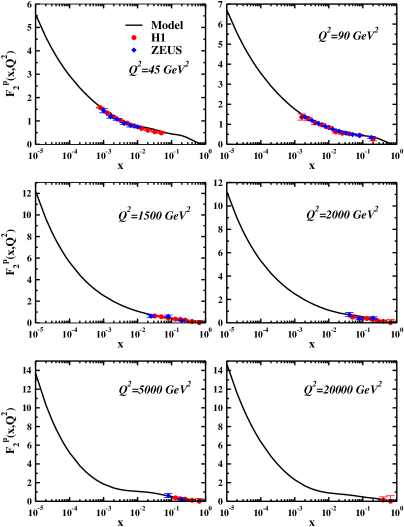
Figure 6: The proton structure function at $Q^{2}=45,\,90,\,1500,\,2000\,,5000\>and\>20000\>GeV^{2}$ in comparison with experimental data.

Figure 6 depicts the comparison the proton structure function with the corresponding available experimental data from the H1 and ZEUS Collaborations in the several values of $Q^{2}$. The results demonstrate that there are good agreement between them. It is clear that the proton structure function increases with an increase in value of $Q^{2}$ for small values of x and decrease for large values of x. All figures indicate that the analytical solutions work well beyond the charm quark mass threshold, $Q^{2}>Q_{0}^{2}(\approx m_{c}^{2}=1.677\,GeV^{2})$. Figure 7 displays the comparison the proton structure function with QED corrections and without this corrections (QCD analysis) with the corresponding experimental data from the H1 Collaborations in the value of $Q^{2}=12000\,GeV^{2}$. This figure shows that the proton structure function with QED corrections in good agreement with experimental data in the high energy.

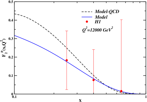
Figure 7: The proton structure function at $Q^{2}=12000GeV^{2}$in comparison with QCD analysis and experimental data

4 CONCLUSIONS

In this paper, we utilized the Laplace transform technique to calculate the Laplace transformation of splitting functions and extract the parton distribution functions of quark, antiquark, gloun and photon inside the proton. Our calculations are done in LO QED and NLO QCD approximations. We finally extracted the unpolarized proton structure functions at the different values of $Q^{2}$. Our results are compared with APFEL and newly released CT14QED codes and also with experimental data which indicate good agreements between them. To determine the proton structure function at any arbitrary $Q^{2}$ scale , we only need to know the initial distributions for singlet, gluon, non-singlet and photon distributions at the input scale of $Q_{0}^{2}$. We borrowed the initial inputs from CT14QED code at $Q_{0}=1.295\,GeV$ to be sure about the correctness of our solutions. The solutions are seem to be correct because the parton distribution functions and the proton structure function have good agreement with those from all global parameterizations (as well as CT14QED) and experimental data. In the future work with a global parameterization we can determine these initial inputs. These PDFs can specifically design for use in precision cross section predictions and uncertainties at the LHC.

ACKNOWLEDGMENT

We would like to thank Professor S. Atashbar Tehrani for his help and for the productive discussions.

APPENDIX: MATHEMATICA PROGRAM OF THE SPLITTING FUNCTIONS

Program containing our results for the Laplace transforms of the splitting functions at LO QED and NLO QCD approximations can be obtained via Email from the authors upon request.

References

- [1] G. Aad et al. [ATLAS Collaboration], Phys. Lett. B 725, 223 (2013) doi:10.1016/j.physletb.2013.07.049 [arXiv:1305.4192 [hep-ex]].
- [2] A. D. Martin, R. G. Roberts, W. J. Stirling and R. S. Thorne, Eur. Phys. J. C 4, 463 (1998) doi:10.1007/s100529800904, 10.1007/s100520050220 [hep-ph/9803445].
- [3] A. D. Martin, R. G. Roberts, W. J. Stirling and R. S. Thorne, Eur. Phys. J. C 39, 155 (2005) doi:10.1140/epjc/s2004-02088-7 [hep-ph/0411040].
- [4] V. Bertone, S. Carrazza and J. Rojo, Comput. Phys. Commun. 185, 1647 (2014) doi:10.1016/j.cpc.2014.03.007 [arXiv:1310.1394 [hep-ph]].
- [5] R. D. Ball et al. [NNPDF Collaboration], Nucl. Phys. B 877, 290 (2013) doi:10.1016/j.nuclphysb.2013.10.010 [arXiv:1308.0598 [hep-ph]].
- [6] C. Schmidt, J. Pumplin, D. Stump and C. P. Yuan, Phys. Rev. D 93, no. 11, 114015 (2016) doi:10.1103/PhysRevD.93.114015 [arXiv:1509.02905 [hep-ph]].
- [7] M. M. Block, L. Durand and D. W. McKay, Phys. Rev. D 77, 094003 (2008) doi:10.1103/PhysRevD.77.094003 [arXiv:0710.3212 [hep-ph]].
- [8] M. M. Block, L. Durand, P. Ha and D. W. McKay, Eur. Phys. J. C 69, 425 (2010) doi:10.1140/epjc/s10052-010-1413-4 [arXiv:1005.2556 [hep-ph]].
- [9] M. M. Block, L. Durand, P. Ha and D. W. McKay, Phys. Rev. D 84, 094010 (2011) doi:10.1103/PhysRevD.84.094010 [arXiv:1108.1232 [hep-ph]].
- [10] M. M. Block, L. Durand, P. Ha and D. W. McKay, Phys. Rev. D 83, 054009 (2011) doi:10.1103/PhysRevD.83.054009 [arXiv:1010.2486 [hep-ph]].
- [11] M. M. Block, Eur. Phys. J. C 65, 1 (2010) doi:10.1140/epjc/s10052-009-1195-8 [arXiv:0907.4790 [hep-ph]].
- [12] M. M. Block, Eur. Phys. J. C 68, 683 (2010) doi:10.1140/epjc/s10052-010-1374-7 [arXiv:1004.3585 [hep-ph]].
- [13] M. M. Block and L. Durand, Eur. Phys. J. C 71, 1806 (2011) doi:10.1140/epjc/s10052-011-1806-z [arXiv:1108.5492 [math.NA]].
- [14] H. Khanpour, A. Mirjalili and S. Atashbar Tehrani, Phys. Rev. C 95, no. 3, 035201 (2017) doi:10.1103/PhysRevC.95.035201 [arXiv:1601.03508 [hep-ph]].
- [15] H. Khanpour, A. N. Khorramian and S. A. Tehrani, J. Phys. G 40, 045002 (2013) doi:10.1088/0954-3899/40/4/045002 [arXiv:1205.5194 [hep-ph]].
- [16] M. Gluck, P. Jimenez-Delgado and E. Reya, Eur. Phys. J. C 53, 355 (2008) doi:10.1140/epjc/s10052-007-0462-9 [arXiv:0709.0614 [hep-ph]].
- [17] F. Taghavi-Shahri, A. Mirjalili and M. M. Yazdanpanah, Eur. Phys. J. C 71, 1590 (2011) doi:10.1140/epjc/s10052-011-1590-9 [arXiv:1005.4786 [hep-ph]].
- [18] S. Atashbar Tehrani, F. Taghavi-Shahri, A. Mirjalili and M. M. Yazdanpanah, Phys. Rev. D 87, no. 11, 114012 (2013) Erratum: [Phys. Rev. D 88, no. 3, 039902 (2013)]. doi:10.1103/PhysRevD.87.114012, 10.1103/PhysRevD.88.039902
- [19] M. Zarei, F. Taghavi-Shahri, S. Atashbar Tehrani and M. Sarbishei, Phys. Rev. D 92, no. 7, 074046 (2015) doi:10.1103/PhysRevD.92.074046 [arXiv:1601.02815 [hep-ph]].
- [20] I. I. Balitsky and L. N. Lipatov, Sov. J. Nucl. Phys. 28, 822 (1978) [Yad. Fiz. 28, 1597 (1978)].
- [21] G. Altarelli and G. Parisi, Nucl. Phys. B 126, 298 (1977). doi:10.1016/0550-3213(77)90384-4
- [22] S. Carrazza, arXiv:1509.00209 [hep-ph].
- [23] A. Deur, S. J. Brodsky and G. F. de Teramond, Prog. Part. Nucl. Phys. 90, 1 (2016) doi:10.1016/j.ppnp.2016.04.003 [arXiv:1604.08082 [hep-ph]].
- [24] W. Furmanski and R. Petronzio, Phys. Lett. 97B, 437 (1980). doi:10.1016/0370-2693(80)90636-X
- [25] G. Curci, W. Furmanski and R. Petronzio, Nucl. Phys. B 175, 27 (1980). doi:10.1016/0550-3213(80)90003-6
- [26] M. Roth and S. Weinzierl, Phys. Lett. B 590, 190 (2004) doi:10.1016/j.physletb.2004.04.009 [hep-ph/0403200].
- [27] W. A. Bardeen, A. J. Buras, D. W. Duke and T. Muta, Phys. Rev. D 18, 3998 (1978). doi:10.1103/PhysRevD.18.3998
- [28] M. Gluck, C. Pisano and E. Reya, Eur. Phys. J. C 50, 29 (2007) doi:10.1140/epjc/s10052-006-0189-z [hep-ph/0610060].
- [29] M. Gluck, C. Pisano and E. Reya, Eur. Phys. J. C 40, 515 (2005) doi:10.1140/epjc/s2005-02167-3 [hep-ph/0412049].
- [30] M. Gluck, P. Jimenez-Delgado, E. Reya and C. Schuck, Phys. Lett. B 664, 133 (2008) doi:10.1016/j.physletb.2008.04.063 [arXiv:0801.3618 [hep-ph]].
- [31] M. Gluck, E. Reya and M. Stratmann, Nucl. Phys. B 422, 37 (1994). doi:10.1016/0550-3213(94)00131-6
- [32] E. Laenen, S. Riemersma, J. Smith and W. L. van Neerven, Phys. Lett. B 291, 325 (1992). doi:10.1016/0370-2693(92)91053-C
- [33] S. Riemersma, J. Smith and W. L. van Neerven, Phys. Lett. B 347, 143 (1995) doi:10.1016/0370-2693(95)00036-K [hep-ph/9411431].
- [34] E. Laenen, S. Riemersma, J. Smith and W. L. van Neerven, Nucl. Phys. B 392, 162 (1993). doi:10.1016/0550-3213(93)90201-Y
- [35] S. Forte, E. Laenen, P. Nason and J. Rojo, Nucl. Phys. B 834, 116 (2010) doi:10.1016/j.nuclphysb.2010.03.014 [arXiv:1001.2312 [hep-ph]].