On the Propagation of a Geoeffective Coronal Mass Ejection during March 15 – 17, 2015
Abstract
The largest geomagnetic storm so far in the solar cycle 24 was produced by a fast coronal mass ejection (CME) originating on 2015 March 15. It was an initially west-oriented CME and expected to only cause a weak geomagnetic disturbance. Why did this CME finally cause such a large geomagnetic storm? We try to find some clues by investigating its propagation from the Sun to 1 AU. First, we reconstruct the CME’s kinematic properties in the corona from the SOHO and SDO imaging data with the aid of the graduated cylindrical shell (GCS) model. It is suggested that the CME propagated to the west away from the Sun-Earth line with a speed of about 817 km s-1 before leaving the field of view of the SOHO/LASCO C3 camera. A magnetic cloud (MC) corresponding to this CME was measured in-situ by the Wind spacecraft two days after the CME left LASCO’s field of view. By applying two MC reconstruction methods, we infer the configuration of the MC as well as some kinematic information, which implies that the CME possibly experienced an eastward deflection on its way to 1 AU. However, due to the lack of observations from the STEREO spacecraft, the CME’s kinematic evolution in interplanetary space is not clear. In order to fill this gap, we utilize numerical MHD simulation, drag-based CME propagation model (DBM) and the model for CME deflection in interplanetary space (DIPS) to recover the propagation process, especially the trajectory, of the CME from to 1 AU under the constraints of the derived CME’s kinematics near the Sun and at 1 AU. It is suggested that the trajectory of the CME was deflected toward the Earth by about , consistent with the implication from the MC reconstruction at 1 AU. This eastward deflection probably contributed to the CME’s unexpected geoeffectiveness by pushing the center of the initially west-oriented CME closer to the Earth.
WANG ET AL. \titlerunningheadCME Deflection
1 Introduction
As the most important driver of severe space weather, coronal mass ejections (CMEs) and their geoeffectiveness have been studied intensively. Previous statistical studies have shown that not all the front-side halo CMEs are geoeffective (e.g., Webb et al., 2001; Wang et al., 2002; Zhao and Webb, 2003; Yermolaev et al., 2005), and not all non-recurrent geomagnetic storms can be tracked back to a CME (e.g., Cane et al., 2000; Cane and Richardson, 2003; Yermolaev et al., 2005; Zhang et al., 2007). These phenomena may cause some failed predictions of the geoeffectiveness of CMEs. The recent notable event exhibiting such a failure was on 2015 March 15 when a fast CME originated from the west hemisphere. Space Weather Prediction Center (SWPC) of NOAA initially forecasted that the CME would at most cause a very minor geomagnetic disturbance labeled as G1, a scale used by SWPC to measure the intensity of geomagnetic storms. However, the CME produced the largest geomagnetic storm so far, at G4 level with the provisional value of nT, in the current solar cycle 24 (Kataoka et al., 2015; Wood et al., 2016). The major geomagnetic storm was called the “2015 St. Patrick’s Day” event as its main phase and peak occurred on March 17, and the surprising CME was selected as a campaign event by International Study of Earth-affecting Solar Transients (ISEST)111http://solar.gmu.edu/heliophysics/index.php/03/17/2015_04:00:00_UTC, a program under SCOSTEP, and also by Coupling, Energetics and Dynamics of Atmospheric Regions (CEDAR)222http://cedarweb.vsp.ucar.edu/wiki/index.php/2015_Workshop:The_March_17_2015_great_storm.
Such an unexpected phenomenon naturally raises the first question for the forecasting of the geoeffectiveness of a CME, i.e., whether or not a CME will hit the Earth even though we know the source location and initial kinematic properties of the CME. A full understanding of the propagation trajectory of a CME from the Sun to 1 AU is the key to this question. Of course, it is not the only factor determining the geoeffectiveness of a CME. The magnetic field strength and the orientation of the CME flux rope, which directly affect the strength and duration of the interval of the south-component of the magnetic field, is also important for determining its geoeffectiveness.
It has been well accepted that the CME’s trajectory can be deflected in the corona (within a few tens of solar radii, ). Wang et al. (2011) illustrated that such deflections can be classified into three types: asymmetrical expansion, non-radial ejection and deflected propagation. In a statistical sense, CMEs tend to be deflected toward the equator during solar minimum (e.g., MacQueen et al., 1986; Cremades and Bothmer, 2004; Wang et al., 2011) or deflected away from coronal holes (e.g., Gopalswamy et al., 2003, 2009; Cremades et al., 2006). The physics behind these deflections is that the gradient of the magnetic energy density may cause the CME to move toward the place where the magnetic energy density reaches the minimum, usually the location of the heliospheric current sheet (Shen et al., 2011a; Gui et al., 2011; Zuccarello et al., 2012; Isavnin et al., 2013; Kay et al., 2013). Although the CME’s deflection in the corona could be tens of degrees and may change the geoeffectiveness of a CME, it still can be monitored by coronagraphs (e.g., Möstl et al., 2015). Thus, the possible deflection of a CME in interplanetary space rather than the deflection in the corona is one of the major sources of uncertainty in the prediction of the CME impact at the Earth.
The possibility of the CME deflection in interplanetary space was first proposed by Wang et al. (2004). They suggested that, different from the deflection in the corona, the CME’s trajectory in interplanetary space could be deflected due to the velocity difference between the CME and the ambient solar wind. For a fast CME, the solar wind plasma and interplanetary magnetic field will be piled up from the west and ahead of it, leading to a net deflection force toward the east; for a slow CME, the picture is the opposite. A kinematic model (called DIPS, Deflection in InterPlanetary Space, hereafter) was therefore developed (Wang et al., 2004). Such deflections are thought to be gradual and much slower than that in the corona, but the total amount of the deflection angle is comparable to that in the corona as it takes place over a much longer distance. Such evidence can also be found in previous studies (e.g., Wang et al., 2002, 2004, 2006; Kilpua et al., 2009; Lugaz et al., 2010; Isavnin et al., 2014; Kay and Opher, 2015). One of the most comprehensive analysis of the CME’s trajectory in interplanetary space was done by Wang et al. (2014) for a slow CME, which was proven to experience a westward deflection all the way from the corona to 1 AU with a total deflection angle of more than 20 degrees.
For the 2015 March 15 CME, there were no STEREO (Solar TErrestrial RElations Observatory, Kaiser et al., 2008) data as the twin spacecraft were behind the Sun and not taking images. All the information of the CME came from the remote-sensing data provided by the Solar and Heliospheric Observatory (SOHO) and the in-situ data by Wind (or ACE) spacecraft at 1 AU. The interplanetary space between the corona to 1 AU thus had an observational gap, and therefore the propagation of the CME from the Sun to 1 AU is unclear. In this paper, we try to recover the kinematic evolution of the CME from the limited observations and fill the gap with the aid of models. We particularly focus on the trajectory of the CME to demonstrate how the CME behavior in interplanetary space favors its strong geoeffectiveness.
2 Kinematics of the CME in the corona
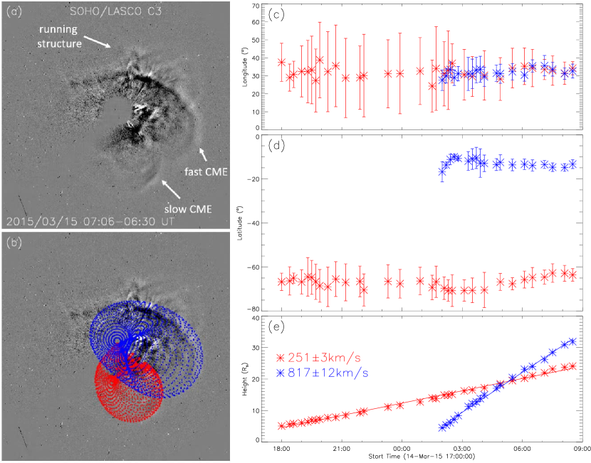
The fast CME of interest first appeared in the field of view (FOV) of LASCO (Large Angle and Spectrometric Coronagraph, Brueckner et al., 1995) C2 camera on board the SOHO on March 15 at about 01:36 UT, and left the FOV of LASCO/C3, which monitors the corona within 30 , around 09 UT. It was a partial halo CME with most material ejected toward the west as shown in Figure 1a.
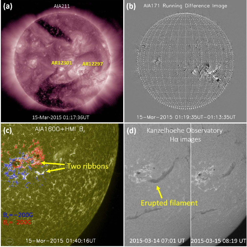
By examining the solar EUV images, e.g., Figure 2a and 2b, taken by the Atmospheric Imaging Assembly (AIA, Lemen et al., 2012) on board the Solar Dynamics Observatory (SDO), we can identify that the source region of the CME is active region (AR) 12297 on the west hemisphere of the Sun with a large coronal hole (CH) to the south-east of it. The eruption took place around the location of W35S15 with filament-like material moving toward the south-west direction. Meanwhile, two bright ribbons can be seen in the AIA 1600Å passband (Fig.2c), suggesting a typical eruptive flare. The two daily images taken by Kanzelhoehe Observatory before and after the eruption (Fig.2d) did show a disappearance of a segment of a thick filament near the AR. However, as will be discussed below, there was another slow CME perhaps originating from the same AR between the times of the two images. Thus, the association of the disappeared filament segment in the images to the CME is unclear. The AIA EUV images suggest a clear filament eruption during the fast CME, and therefore it is very likely that the disappeared filament is associated with this CME. Considering that the filament is a good tracer of the CME flux rope, one may estimate that the tilt angle, i.e., the angle between the main axis of the CME flux rope and the solar equator, is initially within the range of .
It should be noted that the coronal conditions during the fast CME traveling through the LASCO FOVs were complicated. The movie (see supplementary material) made from the SOHO/LASCO images (or see the example image Fig.1a) reveals that (1) there was a structure running faster than the fast CME along the north-west direction, and (2) there was a slow CME, which was launched earlier on March 14, propagating toward the south. The running structure appeared in the LASCO FOV at the same time as the fast CME appeared. It not only ran faster than but also looked fainter than the fast CME. This running structure might be the shock wave driven by the fast CME, or an independent magnetic structure that erupted from the Sun. We incline to the latter because the running structure was much faster than the fast CME and its shape was much narrow than and different from the CME’s front. However, near the eruption of the fast CME, we cannot find any other notable eruption signatures on the visible solar disk. Although stealth CMEs exist, they tend to be slow (e.g., Robbrecht et al., 2009; Wang et al., 2011; Howard and Harrison, 2013). Thus, the fast running structure was probably a real ejection from the backside of the Sun. Since the structure propagated faster than and ahead of the CME of interest, we do not consider any possible interaction between them.
For the preceding slow CME, there are two possibilities of its source locations (due to the lack of STEREO observations). One was suggested by Gopalswamy and Yashiro at the ISEST workshop in October, 2015. They thought that it was a backside event because the pre-existing streamer disturbed by the slow CME was moving to the south pole, suggesting that its location was on the backside. The other possibility is that it was a front-side CME. There was a notable eruptive signature in the same AR 12297 around 12:00 UT on March 14. The time and location match well with the appearance and the speed of the slow CME in the LASCO/C2 FOV. If the first possibility was true, there should be no interaction between the slow CME and the fast CME of interest. But if the second possibility was true, the two CMEs might have interacted with each other.
With the aid of foward modeling, e.g., the GCS model (Thernisien et al., 2009; Thernisien, 2011), we then analyze the kinematics of the two CMEs as well as this possible interaction. Since SOHO/LASCO provides only one angle of view, the GCS fitting suffers from a larger uncertainty than that when the STEREO data are available. Thus, we reduce the degrees of freedom during the fitting by setting three free parameters, the tilt angle, aspect ratio and angular width, to be constant, and only vary the other three free parameters, the longitude, latitude and the height. Thanks to a sufficient number of images in the time sequence, these free parameters of the GCS model can still be roughly constrained by trial and error. The uncertainties in these parameters are estimated by following the method of Thernisien et al. (2009), i.e., by decreasing the goodness-of-fit between the leading edge of the CME and the model by 10%. Since the leading edge of the CME in all the images is determined manually by hand-clicks, which may increase the errors, the uncertainties inferred by the above method are underestimated. For the fast CME, the best value of the tilt angle is about , the aspect ratio about 0.66, and the angular width about (edge-on) or (face-on). For the preceding slow CME, they are , 0.47, and , respectively. The uncertainties in the tilt angle, aspect ratio and the angular width are about , 0.12 and . These uncertainties are very large, and thus these fitting values are only used for reference.
For the other three time-dependent parameters, the fitting results are shown in Figure 1c–1e. The uncertainty in the longitude is about , that in the latitude is better, about , and that in the height is less than one solar radius. The two CMEs almost propagated along the same longitude, which is around , but in latitude, the two CMEs were separated by about . Considering the angular width of the two CMEs, they might marginally interact with each other if the preceding slow CME was a front-side event. According to the height-time plot shown in Figure 1e, the two CMEs traveled through the LASCO FOVs at a speed of 817 and 251 km s-1, respectively. The leading edge of the fast CME caught up with the leading edge of the preceding slow one around 05:20 UT. Thus, the possible interaction should start around 03:00 UT and end before the fast CME left the FOV of LASCO/C3. However, neither considerable acceleration of the preceding slow CME nor deceleration of the fast CME can be found in the height-time profiles. An interesting phenomenon is that the preceding slow CME was systematically deflected toward lower latitude, and the fast CME slightly toward higher latitude. Due to the significant uncertainties, we cannot conclude that the two CMEs interacted based on such small deflections. Nevertheless, we can conclude that the two CMEs at most experienced a very weak interaction, which has little influence on the kinematics of the fast CME in interplanetary space. Note, there is also a great possibility that the two CMEs did not interact at all, because the preceding one might come from the backside of the solar disk.
The inferred kinematic evolution of the two CMEs in the corona suggest that the fast CME should be able to encounter the Earth but the slow CME is unlikely to encounter the Earth. Since the fast CME may drive a shock at front, what we fitted with GCS model is probably not the leading edge of its flux rope but the driven shock. The recent work by Good and Forsyth (2016) suggested that the longitudinal extent of the flux rope carried by a CME is typically about , smaller than its driven shock if any. Thus, the angular width of the fast CME derived from the GCS model is probably overestimated. If this were the case, the fast CME’s flux rope might just graze the Earth with a weaker geoeffectiveness.
3 In-situ observations at 1 AU
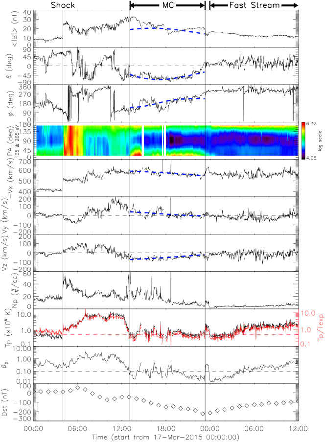
Two days later, a fast forward shock followed by a magnetic cloud (MC) was recorded by the Wind spacecraft (Lepping et al., 1995; Ogilvie et al., 1995; Lin et al., 1995) as shown in Figure 3. The shock arrived at 1 AU at 04:00 UT on March 17. Its driver, the MC, occurred between 13:05 and 23:20 UT, and is characterised by the reduced fluctuation in the magnetic field, the large and smooth rotation of the magnetic field direction, evident bi-directional suprathermal electron beams and the low temperature and proton . According to the classification proposed by Bothmer and Schwenn (1998) and Mulligan et al. (1998), the MC is an ESW-type flux rope. A fast stream, probably from the CH (as seen in Fig.2a), was catching up with the MC, causing an interaction region during 23:20 – 23:55 UT, when the density and temperature were enhanced, the magnetic field strength reduced and the magnetic field rotation ceased. Our identification of the MC is the same as that by Kataoka et al. (2015). The MC and the shock sheath ahead of it caused a double-peak major geomagnetic storm with the provisional value of nT (see the last panel of Fig.3).
The MC is the interplanetary counterpart of the CME originating on March 15 because of the following two reasons. (1) If the MC corresponds to the CME, the transit time of the CME from its first appearance in the LASCO/C2 and the arrival at 1 AU is about 59.5 hours, and the average transit speed is about 690 km s-1, which is consistent with the CME speed, 817 km s-1, in the FOV of LASCO/C3 and the measured MC speed, km s-1, at 1 AU. (2) Except for the preceding slow CME mentioned in the last section, there was no other CME candidate during March 14 – 16 responsible for the MC according to the LASCO observations. The slow CME propagated far away from the ecliptic plane and was probably on the other side of the Sun. Thus, it should not be detected near the Earth. It should be noted that Liu et al. (2015) also analyzed this event and proposed a different scenario that there were two interplanetary CMEs (ICMEs), corresponding to the slow and fast CMEs on March 14 and 15, respectively, and the main ICME, i.e., the one corresponding to the fast CME, was identified in the interval from about 18 UT on March 17 to 16 UT on the next day. This interpretation is not in agreement with our above analysis. The Wind data shown in Figure 3 reveal that the smooth rotation of magnetic field vector and the bi-directional electron streams ceased at the end of March 17.
There are various models developed to reconstruct MCs from one-dimensional in-situ data, including cylindrically symmetrical force-free flux rope models (e.g., Goldstein, 1983; Marubashi, 1986; Burlaga, 1988; Lepping et al., 1990; Wang et al., 2015), asymmetrically cylindrical (non)force-free flux rope models (e.g., Mulligan and Russell, 2001; Hu and Sonnerup, 2002; Hidalgo et al., 2002; Cid et al., 2002; Vandas and Romashets, 2003) and torus-shaped flux rope models (e.g., Romashets and Vandas, 2003; Marubashi and Lepping, 2007; Hidalgo and Nieves-Chinchilla, 2012). Here we use the velocity-modified cylindrical force-free flux rope (VFR) model, which considers the propagation and expansion of a MC as well as the plasma poloidal motion inside the MC (Wang et al., 2015), to fit the MC. In this model, the magnetic field is described by the Lundquist solution, and the velocity is incorporated under the assumptions of self-similar evolution and magnetic flux conservation. This model is proven to yield similar results as the cylindrically symmetrical force-free flux rope model by Lepping et al. (1990). We choose this model because the fitting results contain some kinematic information of the CME, which may provide some clues on the trajectory of the CME in interplanetary space. In addition, we also apply the Grad-Shafranov (GS) reconstruction technique (Hu and Sonnerup, 2002) to the MC to see the similarity and difference between the model results.
| Model | |||||||||||
|---|---|---|---|---|---|---|---|---|---|---|---|
| (1) | (2) | (3) | (4) | (5) | (6) | (7) | (8) | (9) | (10) | (11) | (12) |
| VFR | 32 | 0.09 | 59 | 51 | 45 | ||||||
| GS | / | / | / | / | / |
From the left to the right, the columns give (1) the model used to derive the parameters, (2) the magnetic field strength at the MC’s axis in units of nT, (3) the radius of the MC in units of AU, (4) the elevation angle of the MC’s axis in the GSE coordinates, (5) the azimuthal angle of the MC’s axis in the GSE coordinates, (6) the handedness of the MC, (7) the closest approach of the observational path to the MC’s axis, (8–10) the propagation velocity of the MC in the GSE coordinates in units of km s-1, (11) the expansion speed of the MC in units of km s-1 and (12) the poloidal speed of the MC plasma in units of km s-1.
The best-fit values of the free parameters of the VFR model for the MC of interest are given in Table 1, and the fitting curves are plotted as the dashed blue lines in Figure 3, which match the observed profiles fairly well in both magnetic field and velocity. In particular, we highlight the following parameters: (i) Sign of the helicity or handedness of the MC is , which obeys the pattern that the southern hemisphere of the Sun usually accumulates positive helicity (e.g., Rust and Kumar, 1996). (ii) Closest approach is , where is the radius of the MC, indicating that the observational path is far away from the MC’s axis. (iii) Orientation of the MC’s axis is and in GSE coordinates, corresponding to a tilt angle of about when projected on the plane-of-the-sky. Considering that the magnetic polarity in the CME source region is negative/positive on the southern/northern side of the filament associated with the CME (see Fig.2c) and the helicity of the MC is positive, this value is close to the CME’s tilt angle of estimated from the GCS fitting. The orientation also suggests that the angle between the axis of the observed portion of the MC and the Sun-Earth line is about , meaning that the flank of the MC was passed through (e.g., Janvier et al., 2013). (iv) Combination of (i) and (iii) gives how the magnetic field lines wind in the MC, which is in agreement with the distribution of the magnetic field polarities in the CME source region, i.e., positive/negative polarity region on the north-west/south-east side of the associated filament (Fig.2c).
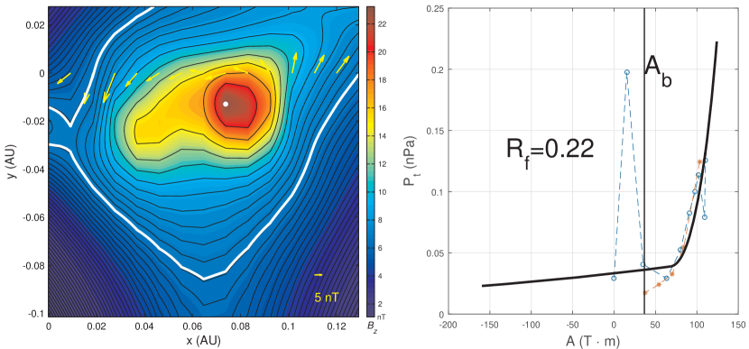
The results of the GS reconstruction are shown in Figure 4 and the fitting parameters are listed in Table 1 too. It is a substantially different technique from the VFR fitting which is a type of forward models. The GS reconstruction neither presets the shape of the flux rope nor assumes a fore-free state, but uses the GS equation to infer the two and a half dimensional distribution of magnetic field at the cross-section of the flux rope from the observed magnetic field and thermal pressure along the spacecraft path under the assumption of being time-stationary and magnetohydrostatic. The fitting of , the sum of the axial magnetic pressure and the thermal pressure, which is essential to the GS reconstruction, yields a residue (Hu et al., 2004) as a measure of goodness of fit. As judged from the right panel of Figure 4, the interpretation of a flux-rope configuration shown in the left panel is valid for the limited region within the white contour line and under the assumption that significant axial current exists at the center. The GS reconstruction gives the same handedness as VFR model, and we can read from Figure 4 that the magnetic field at the center is about 23 nT and the radius about 0.08 AU in -axis or 0.05 AU in -axis, slightly smaller than but comparable to those derived from the VFR model. The closest approach is about AU. For the orientation, the GS model is quite consistent with the VFR model in the elevation angle, but deviates significantly in the azimuthal angle. The angle between the orientations of the GS model and the VFR model is about , the largest inconsistency between the two models. The comparison suggests that the solution of the fit to the in-situ measurements is not unique. The most sensitive parameter is the orientation of the flux rope axis. Besides, the selection of the boundaries of a MC might also significantly affect the fitting results (private communication with K. Marubashi and Q. Hu). It is difficult to evaluate which one is more reliable. We list the two possible solutions here for reference and also to raise the question for further attention.
Riley et al. (2004) performed ‘blind tests’ by applying five different fitting techniques, including the cylindrical linear force-free flux rope model, the elliptical cross-section non-force-free flux rope model and the GS model, to a MHD simulated MC. The largest deviation among these model results is in the orientation, especially when the observational path is far away from the MC’s axis. The March 17 MC encountered the Earth with the closest approach of , falling into this scenario. Thus, it is not surprising that we get quite different results in the orientation from the different models. However, the tests by Riley et al. (2004) do suggest that the fitting technique based on a cylindrical force-free flux rope is a useful tool.
4 Inferring the CME trajectory in interplanetary space
The in-situ measurements of the solar wind velocity reveal that there were significant components of the velocity in and directions in the GSE coordinates. The VFR model suggests that the -component of the propagation velocity of the MC is km s-1, and the -component is about km s-1. According to the tilt angle of the CME, the part of the CME closer to the Sun-Earth line was above the ecliptic plane, and therefore the - and -component velocities do imply that the CME was approaching the Sun-Earth line and the ecliptic plane. Since the -component velocity is smaller than the -component velocity and the longitude is more important than the latitude in this case, we only consider the -component velocity in the following analysis.
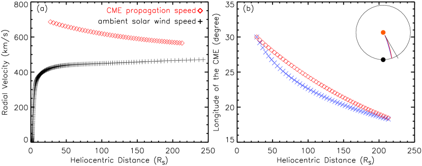
It was shown by Wang et al. (2015) in the statistical study of 72 MCs that the propagation velocity perpendicular to the radial direction is 19 km s-1 on average, and only 8% of the events had a perpendicular velocity larger than 60 km s-1. Thus, the -component propagation velocity in this case is significant enough to indicate an eastward deflection of the MC from the radial direction. By comparing to the radial propagation speed, we may infer that the deflection rate in the ecliptic plane, , is about . Assuming that the CME kept the deflection rate all the way from , where the CME left the FOV of the LASCO/C3 (Fig.1g), to 1 AU, the deflection angle can be calculated by the equation 17 in Wang et al. (2015), i.e., . The change of the CME’s propagation direction estimated by this method is shown as the blue crosses in Figure 5b. Such an eastward deflection made the path of the Earth cutting through the CME closer to the CME center, and therefore enhanced the geoeffectiveness of the initially west-oriented CME.
It is interesting to think about the cause of the possible eastward deflection of the CME. First, the fast stream following the CME clearly modified the MC structure by, e.g., increasing the strength of the magnetic field in the rear portion of the MC, but we think that it probably is not the major cause of the eastward deflection. This CME is a structure embedded in a co-rotating interaction region (CIR) characterized by the fast stream behind the CME and the slow stream ahead of it. One may imagine that the overtaking fast stream would push the CME toward the west. The solar image, e.g., Fig. 2a, also suggests that the CME should be deflected toward the west because of the presence of the large CH on the south-east of it. However, it is probably not the case as implied by the in-situ data and the VFR model results. Thus, we think that the CME’s trajectory was actually controlled by the slow stream ahead of it. The velocity difference between the CME and the preceding slow stream is about 10 times (roughly estimated by eyes from the in-situ data) of that between the CME and the following fast stream. Based on the DIPS picture (Wang et al., 2004, 2014), such velocity differences may lead to a more significant pile-up of solar wind plasma and magnetic field ahead or on the west of the CME than that behind or on the east of it, and therefore cause an eastward deflection.
Now we use the DIPS model to infer the CME trajectory with the constraints of the solar and in-situ observations. To run the DIPS model, we need the CME propagation speed and the ambient solar wind speed, both of which are the functions of the heliocentric distance. As in Wang et al. (2014), the ambient solar wind speed is obtained from the 3-dimensional (3D) MHD simulation (Feng et al., 2003, 2005; Shen et al., 2009, 2011b) for Carrington Rotation 2161 which covered the period from February 29 to March 27. We choose the simulated solar wind speed along the latitude of and within the longitude of –, along which the CME propagated, to generate the averaged solar wind speed (the black plus signs in Fig.5a).
The CME propagation speed is derived by the drag-based model (DBM, Vršnak et al., 2010, 2013), starting at the distance of with the initial speed of the CME leading edge km s-1. The simulated solar wind speed mentioned above is adopted. We adjust the drag coefficient to match the DBM model output, the arrival time of the MC and the speed, with the in-situ observations at 1 AU. After several trials, the best value of is found to be about km-1, with which the modeled MC arrival time is 13:32 UT and the speed of the MC leading edge is 622 km s-1 at 1 AU, close to the observed arrival time 13:05 UT and measured speed of about 600 km s-1. It should be noted that the speed of the CME leading edge consists of two components: the propagation speed and the expansion speed. The VFR model has suggested that the expansion speed is approximated to be one tenth of the CME radial propagation speed. The ratio of the expansion speed to the radial propagation speed will hold as long as the CME self-similarly evolved with a constant angular width. By deducting the expansion speed from the speed of the CME leading edge, we obtain the CME propagation speed as the function of the distance (see red diamonds in Fig.5a).
The red diamonds in Figure 5b show the trajectory of the CME derived from the DIPS model. It is suggested that, from to 1 AU, the CME was deflected by about toward the east, in agreement with the deflection angle, , estimated by the VFR model based on the in-situ observations. It is difficult to evaluate the error of the predicted deflection angle. The direct error comes from the uncertainties in both the CME and solar wind speeds. By considering an uncertainty of in them, the predicted deflection angle of this CME is about . However, since DIPS is a kinematic model, the error may also come from other unknown factors which are not included in the model. In the previous study by Wang et al. (2014), the deflection angle of the slow CME originating on 2008 September 12 is predicted as , which is much smaller than the expected value, , derived from the observations. Thus the same problem is also applicable to the fast CME investigated here.
5 Summary
Here, we study the fast CME originating on 2015 March 15, which caused the largest geomagnetic storm so far in solar cycle 24. With the aid of forward modeling, the kinematic properties of the CME in the corona are obtained based on the solar imaging data. Within 30 the CME propagated west of the Sun-Earth line along the longitude of about and the latitude of about . The propagation speed is about 817 km s-1. Its angular width is wide enough to make its east flank overlap the Sun-Earth line. On the other hand, the in-situ data at 1 AU suggests the flank of a MC arriving at the Earth. Two different models are applied to the MC to infer the configuration of the MC. It is found that the handedness is consistent but the orientation of the flux rope is quite different between the models. As suggested by Riley et al. (2004), such a large deviation in the orientation is probably due to the spacecraft being too far away from the MC’s axis. Currently, it is still difficult to evaluate the reliability of the model results.
Due to the lack of the STEREO observations, the propagation of the 2015 March CME in the heliosphere is unclear. We then try to recover the interplanetary evolution process of the CME from the information at the two ends: near the Sun and at 1 AU. The VFR model results based on the in-situ data suggest that the CME experienced a significant eastward deflection with the ratio of of about , implying a -deflection toward the Earth. The detailed trajectory of the CME between the two ends are further reconstructed by using the numerical simulation (for background solar wind), DBM model (for the CME propagation speed) and DIPS model (for the CME trajectory) under the constraints of the CME’s kinematics obtained from the solar and in-situ observations. The reconstructed trajectory is bent toward the Earth, quite consistent with the deflection implied by the VFR model. This eastward deflection pushed the center of the initially west-oriented CME closer to the Earth and probably contributed to the unexpected strong geoeffectiveness of the CME. However, the lack of interplanetary observations causes that the above inference for this case cannot be fully validated though it sounds reasonable, and the origin of this strong geomagnetic storm is still somewhat mysterious.
Some models applied in this study can be run and tested online. One can go to http://space.ustc.edu.cn/dreams/ for the DIPS model and the VFR model, and to http://oh.geof.unizg.hr/DBM/dbm.php for the DBM model.
Acknowledgements.
We acknowledge the use of the data from SOHO, SDO and Wind spacecraft and the images from Kanzelhoehe Observatory. SOHO is a mission of international cooperation between ESA and NASA, and SDO is a mission of NASA’s Living With a Star Program. We also acknowledge the discussion of the event with T. Berger, N. Gopalswamy, P. Hess, Y. Liu, K. Marubashi, C. Moestl, T. Rollett, M. Temmer, C.-C. Wu and S. Yashiro, under the ISEST program. We thank the anonymous referees for their constructive comments. This work is supported by grants from NSFC (41131065, 41421063), CAS (Key Research Program KZZD-EW-01 and 100-Talent Program), and the fundamental research funds for the central universities. Y.W. is also supported by NSFC 41574165, C.S. by NSFC 41274173, F.S. and Z.Y. by NSFC 41474152 and MOST 973 key project 2012CB825601, and R.L. by NSFC 41222031. B.V. and T.Z. acknowledge the financial support by Croatian Science Foundation under the project 6212 “Solar and Stellar Variability”.References
- Bothmer and Schwenn (1998) Bothmer, V., and R. Schwenn, The structure and origin of magnetic clouds in the solar wind, Ann. Geophys., 16, 1, 1998.
- Brueckner et al. (1995) Brueckner, G. E., et al., The large angle spectroscopic coronagraph (LASCO), Sol. Phys., 162, 357–402, 1995.
- Burlaga (1988) Burlaga, L. F., Magnetic clouds and force-free field with constant alpha, J. Geophys. Res., 93, 7217, 1988.
- Cane and Richardson (2003) Cane, H. V., and I. G. Richardson, Interplanetary coronal mass ejections in the near-earth solar wind during 1996–2002, J. Geophys. Res., 108(A4), 1156, doi:10.1029/2002JA009,817, 2003.
- Cane et al. (2000) Cane, H. V., I. G. Richardson, and O. C. St. Cyr, Coronal mass ejections, interplanetary ejecta and geomagnetic storms, Geophys. Res. Lett., 27, 3591–3594, 2000.
- Cid et al. (2002) Cid, C., M. A. Hidalgo, T. Nieves-Chinchilla, J. Sequeiros, and A. F. Viñas, Plasma and magnetic field inside magnetic clouds: a global study, Sol. Phys., 207, 187–198, 2002.
- Cremades and Bothmer (2004) Cremades, H., and V. Bothmer, On the three-dimensional configuration of coronal mass ejections, Astron. & Astrophys., 422, 307–322, 2004.
- Cremades et al. (2006) Cremades, H., V. Bothmer, and D. Tripathi, Properties of structured coronal mass ejections in solar cycle 23, Adv. in Space Res., 38, 461–465, 2006.
- Feng et al. (2003) Feng, X., S. T. Wu, F. Wei, and Q. Fan, A class of TVD type combined numerical scheme for MHD equations with a survey about numerical methods in solar wind simulations, Space Sci. Rev., 107, 43–53, 2003.
- Feng et al. (2005) Feng, X., C. Xiang, D. Zhong, and Q. Fan, A comparative study on 3-d solar wind structure observed by Ulysses and MHD simulation, Chinese Sci. Bull., 50, 672–678, 2005.
- Goldstein (1983) Goldstein, H., On the field configuration in magnetic clouds, in Sol. Wind Five, p. 731, NASA Conf. Publ. 2280, Washington D. C., 1983.
- Good and Forsyth (2016) Good, S., and R. Forsyth, Interplanetary coronal mass ejections observed by MESSENGER and Venus Express, Sol. Phys., 291, 239–263, 2016.
- Gopalswamy et al. (2003) Gopalswamy, N., M. Shimojo, W. Lu, S. Yashiro, K. Shibasaki, and R. A. Howard, Prominence eruptions and coronal mass ejection: A statistical study using microwave observations, Astrophys. J., 586, 562–578, 2003.
- Gopalswamy et al. (2009) Gopalswamy, N., P. Mäkelä, H. Xie, S. Akiyama, and S. Yashiro, CME interactions with coronal holes and their interplanetary consequences, J. Geophys. Res., 114, A00A22, 2009.
- Gui et al. (2011) Gui, B., C. Shen, Y. Wang, P. Ye, J. Liu, S. Wang, and X. Zhao, Quantitative analysis of cme deflections in the corona, Sol. Phys., 271, 111–139, 2011.
- Hidalgo and Nieves-Chinchilla (2012) Hidalgo, M. A., and T. Nieves-Chinchilla, A global magnetic topology model for magnetic clouds. i., Astrophys. J., 748, 109(7pp), 2012.
- Hidalgo et al. (2002) Hidalgo, M. A., T. Nieves-Chinchilla, and C. Cid, Elliptical cross-section model for the magnetic topology of magnetic clouds, Geophys. Res. Lett., 29, 1637, 2002.
- Hoeksema et al. (2014) Hoeksema, J. T., et al., The helioseismic and magnetic imager (HMI) vector magnetic field pipeline: Overview and performance, Sol. Phys., 289, 3483–3530, 2014.
- Howard and Harrison (2013) Howard, T. A., and R. A. Harrison, Stealth coronal mass ejections: A perspective, Sol. Phys., 285, 269–280, 2013.
- Hu and Sonnerup (2002) Hu, Q., and B. U. O. Sonnerup, Reconstruction of magnetic clouds in the solar wind: Orientations and configurations, J. Geophys. Res., 107, 1142, 2002.
- Hu et al. (2004) Hu, Q., C. W. Smith, N. F. Ness, and R. M. Skoug, Multiple flux rope magnetic ejecta in the solar wind, J. Geophys. Res., 109(A3), A03,102, 2004.
- Isavnin et al. (2013) Isavnin, A., A. Vourlidas, and E. K. J. Kilpua, Three-dimensional evolution of erupted flux ropes from the Sun (2–20 r) to 1 AU, Sol. Phys., 284, 203–215, 2013.
- Isavnin et al. (2014) Isavnin, A., A. Vourlidas, and E. K. J. Kilpua, Three-dimensional evolution of flux-rope CMEs and its relation to the local orientation of the heliospheric current sheet, Sol. Phys., 289, 2141–2156, 2014.
- Janvier et al. (2013) Janvier, M., P. Démoulin, and S. Dasso, Global axis shape of magnetic clouds deduced from the distribution of their local axis orientation, Astron. & Astrophys., 556, A50, 2013.
- Kaiser et al. (2008) Kaiser, M. L., T. A. Kucera, J. M. Davila, O. C. St. Cyr, M. Guhathakurta, and E. Christian, The stereo mission: An introduction, Space Sci. Rev., 136, 5–16, 2008.
- Kataoka et al. (2015) Kataoka, R., D. Shiota, E. Kilpua, and K. Keika, Pileup accident hypothesis of magnetic storm on 17 March 2015, Geophys. Res. Lett., 42, 5155–5161, 2015.
- Kay and Opher (2015) Kay, C., and M. Opher, The heliocentric distance where the deflections and rotations of solar coronal mass ejections occur, Astrophys. J. Lett., 811, L36(6pp), 2015.
- Kay et al. (2013) Kay, C., M. Opher, and R. M. Evans, Forecasting a coronal mass ejection’s altered trajectory: ForeCAT, Astrophys. J., 775, 5(17pp), 2013.
- Kilpua et al. (2009) Kilpua, E. K. J., J. Pomoell, A. Vourlidas, R. Vainio, J. Luhmann, Y. Li, P. Schroeder, A. B. Galvin, and K. Simunac, STEREO observations of interplanetary coronal mass ejections and prominence deflection during solar minimum period, Ann. Geophys., 27, 4491–4503, 2009.
- Lemen et al. (2012) Lemen, J. R., et al., The atmospheric imaging assembly (AIA) on the solar dynamics observatory (SDO), Sol. Phys., 275, 17–40, 2012.
- Lepping et al. (1990) Lepping, R. P., J. A. Jones, and L. F. Burlaga, Magnetic field structure of interplanetary magnetic clouds at 1 AU, J. Geophys. Res., 95, 11,957–11,965, 1990.
- Lepping et al. (1995) Lepping, R. P., et al., The Wind magnetic field investigation, Space Sci. Rev., 71, 207–229, 1995.
- Lin et al. (1995) Lin, R. P., et al., A three-dimensional plasma and energetic particle investigation for the Wind spacecraft, Space Sci. Rev., 71, 125–153, 1995.
- Liu et al. (2015) Liu, Y. D., H. Hu, R. Wang, Z. Yang, B. Zhu, Y. A. Liu, J. G. Luhmann, and J. D. Richardson, Plasma and magnetic field characteristics of solar coronal mass ejections in relation to geomangetic strom intensity and variability, Astrophys. J. Lett., 809, L34(6pp), 2015.
- Lopez and Freeman (1986) Lopez, R. E., and J. W. Freeman, Solar wind proton temperature-velocity relationship, J. Geophys. Res., 91, 1701, 1986.
- Lugaz et al. (2010) Lugaz, N., J. N. Hernandez-Charpak, I. I. Roussev, C. J. Davis, A. Vourlidas, and J. A. Davies, Determining the azimuthal properties of coronal mass ejections from multi-spacecraft remote-sensing observations with STEREO SECCHI, Astrophys. J., 715, 493–499, 2010.
- MacQueen et al. (1986) MacQueen, R. M., A. J. Hundhausen, and C. W. Conover, The propagation of coronal mass ejection transients, J. Geophys. Res., 91, 31–38, 1986.
- Marubashi (1986) Marubashi, K., Structure of the interplanetary magnetic clouds and their solar origins, Adv. in Space Res., 6, 335–338, 1986.
- Marubashi and Lepping (2007) Marubashi, K., and R. P. Lepping, Long-duration magnetic clouds: a comparison of analyses using torus- and cylinder-shaped flux rope models, Ann. Geophys., 25, 2453–2477, 2007.
- Möstl et al. (2015) Möstl, C., et al., Strong coronal channelling and interplanetary evolution of a solar storm up to Earth and Mars, Nature Commun., 6, 7135, 2015.
- Mulligan and Russell (2001) Mulligan, T., and C. T. Russell, Multispacecraft modeling of the flux rope structure of interplanetary coronal mass ejections: Cylindrically symmetric versus nonsymmetric topologies, J. Geophys. Res., 106(A6), 10,581–10,596, 2001.
- Mulligan et al. (1998) Mulligan, T., C. T. Russell, and J. G. Luhmann, Solar cycle evolution of the structure of magnetic clouds in the inner heliosphere, Geophys. Res. Lett., 25, 2959–2962, 1998.
- Ogilvie et al. (1995) Ogilvie, K. W., et al., SWE, a comprehensive plasma instrument for the Wind spacecraft, Space Sci. Rev., 71, 55–77, 1995.
- Riley et al. (2004) Riley, P., et al., Fitting flux ropes to a global MHD solution: a comparison of techniques, J. Atmos. Solar-Terres. Phys., 66, 1321–1331, 2004.
- Robbrecht et al. (2009) Robbrecht, E., S. Patsourakos, and A. Vourlidas, No trace left behind: STEREO observation of a coronal mass ejection without low coronal signatures, Astrophys. J., 701, 283–291, 2009.
- Romashets and Vandas (2003) Romashets, E. P., and M. Vandas, Force-free field inside a toroidal magnetic cloud, Geophys. Res. Lett., 30, 2065, 2003.
- Rust and Kumar (1996) Rust, K., and A. Kumar, Evidence for helical kinked magnetic flux ropes in solar eruptions, Astrophys. J. Lett., 464, L199–L202, 1996.
- Shen et al. (2011a) Shen, C., Y. Wang, B. Gui, P. Ye, and S. Wang, Kinematic evolution of a slow CME in near solar space viewed by STEREO-B in October 8, 2007, Sol. Phys., 269, 389–400, 2011a.
- Shen et al. (2009) Shen, F., X. Feng, and W. B. Song, An asynchronous and parallel time-marching method: application to the three-dimensional MHD simulation of the solar wind, Science in china Series E: Technological Sciences, 52, 2895–2902, 2009.
- Shen et al. (2011b) Shen, F., X. S. Feng, Y. Wang, S. T. Wu, W. B. Song, J. P. Guo, and Y. F. Zhou, Three-dimensional MHD simulation of two coronal mass ejections’ propagation and interaction using a successive magnetized plasma blobs model, J. Geophys. Res., 116, A09,103, 2011b.
- Thernisien (2011) Thernisien, A., Implementation of the graduated cylindrical shell model for the three-dimensional reconstruction of coronal mass ejections, Astrophys. J. Suppl. Ser., 194, 33, 2011.
- Thernisien et al. (2009) Thernisien, A., A. Vourlidas, and R. Howard, Forward modeling of coronal mass ejections using STEREO/SECCHI data, Sol. Phys., 256, 111–130, 2009.
- Vandas and Romashets (2003) Vandas, M., and E. P. Romashets, A force-free field with constant alpha in an oblate cylinder: A generalization of the lundquist solution, Astron. & Astrophys., 398, 801–807, 2003.
- Vršnak et al. (2010) Vršnak, B., T. Žic, T. V. Falkenberg, C. Möstl, S. Vennerstrom, and D. Vrbanec, The role of aerodynamic drag in propagation of interplanetary coronal mass ejections, Astron. & Astrophys., 512, A43, 2010.
- Vršnak et al. (2013) Vršnak, B., et al., Propagation of interplanetary coronal mass ejections: The drag-based model, Sol. Phys., 285, 295–315, 2013.
- Wang et al. (2002) Wang, Y., P. Z. Ye, S. Wang, G. P. Zhou, and J. X. Wang, A statistical study on the geoeffectiveness of earth-directed coronal mass ejections from March 1997 to December 2000, J. Geophys. Res., 107(A11), 1340, doi:10.1029/2002JA009,244, 2002.
- Wang et al. (2004) Wang, Y., C. Shen, P. Ye, and S. Wang, Deflection of coronal mass ejection in the interplanetary medium, Sol. Phys., 222, 329–343, 2004.
- Wang et al. (2006) Wang, Y., X. Xue, C. Shen, P. Ye, S. Wang, and J. Zhang, Impact of the major coronal mass ejections on geo-space during September 7 – 13, 2005, Astrophys. J., 646, 625–633, 2006.
- Wang et al. (2011) Wang, Y., C. Chen, B. Gui, C. Shen, P. Ye, and S. Wang, Statistical study of coronal mass ejection source locations: Understanding cmes viewed in coronagraphs, J. Geophys. Res., 116, A04,104, doi:10.1029/2010JA016,101, 2011.
- Wang et al. (2014) Wang, Y., B. Wang, C. Shen, F. Shen, and N. Lugaz, Deflected propagation of a coronal mass ejection from the corona to interplanetary space, J. Geophys. Res., 119, 5117–5132, 2014.
- Wang et al. (2015) Wang, Y., Z. Zhou, C. Shen, R. Liu, and S. Wang, Investigating plasma motion of magnetic clouds at 1 AU through a velocity-modified cylindrical force-free flux rope model, J. Geophys. Res., 120, 1543–1565, 2015.
- Webb et al. (2001) Webb, D. F., N. U. Crooker, S. P. Plunkett, and O. C. St. Cyr, The solar sources of geoeffective structures, in Space Weather, edited by S. Paul, J. S. Howard, and L. S. George, Geophys. Monogr. Ser. 125, pp. 123–142, AGU, 2001.
- Wood et al. (2016) Wood, B. E., J. L. Lean, S. E. McDonald, and Y.-M. Wang, Comparative ionospheric impacts and solar origins of nine strong geomagnetic storms in 2010-2015, J. Geophys. Res., accepted, doi:10.1002/2015JA021,953, 2016.
- Yermolaev et al. (2005) Yermolaev, Y. I., M. Yermolaev, G. Zastenker, L. Zelenyi, A. Petrukovich, and J.-A. Sauvaud, Statistical studies of geomagnetic storm dependencies on solar and interplanetary events: a review, Planet. Space Sci., 53, 189–196, 2005.
- Zhang et al. (2007) Zhang, J., et al., Solar and interplanetary sources of major geomagnetic storms (Dst -100 nT) during 1996-2005, J. Geophys. Res., 112, A10,102, 2007.
- Zhao and Webb (2003) Zhao, X. P., and D. F. Webb, Source regions and storm effectiveness of frontside full halo coronal mass ejections, J. Geophys. Res., 108(A6), 1234, 2003.
- Zuccarello et al. (2012) Zuccarello, F. P., A. Bemporad, C. Jacobs, M. Mierla, S. Poedts, and F. Zuccarello, The role of streamers in the deflection of coronal mass ejections: Comparison between STEREO three-dimensional reconstructions and numerical simulations, Astrophys. J., 744, 66(14pp), 2012.