Robustness of Distributed Averaging Control in Power Systems: Time Delays & Dynamic Communication Topology

Abstract

Distributed averaging-based integral (DAI) controllers are becoming increasingly popular in power system applications. The literature has thus far primarily focused on disturbance rejection, steady-state optimality and adaption to complex physical system models without considering uncertainties on the cyber and communication layer nor their effect on robustness and performance. In this paper, we derive sufficient delay-dependent conditions for robust stability of a secondary-frequency-DAI-controlled power system with respect to heterogeneous communication delays, link failures and packet losses. Our analysis takes into account both constant as well as fast-varying delays, and it is based on a common strictly decreasing Lyapunov-Krasovskii functional. The conditions illustrate an inherent trade-off between robustness and performance of DAI controllers. The effectiveness and tightness of our stability certificates are illustrated via a numerical example based on Kundur’s four-machine-two-area test system.

1 Introduction

1.1 Motivation

Power systems worldwide are currently experiencing drastic changes and challenges. One of the main driving factors for this development is the increasing penetration of distributed and volatile renewable generation interfaced to the network with power electronics accompanied by a reduction in synchronous generation. This results in power systems being operated under more and more stressed conditions [1]. In order to successfully cope with these changes, the control and operation paradigms of today’s power systems have to be adjusted to the new conditions. The increasing complexity in terms of network dynamics and number of active network elements renders centralized and inflexible approaches inappropriate creating a clear need for robust and distributed solutions with plug-and-play capabilities [2]. The latter approaches require a combination of advanced control techniques with adequate communication technologies.

Multi-agent systems (MAS) represent a promising framework to address these challenges [3]. A popular distributed control strategy for MAS are distributed averaging-based integral (DAI) algorithms, also known as consensus filters [4, 5] that rely on averaging of integral actions through a communication network. The distributed character of this type of protocol has the advantage that no central computation unit is needed and the individual agents, i.e., generation units, only have to exchange information with their neighbors [6].

One of the most relevant control applications in power systems is frequency control which is typically divided into three hierarchical layers: primary, secondary and tertiary control [7]. In the present paper, we focus on secondary control which is tasked with the regulation of the frequency to a nominal value in an economically efficient way and subject to maintaining the net area power balance. The literature on secondary DAI frequency controllers addressing these tasks is reviewed in the following.

1.2 Literature Review on DAI Frequency Control

DAI algorithms have been proposed previously to address the objectives of secondary frequency control in bulk power systems [8, 9, 10, 11] and also in microgrids (i.e., small-footprint power systems on the low and medium voltage level) [12, 6, 13]. They have been extended to achieve asymptotically optimal injections [14, 15], and have also been adapted to increasingly complex physical system models [16, 17]. The closed-loop DAI-controlled power system is a cyber-physical system whose stability and performance crucially relies on nearest-neighbor communication. Despite all recent advances, communication-based controllers (in power systems) are subject to considerable uncertainties such as message delays, message losses, and link failures [18, 2] that can severely reduce the performance – or even affect the stability – of the overall cyber-physical system. Such cyber-physical phenomena and uncertainties have not been considered thus far in DAI-controlled power systems.

For microgrids, the effect of communication delays on secondary controllers has been considered in [19] for the case of a centralized PI controller, in [20] for a centralized PI controller with a Smith predictor as well as a model predictive controller and in [21] for a DAI-controlled microgrid with fixed communication topology. In all three papers, a small-signal (i.e., linearization-based) analysis of a model with constant delays is performed.

In [22, 23] distributed control schemes for microgrids are proposed, and conditions for stability under time-varying delays as well as a dynamic communication topology are derived. However, both approaches are based on the pinning-based controllers requiring a master-slave architecture. Compared to the DAI controller in the present paper, this introduces an additional uncertainty as the leader may fail (see also Remark 1 in [23]). In addition, the analysis in [22, 23] is restricted to the distributed control scheme on the cyber layer and neglects the physical dynamics. Moreover, the control in [22] is limited to power sharing strategies, and secondary frequency regulation is not considered.

The delay robustness of alternative distributed secondary control strategies (based on primal-dual decomposition approaches) has been investigated for constant delays and a linearized power system model in [24, 25].

1.3 Contributions

The present paper addresses both the cyber and the physical aspects of DAI frequency control by deriving conditions for robust stability of nonlinear DAI-controlled power systems under communication uncertainties. With regards to delays, we consider constant as well as fast-varying delays. The latter are a common phenomenon in sampled data networked control systems, due to digital control [26, 27, 28] and as the network access and transmission delays depend on the actual network conditions, e.g., in terms of congestion and channel quality [29]. In addition to delays, in practical applications the topology of the communication network can be time-varying due to message losses and link failures [30, 5, 31]. This can be modeled by a switching communication network [30, 5]. Thus, the explicit consideration of communication uncertainties leads to a switched nonlinear power system model with (time-varying) delays the stability of which is investigated in this paper.

More precisely, our main contributions are as follows. First, we derive a strict Lyapunov function for a nominal DAI-controlled power system model without communication uncertainties, which may also be of independent interest. Second, we extend this strict Lyapunov function to a common Lyapunov-Krasovskii functional (LKF) to provide sufficient delay-dependent conditions for robust stability of a DAI-controlled power system with dynamic communication topology as well as heterogeneous constant and fast-varying delays. Our stability conditions can be verified without exact knowledge of the operating state and reflect a fundamental trade-off between robustness and performance of DAI control. Third and finally, we illustrate the effectiveness of the derived approach on a numerical benchmark example, namely Kundur’s four-machine-two-area test system [7, Example 12.6].

The remainder of the paper is structured as follows. In Section 2 we recall some preliminaries on algebraic graph theory and introduce the power system model employed for the analysis. The DAI control is motivated and introduced in Section 3, where we also derive a suitable error system. A strict Lyapunov function for the closed-loop DAI-controlled power system is derived in Section 4. Based on this Lyapunov function, we then construct a common LKF for DAI-controlled power systems with constant and fast-varying delays in Section 5. A numerical example is provided in Section 6. The paper is concluded with a brief summary and outlook on future work in Section 7.

Notation. We define the sets ${}_{\geq 0}:=\{x\in\real|x\geq 0\}$, ${}_{>0}:=\{x\in\real|x>0\}$ and ${}_{<0}:=\{x\in\real|x<0\}.$ For a set $\mathcal{V},$ $|\mathcal{V}|$ denotes its cardinality and $[\mathcal{V}]^{k}$ denotes the set of all subsets of $\mathcal{V}$ that contain $k$ elements. Let $x=\text{col}(x_{i})\in{}^{n}$ denote a vector with entries $x_{i}$ for $i\in\{1,\dots,n\}$, $\mathbbold{0}_{n}$ the zero vector, $\mathbbold{1}_{n}$ the vector with all entries equal to one, $I_{n}$ the $n\times n$ identity matrix, $\mathbbold{0}_{n\times n}$ the $n\times n$ matrix with all entries equal to zero and $\mbox{diag}(a_{i})$ an $n\times n$ diagonal matrix with diagonal entries $a_{i}\in\real.$ Likewise, $A=\text{blkdiag}(A_{i})$ denotes a block-diagonal matrix with block-diagonal matrix entries $A_{i}.$ For $A\in{}^{n\times n},$ $A>0$ means that $A$ is symmetric positive definite. The elements below the diagonal of a symmetric matrix are denoted by $\ast.$ We denote by $W[-h,0],$ $h\in{}_{>0},$ the Banach space of absolutely continuous functions $\phi:[-h,0]\to{}^{n},$ $h\in{}_{>0},$ with $\dot{\phi}\in L_{2}(-h,0)^{n}$ and with the norm $\|\phi\|_{W}=\max_{\theta\in[a,b]}|\phi(\theta)|+\left({\int_{-h}^{0}{\dot{\phi}}^{2}d\theta}\right)^{0.5}$. Also, $\nabla f$ denotes the gradient of a function $f:{}^{n}\to\real.$

2 Preliminaries

2.1 Algebraic Graph Theory

An undirected graph of order $n$ is a tuple $\mathcal{G}=(\mathcal{N},\mathcal{E}),$ where $\mathcal{N}=\{1,\ldots,n\}$ is the set of nodes and $\mathcal{E}\subseteq[\mathcal{N}]^{2},$ $\mathcal{E}=\{e_{1},\ldots,e_{m}\},$ is the set of undirected edges, i.e., the elements of $\mathcal{E}$ are subsets of $\mathcal{N}$ that contain two elements. In the context of the present work, each node in the graph represents a generation unit. The adjacency matrix $\mathcal{A}\in{}^{|\mathcal{N}|\times|\mathcal{N}|}$ has entries $a_{ik}=a_{ki}=1$ if an edge between $i$ and $k$ exists and $a_{ik}=0$ otherwise. The degree of a node $i$ is defined as $d_{i}=\sum_{k=1}^{|\mathcal{N}|}a_{ik}.$ The Laplacian matrix of an undirected graph is given by $\mathcal{L}=\mathcal{D}-\mathcal{A},$ where $\mathcal{D}=\mbox{diag}(d_{i})\in{}^{|\mathcal{N}|\times|\mathcal{N}|}.$ An ordered sequence of nodes such that any pair of consecutive nodes in the sequence is connected by an edge is called a path. A graph $\mathcal{G}$ is called connected if for all pairs $\{i,k\}\in[\mathcal{N}]^{2}$ there exists a path from $i$ to $k$. The Laplacian matrix $\mathcal{L}$ of an undirected graph is positive semidefinite with a simple zero eigenvalue if and only if the graph is connected. The corresponding right eigenvector to this simple zero eigenvalue is $\mathbbold{1}_{n}$, i.e., $\mathcal{L}\mathbbold{1}_{n}=\mathbbold{0}_{n}$ [32]. We refer the reader to [33, 32] for further information on graph theory.

2.2 Power Network Model

We consider a Kron-reduced [34, 7] power system model composed of $n\geq 1$ nodes. The set of network nodes is denoted by $\mathcal{N}=\{1,\ldots,n\}.$ Following standard practice, we make the following assumptions: the line admittances are purely inductive and the voltage amplitudes $V_{i}\in{}_{>0}$ at all nodes $i\in\mathcal{N}$ are constant [7]. To each node $i\in\mathcal{N},$ we associate a phase angle $\theta_{i}:{}_{\geq 0}\to\real$ and denote its time derivative by $\omega_{i}=\dot{\theta}_{i},$ which represents the electrical frequency at the $i$-th node. Under the made assumptions, two nodes $i$ and $k$ are connected via a nonzero susceptance $B_{ik}\in{}_{<0}.$ If there is no line between $i$ and $k,$ then $B_{ik}=0.$ We denote by $\mathcal{N}_{i}=\{k\in\mathcal{N}\,|\,B_{ik}\neq 0\}$ the set of neighboring nodes of the $i$-th node. Furthermore, we assume that for all $\{i,k\}\in[\mathcal{N}]^{2}$ there exists an ordered sequence of nodes from $i$ to $k$ such that any pair of consecutive nodes in the sequence is connected by a power line represented by an admittance, i.e., the electrical network is connected.

We consider a heterogeneous generation pool consisting of rotational synchronous generators (SGs) and inverter-interfaced units. The former are the standard equipment in conventional power networks and mostly used to connect fossil-fueled generation to the network. Compared to this, most renewable and storage units are connected via inverters, i.e., power electronics equipment, to the grid. We assume that all inverter-interfaced units are fitted with droop control and power measurement filters, see [35, 36]. This implies that their dynamics admit a mathematically equivalent representation to SGs [36, 37]. Hence, the dynamics of the generation unit at the $i$-th node, $i\in\mathcal{N},$ considered in this paper is given by

$$\begin{split}\dot{\theta}_{i}&=\omega_{i},\\ M_{i}\dot{\omega}_{i}&=-D_{i}(\omega_{i}-\omega^{d})+P_{i}^{d}-G_{ii}V_{i}^{2}+u_{i}-P_{i},\end{split}$$ (1)

where $D_{i}\in{}_{>0}$ is the damping or (inverse) droop coefficient, $\omega^{d}\in{}_{>0}$ is the nominal frequency, $P_{i}^{d}\in\real$ is the active power setpoint and $G_{ii}V_{i}^{2},$ $G_{ii}\in{}_{\geq 0},$ represents the (constant active power) load at the $i$-th node. Furthermore, $u_{i}:{}_{\geq 0}\to\real$ is a control input and $M_{i}\in{}_{>0}$ is the (virtual) inertia coefficient, which in case of an inverter-interfaced unit is given by $M_{i}=\tau_{P_{i}}D_{i},$ where $\tau_{P_{i}}\in{}_{>0}$ is the low-pass filter time constant of the power measurement filter, see [39, 36]. Following standard practice in power systems, all parameters are assumed to be given in per unit [7]. The active power flow $P_{i}:{}^{n}\to\real$ is given by

$$P_{i}=\sum\nolimits_{k\in\mathcal{N}_{i}}|B_{ik}|V_{i}V_{k}\sin(\theta_{ik}),$$

where we have introduced the short-hand $\theta_{ik}=\theta_{i}-\theta_{k}.$ For a detailed modeling of the system components, the reader is referred to [40, 36].

To derive a compact model representation of the power system, it is convenient to introduce the matrices

$$\begin{split}&D=\mbox{diag}(D_{i})\in{}^{n\times n},\,M=\mbox{diag}(M_{i})\in{}^{n\times n},\\ \end{split}$$

and the vectors

$$\begin{split}&\theta=\text{col}(\theta_{i})\in{}^{n},\,\omega=\text{col}(\omega_{i})\in{}^{n},\\ &P^{\text{net}}=\text{col}(P_{i}^{d}-G_{ii}V_{i}^{2})\in{}^{n},\,u=\text{col}(u_{i})\in{}^{n}.\end{split}$$

Also, we introduce the potential function $U:{}^{n}\to\real,$

$$U(\theta)=-\sum\nolimits_{\{i,k\}\in[\mathcal{N}]^{2}}|B_{ik}|V_{i}V_{k}\cos(\theta_{ik}).$$

Then, the dynamics (1), $\forall i\in\mathcal{N},$ can be compactly written as

$$\begin{split}\dot{\theta}&=\omega,\\ M\dot{\omega}&=-D(\omega-\mathbbold{1}_{n}\omega^{d})+P^{\text{net}}+u-\nabla_{\theta}U(\theta).\end{split}$$ (2)

Observe that due to symmetry of the power flows $P_{i},$

$$\mathbbold{1}_{n}^{\top}\nabla_{\theta}U(\theta)=0.$$ (3)

3 Nominal DAI-Controlled Power System Model with Fixed Communication Topology and no Delays

In this section, the employed secondary control scheme is motivated and introduced. Subsequently, we derive the considered resulting nominal closed-loop system, i.e., without delays and switched topology. For this model, we construct a suitable error system and a strict Lyapunov function in Section 4, both of which are instrumental to establish the robust stability results under communication uncertainties in Section 5.

3.1 Secondary Frequency Control: Objectives and Distributed Averaging Integral (DAI) Control

The whole power system is designed to work at, or at least very close to, the nominal network frequency $\omega^{d}$ [7]. However, by inspection of a synchronized solution (i.e., a solution with constant uniform frequencies $\omega^{*}=\omega^{s}\mathbbold{1}_{n},$ constant control input $u^{*}$ and constant phase angle differences $\theta^{*}_{ik}$) of the system (2), we have that

$$0=\mathbbold{1}_{n}^{\top}M\dot{\omega}=\mathbbold{1}_{n}^{\top}(-D\mathbbold{1}_{n}(\omega^{s}-\omega^{d})+P^{\text{net}}+u^{*}-\nabla_{\theta}U(\theta^{*})),$$

which with (3) implies that

$$\omega^{s}=\omega^{d}+\frac{\mathbbold{1}_{n}^{\top}(P^{\text{net}}+u^{*})}{\mathbbold{1}_{n}^{\top}D\mathbbold{1}_{n}}.$$ (4)

Note that the loads $G_{ii}V_{i}^{2}$ contained in $P^{\text{net}}$ are usually unknown. Hence, in general $\mathbbold{1}_{n}^{\top}P^{\text{net}}\neq 0$ and, thus, $\omega^{s}\neq\omega^{d},$ unless the additional control signal $u^{*}$ accounts for the power imbalance. Control schemes which yield such $u$ and, consequently, ensure $\omega^{s}=\omega^{d}$ are termed secondary frequency controllers.

Building upon [12, 15, 10], we consider the following secondary frequency control scheme for the system (2)

$$\begin{split}u&=-p,\\ \dot{p}&=K(\omega-\mathbbold{1}_{n}\omega^{d})-KA\mathcal{L}Ap.\end{split}$$ (5)

We refer to the control (5) as distributed averaging integral (DAI) control law in the sequel. Here, $K\in{}^{n\times n}$ is a diagonal gain matrix with positive diagonal entries, $\mathcal{L}=\mathcal{L}^{\top}\in{}^{n\times n}$ is the Laplacian matrix of the undirected and connected communication graph over which the individual generation units can communicate with each other, and $A$ is a positive definite diagonal matrix with the element $A_{ii}>0$ being a coefficient accounting for the cost of secondary control at node $i$. It has been shown in [12, 15, 10] that the control law (5) is a suitable secondary frequency control scheme for the system (2), i.e., it can achieve $\omega^{s}=\omega^{d}$ despite unknown (constant) loads; see [8, 11] for variations of the control (5) for dynamic load models. In addition to secondary frequency control, the control law (5) can also ensure that the power injections of all generation units satisfy the identical marginal cost requirement in steady-state, i.e.,

$$A_{ii}u_{i}^{*}=A_{kk}u_{k}^{*}\mbox{ for all }i\in\mathcal{N},\,k\in\mathcal{N}\,,$$ (6)

where $A_{ii}$ and $A_{kk}$ are the respective diagonal entries of the matrix $A.$

The nominal closed-loop system resulting from combining (2) with (5) is given by

$$\begin{split}\dot{\theta}&=\omega,\\ M\dot{\omega}&=-D(\omega-\omega^{d}\mathbbold{1}_{n})+P^{\text{net}}-\nabla_{\theta}U(\theta)-p,\\ \dot{p}&=K(\omega-\mathbbold{1}_{n}\omega^{d})-KA\mathcal{L}Ap.\end{split}$$ (7)

To formalize our main objective, it is convenient to introduce the notion below.

Definition (Synchronized motion).

The system (7) admits a synchronized motion if it has a solution for all $t\geq 0$ of the form

$$\theta^{*}(t)=\theta_{0}^{*}+\omega^{*}t,\quad\omega^{*}=\omega^{s}\mathbbold{1}_{n},\quad p^{*}\in{}^{n},$$

where $\omega^{s}\in\real$ and $\theta_{0}^{*}\in{}^{n}$ such that

$$|\theta_{0,i}^{*}-\theta_{0,k}^{*}|<\frac{\pi}{2}\quad\forall i\in\mathcal{N},\;\forall k\in\mathcal{N}_{i}.$$

Note that [10, Lemma 4.2] implies that the system (7) has at most one synchronized motion $\text{col}(\theta^{*},\omega^{*},p^{*})$ (modulo $2\pi$). That motion also satisfies the identical marginal cost requirement (6) and is characterized by

$$p^{*}=\alpha A^{-1}\mathbbold{1}_{n},\quad\alpha=\frac{\mathbbold{1}_{n}^{\top}P^{\text{net}}}{\mathbbold{1}_{n}^{\top}A^{-1}\mathbbold{1}_{n}}$$ (8)

and, hence, $\omega^{s}=\omega^{d},$ see (4) with $u^{*}=-p^{*}.$

3.2 A Useful Coordinate Transformation

We introduce a coordinate transformation that is fundamental to establish our robust stability results. Recall that $\mathbbold{1}_{n}^{\top}\mathcal{L}=0.$ This results in an invariant subspace of the $p$-variables, which makes the construction of a strict Lyapunov function for the system (7) difficult. Therefore, we seek to eliminate this invariant subspace through an appropriate coordinate transformation. To this end and inspired by [30, 31, 41], we introduce the variables $\bar{p}\in{}^{(n-1)}$ and $\zeta\in\real$ via the transformation

$$\begin{split}\begin{bmatrix}\bar{p}\\ \zeta\end{bmatrix}&=\mathcal{W}^{\top}K^{-\frac{1}{2}}p,\quad\mathcal{W}=\begin{bmatrix}W&\frac{1}{\sqrt{\mu}}K^{-\frac{1}{2}}A^{-1}\mathbbold{1}_{n}\end{bmatrix},\,\end{split}$$ (9)

where $\mu=\|K^{-\frac{1}{2}}A^{-1}\mathbbold{1}_{n}\|_{2}^{2}$ and $W\in{}^{n\times(n-1)}$ has orthonormal columns that are all orthogonal to $K^{-\frac{1}{2}}A^{-1}\mathbbold{1}_{n}$, i.e., $W^{\top}K^{-\frac{1}{2}}A^{-1}\mathbbold{1}_{n}=\mathbbold{0}_{(n-1)}$. Hence, the transformation matrix $\mathcal{W}\in{}^{n\times n}$ is orthogonal, i.e.,

$$\mathcal{W}\mathcal{W}^{\top}\!=\!WW^{\top}+\frac{1}{\mu}K^{-\frac{1}{2}}A^{-1}\mathbbold{1}_{n}\mathbbold{1}_{n}^{\top}K^{-\frac{1}{2}}A^{-1}\!=\!I_{n}.$$ (10)

Accordingly, $\bar{p}$ is a projection of $p$ on the subspace orthogonal to $K^{-\frac{1}{2}}A^{-1}\mathbbold{1}_{n}$ scaled by $K^{-\frac{1}{2}}.$ Furthermore,

$$\zeta=\frac{1}{\sqrt{\mu}}\mathbbold{1}_{n}^{\top}K^{-1}A^{-1}p$$ (11)

can be interpreted as the scaled average secondary control injections of the network. Indeed, from (7) together with the fact that $\mathbbold{1}_{n}^{\top}\mathcal{L}=0,$ we have that

$$\dot{\zeta}=\frac{1}{\sqrt{\mu}}\mathbbold{1}_{n}^{\top}K^{-1}A^{-1}\dot{p}=\frac{1}{\sqrt{\mu}}\mathbbold{1}_{n}^{\top}A^{-1}(\omega-\mathbbold{1}_{n}\omega^{d}),$$

which by integrating with respect to time and recalling (11) yields

$$\begin{split}\zeta&=\frac{1}{\sqrt{\mu}}\mathbbold{1}_{n}^{\top}A^{-1}(\theta-\theta_{0}-\mathbbold{1}_{n}\omega^{d}t+K^{-1}p_{0})\\ &=\frac{1}{\sqrt{\mu}}\mathbbold{1}_{n}^{\top}A^{-1}(\theta-\mathbbold{1}_{n}\omega^{d}t)+\bar{\zeta}_{0},\end{split}$$ (12)

where

$$\bar{\zeta}_{0}=\sqrt{\mu}^{-1}\mathbbold{1}_{n}^{\top}A^{-1}(K^{-1}p_{0}-\theta_{0}).$$ (13)

As a consequence, the coordinate $\zeta$ can be expressed by means of $\theta$ and the parameter $\bar{\zeta}_{0}.$ Hence,

$$\begin{split}p&=K^{\frac{1}{2}}\left(W\bar{p}+\frac{1}{\sqrt{\mu}}K^{-\frac{1}{2}}A^{-1}\mathbbold{1}_{n}\zeta\right)\\ &=K^{\frac{1}{2}}\left(W\bar{p}+\frac{1}{\mu}K^{-\frac{1}{2}}A^{-1}\mathbbold{1}_{n}(\mathbbold{1}_{n}^{\top}A^{-1}(\theta-\mathbbold{1}_{n}\omega^{d}t)+\bar{\zeta}_{0})\right)\,.\end{split}$$ (14)

Accordingly, we define the matrix

$$\bar{\mathcal{L}}=W^{\top}K^{\frac{1}{2}}A\mathcal{L}AK^{\frac{1}{2}}W\in{}^{(n-1)\times(n-1)},$$

that corresponds to the communication Laplacian matrix $\mathcal{L}$ after scaling and projection. Note that $\mathcal{L}$ is connected by assumption, and thus $\bar{\mathcal{L}}$ is positive definite.

In the reduced coordinates, the dynamics (7) become

$$\begin{split}\dot{\theta}&=\omega,\\ M\dot{\omega}&=-D(\omega-\omega^{d}\mathbbold{1}_{n})\!+\!P^{\text{net}}\!-\!\nabla_{\theta}U(\theta)\\ &-\!K^{\frac{1}{2}}\!\left(\!W\bar{p}+\!\frac{1}{\mu}K^{-\frac{1}{2}}A^{-1}\mathbbold{1}_{n}(\mathbbold{1}_{n}^{\top}A^{-1}(\theta\!-\!\mathbbold{1}_{n}\omega^{d}t)+\bar{\zeta}_{0})\!\right)\!,\\ \dot{\bar{p}}&=W^{\top}K^{-\frac{1}{2}}\dot{p}\\ &=W^{\top}K^{\frac{1}{2}}(\omega-\mathbbold{1}_{n}\omega^{d})-\bar{\mathcal{L}}\bar{p},\end{split}$$ (15)

where we have used (14) and the fact that $\mathcal{L}\mathbbold{1}_{n}=\mathbbold{0}_{n}.$ Note that the transformation (9) removes the invariant subspace $\text{span}(\mathbbold{1}_{n})$ of a synchronized motion of (7) in the $\theta$-variables and shifts it to the invariant subspace $\text{span}(K^{-\frac{1}{2}}A^{-1})$, where it is factored out in the orthogonal reduced-order $\bar{p}$-variables.

3.3 Error States

For the subsequent analysis, we make the following standard assumption [37, 10].

Assumption (Existence of synchronized motion).

The closed-loop system (15) possesses a synchronized motion. $\square$

With initial time $t_{0}=0,$ as well as

$$\bar{p}^{*}=W^{\top}K^{-\frac{1}{2}}p^{*},$$

see (9), we introduce the error coordinates

$$\begin{split}\tilde{\omega}&=\omega-\mathbbold{1}_{n}\omega^{d},\quad\tilde{p}=\bar{p}-\bar{p}^{*},\\ \tilde{\theta}&=\theta-\theta^{*}=\theta_{0}-\theta_{0}^{*}+\int_{0}^{t}\tilde{\omega}(s)ds,\\ x&=\text{col}\left(\tilde{\theta},\,\tilde{\omega},\,\tilde{p}\right).\end{split}$$

Then the dynamics (15) become

$$\begin{split}\dot{\tilde{\theta}}=&{\tilde{\omega}},\\ M\dot{\tilde{\omega}}=&-D\tilde{\omega}-\nabla_{\tilde{\theta}}U(\tilde{\theta}+\theta^{*})+\nabla_{\tilde{\theta}}U(\theta^{*})\\ &-\!K^{\frac{1}{2}}W\tilde{p}-\frac{1}{\mu}A^{-1}\mathbbold{1}_{n}\mathbbold{1}_{n}^{\top}A^{-1}\tilde{\theta},\\ \dot{\tilde{p}}=&W^{\top}K^{\frac{1}{2}}\tilde{\omega}-\bar{\mathcal{L}}\tilde{p}\end{split}$$ (16)

and $x^{*}=\mathbbold{0}_{(3n-1)}$ is an equilibrium point of (16). Furthermore, in error coordinates the potential function $U:{}^{n}\to\real$ reads

$$U(\tilde{\theta}+\theta^{*})=-\sum\nolimits_{\{i,k\}\in[\mathcal{N}]^{2}}|B_{ik}|V_{i}V_{k}\cos(\tilde{\theta}_{ik}+\theta^{*}_{ik})$$

with

$$\nabla_{\tilde{\theta}}U(\tilde{\theta}+\theta^{*})=\frac{\partial U(\tilde{\theta}+\theta^{*})}{\partial\tilde{\theta}},\;\nabla_{\tilde{\theta}}U(\theta^{*})=\frac{\partial U(\tilde{\theta}+\theta^{*})}{\partial\tilde{\theta}}\big{|}_{\tilde{\theta}=\mathbbold{0}_{n}}.$$

Recall from Section 3.1 that any synchronized motion of the system (7) satisfies $\omega^{s}=\omega^{d}$ and that $p^{*}$ is uniquely given by (8). Thus, for a fixed value of $\bar{\zeta}_{0}$ it follows from (13) together with (14) that asymptotic stability of $x^{*}$ implies convergence of the solutions $\text{col}(\theta,\omega,p)$ of the original system (7) with initial conditions that satisfy

$$\bar{\zeta}_{0}=\sqrt{\mu}^{-1}\mathbbold{1}_{n}^{\top}A^{-1}(K^{-1}p_{0}-\theta_{0})$$

to a synchronized motion $\text{col}(\theta^{*},\omega^{*},p^{*}),$ the initial angles $\theta_{0}^{*}$ of which satisfy

$$\bar{\zeta}_{0}=\sqrt{\mu}^{-1}\mathbbold{1}_{n}^{\top}A^{-1}(K^{-1}p^{*}-\theta^{*}_{0}).$$

As this holds true for any value of $\bar{\zeta}_{0}$ and the dynamics (16) are independent of $\bar{\zeta}_{0},$ asymptotic stability of $x^{*}$ implies convergence of all solutions of the original system (7) to a synchronized motion.

4 Stability Analysis of the Nominal Closed-Loop System with a Strict Lyapunov Function

To pave the path for the analysis in Section 5, we start by investigating stability of an equilibrium $x^{*}$ of the nominal (without delays and with constant communication topology) closed-loop system (16).

The proposition below provides a stability proof for an equilibrium of the system (16) by employing the following strict Lyapunov function candidate

$$\begin{split}V=&U(\tilde{\theta}+\theta^{*})-\tilde{\theta}^{\top}\nabla_{\tilde{\theta}}U(\theta^{*})+\frac{1}{2}\tilde{\omega}^{\top}M\tilde{\omega}\\ &+\frac{1}{2\mu}(\mathbbold{1}_{n}^{\top}A^{-1}\tilde{\theta})^{2}+\frac{1}{2}\tilde{p}^{\top}\tilde{p}\\ &+\epsilon\tilde{\omega}^{\top}AM(\nabla_{\tilde{\theta}}U(\tilde{\theta}+\theta^{*})-\nabla_{\tilde{\theta}}U(\theta^{*})),\end{split}$$ (17)

where $\epsilon>0$ is a positive real and sufficiently small parameter. The Lyapunov function (17) is based on the classic kinetic and potential energy terms $\omega^{\top}M\omega$ and $U(\theta)$ [42] written in error coordinates, a Bregman construction to center the Lyapunov function as in [11, 8], a Chetaev-type cross term between the (incremental) potential and kinetic energies [43], and a quadratic term for the secondary control inputs (also in error coordinates). We have the following result.

Proposition (Stability of the nominal system).

Consider the system (16) with Assumption 3.3. The function $V$ in (17) is a strict Lyapunov function for the system (16). Furthermore, $x^{*}=\mathbbold{0}_{(3n-1)}$ is locally asymptotically stable. $\square$

We first show that the function $V$ in (17) is locally positive definite. It is easily verified that

$$\nabla V\big{|}_{x^{*}}=\mathbbold{0}_{(3n-1)}.$$

Moreover, the Hessian of $V$ evaluated at $x^{*}$ is given by

$$\nabla V^{2}\big{|}_{x^{*}}=\begin{bmatrix}\nabla_{\tilde{\theta}}^{2}U|_{x^{*}}+\frac{1}{\mu}A^{-1}\mathbbold{1}_{n}\mathbbold{1}_{n}^{\top}A^{-1}&\frac{\epsilon}{2}E_{12}&\mathbbold{0}\\ \ast&M&\mathbbold{0}\\ \ast&\ast&I_{(n-1)}\end{bmatrix},$$

where

$$E_{12}=AM\nabla_{\tilde{\theta}}^{2}U|_{x^{*}}+\nabla_{\tilde{\theta}}^{2}U|_{x^{*}}MA$$

and $\mathbbold{0}$ denotes a zero matrix of appropriate dimension. Under the standing assumptions, $\nabla_{\tilde{\theta}}^{2}U|_{x^{*}}$ is a Laplacian matrix of an undirected connected graph. Hence, $\nabla_{\tilde{\theta}}^{2}U|_{x^{*}}$ is positive semidefinite with $\ker(\nabla_{\tilde{\theta}}^{2}U|_{x^{*}})=\text{span}(\mathbbold{1}_{n}).$ Furthermore, $A^{-1}\mathbbold{1}_{n}\mathbbold{1}_{n}^{\top}A^{-1}$ is positive semidefinite and $\ker(A^{-1}\mathbbold{1}_{n}\mathbbold{1}_{n}^{\top}A^{-1})\cap\ker(\nabla_{\tilde{\theta}}^{2}U|_{x^{*}})=\mathbbold{0}_{n}.$ In addition, $M$ is a diagonal matrix with positive diagonal entries. Thus, all block-diagonal entries of $\nabla V^{2}\big{|}_{x^{*}}$ are positive definite. This implies that there is a sufficiently small $\epsilon^{*}>0$ such that for all $\epsilon\in{]0,\epsilon^{*}]}$ we have that $\nabla V^{2}\big{|}_{x^{*}}>0.$ We choose such $\epsilon.$ Therefore, $x^{*}$ is a strict minimum of $V.$

The time derivative of $V$ along solutions of (16) is given by

$$\begin{split}\!\!\!\dot{V}\!&\!=-\xi^{\top}\!\!\begin{bmatrix}\epsilon A&0.5\epsilon AD&0.5\epsilon AK^{\frac{1}{2}}W\!\\ \ast&D\!-\!0.5\epsilon E_{22}&\mathbbold{0}_{n\times(n-1)}\\ \ast&\ast&\bar{\mathcal{L}}\end{bmatrix}\!\xi,\!\!\end{split}$$ (18)

where we have used the property that

$$(\nabla_{\tilde{\theta}}U(\tilde{\theta}+\theta^{*})-\nabla_{\tilde{\theta}}U(\theta^{*}))^{\top}\mathbbold{1}_{n}=0$$

and defined the shorthand

$$E_{22}=(AM\nabla_{\tilde{\theta}}^{2}U(\tilde{\theta}+\theta^{*})+\nabla_{\tilde{\theta}}^{2}U(\tilde{\theta}+\theta^{*})AM),$$ (19)

as well as

$$\xi=\text{col}\left(\nabla_{\tilde{\theta}}U(\tilde{\theta}+\theta^{*})-\nabla_{\tilde{\theta}}U(\theta^{*}),\,\tilde{\omega},\,\tilde{p}\right).$$

Note that the matrix $E_{22}$ only depends on the cosines of the angles $\tilde{\theta}.$ Hence, there is a positive real constant $\gamma,$ such that $E_{22}\leq\gamma I_{n}$ for all $\tilde{\theta}\in{}^{n}.$ Furthermore, $A,$ $D$ and $\bar{\mathcal{L}}$ are positive definite matrices. Thus, Lemma 1 in Appendix A implies that there is a sufficiently small $\epsilon^{**}\in{(0,\epsilon^{*}]}$ such that for any $\epsilon\in{(0,\epsilon^{**}]}$ the matrix on the right-hand side of (18) is positive definite and, thus, $\dot{V}<0$ for all $\xi\neq\mathbbold{0}_{(3n-1)}.$ Consequently, by choosing such $\epsilon,$ $V$ is a strict Lyapunov function for the system (16) and, by Lyapunov’s theorem [44], $x^{*}$ is asymptotically stable, completing the proof. $\square$

5 Stability of the Closed-Loop System with Dynamic Communication Topology and Delays

This section is dedicated to the analysis of cyber-physical aspects in the form of communication uncertainties on the performance of the DAI-controlled power system model (16).

5.1 Modeling and Problem Formulation

Recall from Section 1 that the most relevant practical communication uncertainties in the context of DAI control are message delays, message losses and link failures. We follow the approaches in [30, 5, 31, 27, 28] to model these phenomena.

Thus, link failures and packet losses are modeled by a dynamic communication network with switched communication topology $\mathcal{G}_{\sigma(t)},$ where $\sigma:{}_{\geq 0}\to\mathcal{M}$ is a switching signal and $\mathcal{M}=\{1,2,\ldots,\nu\},$ $\nu\in{}_{>0},$ is an index set. The finite set of all possible network topologies amongst $|\mathcal{N}|=n$ nodes is denoted by $\Gamma=\{\mathcal{G}_{1},\mathcal{G}_{2},\ldots\mathcal{G}_{\nu}\}.$ The Laplacian matrix corresponding to the index $\ell=\sigma(t)\in\mathcal{M}$ is denoted by $\mathcal{L}_{\ell}=\mathcal{L}_{\ell}^{\top}=\mathcal{L}(\mathcal{G}_{\ell})\in{}^{n\times n}.$ We employ the following standard assumption on $\mathcal{G}_{\sigma(t)}$ [30, 5].

Assumption .

(Uniformly connected communication topologies) The communication topology $\mathcal{G}_{\sigma(t)}$ is undirected and connected for all $t\in{}_{\geq 0}.$ $\square$

With regards to communication delays, we suppose that a message sent by generation unit $k\in\mathcal{N}$ to the generation unit $i\in\mathcal{N}$ over the communication channel (i.e., edge) $\{i,k\}$ is affected by a fast-varying delay $\tau_{ik}:{}_{\geq 0}\to[0,h],$ $h\in{}_{\geq 0}$, where the qualifier ”fast-varying” means that there are no restrictions imposed on the existence, continuity, or boundedness of $\dot{\tau}_{ik}(t)$ [27, 28]. The resulting control error $e_{ik}$ is then computed as

$$e_{ik}(t)=A_{ii}p_{i}(t-\tau_{ik}(t))-A_{kk}p_{k}(t-\tau_{ik}(t)),$$

i.e., the protocol is only executed after the message from node $k$ arrives at node $i.$ Note that we allow for asymmetric delays, i.e., $\tau_{ik}(t)\neq\tau_{ki}(t).$ Furthermore, as standard in sampled-data networked control systems [27, 28], the delay $\tau_{ik}(t)$ may be piecewise-continuous in $t$. Also, we assume that the switches in topology don’t modify the delays between two connected nodes.

In order to write the resulting closed-loop system compactly, we introduce the matrices $T_{\ell,m}\in{}^{n\times n},$ $m=1,\ldots,2|\mathcal{E}_{\ell}|,$ where $|\mathcal{E}_{\ell}|$ is the number of edges of the undirected graph with index $\ell=\sigma(t)\in\mathcal{M}$ of the dynamic communication network of the DAI control (5), $m$ denotes the information flow from node $i$ to $k$ over the edge $\{i,k\}$ with delay $\tau_{m}=\tau_{ik}$ and all elements of $T_{\ell,m}$ are zero besides the entries

$$t_{\ell,m,ii}=1,\quad t_{\ell,m,ik}=-1.$$ (20)

As we allow for $\tau_{ik}\neq\tau_{ki},$ we require $2|\mathcal{E}_{\ell}|$ matrices $T_{\ell,m}$ in order to distinguish between the delayed information flow from $k$ to $i$ (with delay $\tau_{ik}$) and that from $k$ to $i$ (with delay $\tau_{ki}$). Note that by summing over all $T_{\ell,m}$ we recover the full Laplacian matrix of the communication network corresponding to the topology index $\ell=\sigma(t)\in\mathcal{M}$, i.e.,

$$\mathcal{L}_{\ell}=\sum_{m=1}^{2|\mathcal{E}_{\ell}|}T_{\ell,m}.$$

With the above considerations, the closed-loop system (7) becomes the switched nonlinear delay-differential system

$$\begin{split}\dot{\theta}&=\omega,\\ M\dot{\omega}&=-D(\omega-\omega^{d}\mathbbold{1}_{n})+P^{\text{net}}-\nabla_{\theta}U(\theta)-p,\\ \dot{p}&=K(\omega-\mathbbold{1}_{n}\omega^{d})-KA\left(\sum_{m=1}^{2|\mathcal{E}_{\ell}|}T_{\ell,m}Ap(t-\tau_{m})\right),\end{split}$$ (21)

where $\tau_{m}(t)\in[0,h_{m}],$ $m=1,\ldots,2|\mathcal{E}_{\ell}|$ are fast-varying delays and $T_{\ell,m}$ corresponds to the $m$-th delayed (directed) channel of the $\ell$-th communication topology corresponding to the topology index $\ell=\sigma(t)\in\mathcal{M}$ of the dynamic communication network of the DAI control (5).

We are interested in the following problem.

Problem .

(Conditions for robust stability) Consider the system (21). Given $h_{m}\in{}_{\geq 0},$ $m=1,\ldots,2\bar{\mathcal{E}},$ $\bar{\mathcal{E}}=max_{\ell\in\mathcal{M}}{|\mathcal{E}_{\ell}|},$ derive conditions under which the solutions of the system (21) converge asymptotically to a synchronized motion. $\square$

As in the nominal scenario, we make the assumption below.

Assumption (Existence of synchronized motion).

The closed-loop system (21) possesses a synchronized motion. $\square$

From (14) it follows that for any $m=1,\ldots,2\bar{\mathcal{E}},$

$$p(t-\tau_{m})=\!K^{\frac{1}{2}}\!\left(\!W\bar{p}(t-\tau_{m})+\frac{1}{\sqrt{\mu}}K^{-\frac{1}{2}}A^{-1}\mathbbold{1}_{n}\zeta(t-\tau_{m})\!\right),$$

which together with the fact that by construction, see (20), $T_{\ell,m}\mathbbold{1}_{n}=\mathbbold{0}_{n}$ implies that

$$T_{\ell,m}Ap(t-\tau_{m})=T_{\ell,m}AK^{\frac{1}{2}}W\bar{p}(t-\tau_{m}).$$

Hence, with Assumption 5.1 and by following the steps in Section 3, we represent the system (21) in reduced-order error coordinates as, cf., (16),

$$\begin{split}\dot{\tilde{\theta}}=&{\tilde{\omega}},\\ M\dot{\tilde{\omega}}=&-D\tilde{\omega}-\nabla_{\tilde{\theta}}U(\tilde{\theta}+\theta^{*})+\nabla_{\tilde{\theta}}U(\theta^{*})\\ &-\!K^{\frac{1}{2}}W\tilde{p}-\frac{1}{\mu}A^{-1}\mathbbold{1}_{n}\mathbbold{1}_{n}^{\top}A^{-1}\tilde{\theta},\\ \dot{\tilde{p}}=&W^{\top}K^{\frac{1}{2}}\tilde{\omega}-\sum_{m=1}^{2|\mathcal{E}|}\mathcal{T}_{\ell,m}\tilde{p}(t-\tau_{m}),\end{split}$$ (22)

where we defined, analogous to $\bar{\mathcal{L}}$,

$$\mathcal{T}_{\ell,m}=W^{\top}K^{\frac{1}{2}}AT_{\ell,m}AK^{\frac{1}{2}}W\in{}^{(n-1)\times(n-1)},$$ (23)

which satisfies

$$\sum_{m=1}^{2|\mathcal{E}_{\ell}|}\mathcal{T}_{\ell,m}=W^{\top}K^{\frac{1}{2}}A\mathcal{L}_{\ell}AK^{\frac{1}{2}}W=:\bar{\mathcal{L}}_{\ell}.$$ (24)

Note that, by assumption, the graph associated to $\mathcal{L}_{\ell}$ is connected and thus $\bar{\mathcal{L}_{\ell}}$ is positive definite for any $\ell\in\mathcal{M}$.

By construction, the system (22) has an equilibrium point $z^{*}=\text{col}(\tilde{\theta},\tilde{\omega},\tilde{p})=\mathbbold{0}_{(3n-1)}.$ Furthermore, by the same arguments as in Section 3.1, asymptotic stability of $z^{*}$ implies convergence of the solutions of the system (21) to a synchronized motion. As a consequence of this fact, we provide a solution to Problem 5.1 by studying stability of $z^{*}.$

5.2 Stability of the Closed-Loop System with Dynamic Communication Topology and Delays

We analyze stability of equilibria of the system (22) with dynamic communication topology and time delays. The result is formulated for fast-varying piecewise-continuous bounded delays $\tau_{m}(t)\in[0,h_{m}]$ with $h_{m}\in{}_{\geq 0},$ $m=1,\ldots,2\bar{\mathcal{E}}.$ For the case of constant delays, stability can be verified via the same conditions.

To streamline our main result, we recall from Section 3 that the matrix $A$ can be used to achieve the objective of identical marginal costs. As a consequence, the choice of $A$ influences the corresponding equilibria of the system (22), see (8). But the equilibria are independent of the integral control gain matrix $K.$ Hence, we may chose $K$ as a free tuning parameter to ensure stability of the closed-loop system (22). The proof of the proposition below is given in Appendix B.

Proposition (Robust stability).

Consider the system (22) with Assumptions 5.1 and 5.1. Fix $A$ and $D$ as well as some $h_{m}\in{}_{\geq 0},$ $m=1,\ldots,2\bar{\mathcal{E}}.$ Select $K$ such that for all $\mathcal{T}_{\ell,m}$ and $\bar{\mathcal{L}}_{\ell}$ defined in (23), respectively (24), $\ell=1,\ldots,|\mathcal{M}|,$ there exist matrices $S_{m}>0\in{}^{(n-1)\times(n-1)},$ $R_{m}>0\in{}^{(n-1)\times(n-1)}$ and $S_{12,m}\in{}^{(n-1)\times(n-1)}$ satisfying

$$\Psi=\begin{bmatrix}\Psi_{11}&\Psi_{12}&\mathbbold{0}&\Psi_{14}\\ \ast&\Psi_{22}&\Psi_{23}&\Psi_{24}\\ \ast&\ast&R+S&S_{12}+S\\ \ast&\ast&\ast&R+S+\bar{\Psi}_{44}\end{bmatrix}>0,$$ (25)

where

$$\begin{split}R&=\text{blockdiag}(R_{m}),\;S=\text{blockdiag}(S_{m}),\\ S_{12}&=\text{blockdiag}(S_{12,m}),\;\bar{R}=\sum_{j=1}^{2\bar{\mathcal{E}}}h_{j}^{2}R_{j},\\ \Psi_{11}&=D-K^{\frac{1}{2}}W\bar{R}W^{\top}K^{\frac{1}{2}},\;\Psi_{22}=\bar{\mathcal{L}}_{\ell}-\bar{\mathcal{L}}_{\ell}\bar{R}\bar{\mathcal{L}}_{\ell},\\ \bar{\Psi}_{44}&=\text{blockdiag}\left(-\mathcal{T}_{\ell,m}^{\top}\bar{R}\mathcal{T}_{\ell,m}\right),\\ \Psi_{12}&=K^{\frac{1}{2}}W\bar{R}\bar{\mathcal{L}}_{\ell},\;\Psi_{23}=-\begin{bmatrix}S_{1}&\ldots&S_{2\bar{\mathcal{E}}}\end{bmatrix},\\ \Psi_{14}&=\begin{bmatrix}\bar{\Psi}_{14,1}&\ldots&\bar{\Psi}_{14,{2\bar{\mathcal{E}}}}\end{bmatrix},\;\Psi_{24}=\begin{bmatrix}\bar{\Psi}_{24,1}&\ldots&\bar{\Psi}_{24,{2\bar{\mathcal{E}}}}\end{bmatrix},\\ \bar{\Psi}_{14,m}&=-K^{\frac{1}{2}}W\bar{R}\mathcal{T}_{\ell,m},\\ \bar{\Psi}_{24,m}&=\bar{\mathcal{L}}_{\ell}\bar{R}\mathcal{T}_{\ell,m}-S_{m}-0.5\mathcal{T}_{\ell,m},\end{split}$$ (26)

$\mathbbold{0}$ denotes a zero matrix of appropriate dimensions and

$$\begin{bmatrix}R&S_{12}\\ \ast&R\end{bmatrix}\geq 0.$$ (27)

Then the equilibrium $z^{*}=\mathbbold{0}_{(3n-1)}$ is locally uniformly asymptotically stable for all fast-varying delays $\tau_{m}(t)\in[0,h_{m}].$ $\square$

The stability certificate (25), (27) is based on a LKF derived from the Lyapunov function (17), and it is fairly tight (see Section 6). Note that the evaluation of the certificate (25), (27) and the corresponding controller tuning inherently is centralized and requires complete system information. However, the stability certificate (25), (27) can be also made wieldy for a practical plug-and-play control implementation by trading off controller performance for robust stability. The following corollary makes this idea precise for the case of uniform delays, i.e., $\tau_{m}(t)=\tau(t)\in[0,h],$ $h_{m}=h,$ $h\in{}_{\geq 0},$ $m=1,\ldots,2\bar{\mathcal{E}}.$

Corollary (Performance-robustness-trade-off).

Consider the system (22) with Assumptions 5.1 and 5.1. Fix $A$ and $D$ as well as some $h\in{}_{\geq 0}.$ Suppose that $\tau_{m}(t)=\tau(t)\in[0,h]$ and that (27) is satisfied with strict inequality. Set $K=\kappa\mathcal{K},$ where $\kappa\in{}_{\geq 0}$ and $\mathcal{K}\in{}_{>0}^{n\times n}$ is a diagonal matrix with positive diagonal entries. Then there is $\kappa>0$ sufficiently small, such that the equilibrium $z^{*}=\mathbbold{0}_{(3n-1)}$ is locally uniformly asymptotically stable for all fast-varying delays $\tau(t)\in[0,h].$

With $K=\kappa\mathcal{K},$ we have that

$$\mathcal{T}_{\ell,m}=\kappa\hat{\mathcal{T}}_{\ell,m},\quad\bar{\mathcal{L}}_{\ell}=\kappa\hat{\mathcal{L}}_{\ell}=\kappa\sum_{m=1}^{2\bar{\mathcal{E}}}\hat{\mathcal{T}}_{\ell,m},$$

with $\mathcal{T}_{\ell,m}$ and $\bar{\mathcal{L}}_{\ell}$ defined in (23), respectively (24). Furthermore, we write the free parameter matrix $S$ as $S=\kappa\mathcal{S},$ $\mathcal{S}>0.$ Consequently, the matrices in (26) also become $\kappa$-dependent. Then, for $\tau_{m}(t)=\tau(t)\leq h$ the matrix $\Psi$ in (25) can be written as

$$\Psi=\begin{bmatrix}D&\mathbbold{0}&\mathbbold{0}&\mathbbold{0}\\ \ast&\mathbbold{0}&\mathbbold{0}&\mathbbold{0}\\ \ast&\ast&R&S_{12}\\ \ast&\ast&\ast&R\end{bmatrix}+\kappa\begin{bmatrix}\Phi_{11}&\Phi_{12}&\mathbbold{0}&\Phi_{14}\\ \ast&\Phi_{22}&-\mathcal{S}&\Phi_{24}\\ \ast&\ast&\mathcal{S}&\mathcal{S}\\ \ast&\ast&\ast&\Phi_{44}\end{bmatrix},$$ (28)

where

$$\begin{split}\Phi_{11}&=-h^{2}\mathcal{K}^{\frac{1}{2}}WRW^{\top}\mathcal{K}^{\frac{1}{2}},\,\Phi_{12}=h^{2}\kappa^{\frac{1}{2}}\mathcal{K}^{\frac{1}{2}}WR\hat{\mathcal{L}}_{\ell},\\ \Phi_{22}&=\hat{\mathcal{L}}_{\ell}-h^{2}\kappa\hat{\mathcal{L}}_{\ell}R\hat{\mathcal{L}}_{\ell},\,\Phi_{44}=\mathcal{S}-h^{2}\kappa\bar{\mathcal{L}}_{\ell}R\bar{\mathcal{L}}_{\ell},\\ \Phi_{14}&=-h^{2}\kappa^{\frac{1}{2}}\mathcal{K}^{\frac{1}{2}}WR\hat{\mathcal{L}}_{\ell},\,\Phi_{24}=h^{2}\kappa\hat{\mathcal{L}}_{\ell}R\hat{\mathcal{L}}_{\ell}-\mathcal{S}-0.5\hat{\mathcal{L}}_{\ell}.\end{split}$$ (29)

Note that $\Phi_{22}$ can be written as

$$\hat{\mathcal{L}}_{\ell}\left(\hat{\mathcal{L}}_{\ell}^{-1}-h^{2}\kappa R\right)\hat{\mathcal{L}}_{\ell}.$$ (30)

Hence, by continuity, for any given $\hat{\mathcal{L}}_{\ell}>0$ and $R>0$ we can find a small enough $\kappa,$ such that $\Phi_{22}>0.$ In addition, $D>0$ and (27) is satisfied with strict inequality by assumption. Therefore, the matrix $\Psi$ in (28) is a parameter-dependent composite matrix of the form stated in Lemma 1. Consequently, Lemma 1 implies that for given $h,$ $A,$ $D$ and $\mathcal{L}_{\ell},$ $\ell=1,\ldots,\nu,$ there is always a sufficiently small gain $\kappa$ such that there exist matrices $\mathcal{S},$ $R$ and $S_{12}$ satisfying conditions (25), (27). $\square$

The claim in Corollary 5.2 is in a very similar spirit to the result obtained in [30, 5] for the standard linear consensus protocol with delays. In essence, Corollary 5.2 shows that there is a trade-off between delay-robustness, i.e., feasibility of conditions (25), (27) and a high gain matrix $K$ for the DAI controller (5). Aside from displaying an inherent performance-robustness trade-off, Corollary 5.2 allows us to certify robust stability (for any switched communication topology) based merely on sufficiently small control gains and without evaluating a linear matrix inequality in a centralized fashion.

We remark that it is also possible to obtain a completely decentralized (though in general more conservative) tuning criterion by further bounding the matrices in (28), respectively (25).

Remark .

Conditions (25), (27) are linear matrix inequalities that can be efficiently solved via standard numerical tools, e.g., [45]. Furthermore, instead of checking (25), (27) for all $\bar{\mathcal{L}}_{\ell}$ it also suffices to do so for their convex hull [46]. In addition, checking the convex hull gives a robustness criterion for all unknown topology configurations within the chosen convex hull. Compared to the related results on stability of delayed port-Hamiltonian systems with application to microgrids with delays [47, 48], the conditions (25), (27) are independent of the specific equilibrium point $z^{*}.$ $\square$

Remark .

Note that $\hat{\mathcal{L}}_{\ell}^{-1}\geq{1}/{\lambda_{\max}(\hat{\mathcal{L}}_{\ell})}I_{(n-1)},$ where $\lambda_{\max}(\hat{\mathcal{L}}_{\ell})$ denotes the maximum eigenvalue of the matrix $\hat{\mathcal{L}}_{\ell},$ $\ell=1,\ldots,\nu.$ Hence, (30) shows that the admissible largest gain $\kappa$ in order for $\Phi_{22}$ (defined in (29)) to be positive definite is constrained by the maximum eigenvalue of all matrices $\hat{\mathcal{L}}_{\ell}.$ This fact is confirmed by the numerical experiments in Section 6. Similar observations have also been made numerically for consensus systems [31]. $\square$

6 Numerical Example

We illustrate the effectiveness of the proposed approach on Kundur’s four-machine-two-area test system [7, Example 12.6]. The considered test system is shown in Fig. 1. The employed parameters are as given in [7, Example 12.6] with the only difference that we set the damping constants to $D_{i}=1/(0.05\cdot 2\pi\cdot 60)$ pu (with respect to the machine loading $S_{\text{SG}}=[700,700,719,700]$ MVA). The system base power is $S_{\text{B}}=900$ MVA, the base voltage is $V_{\text{B}}=230$ kV and the base frequency is $\omega_{\text{B}}=1$ rad/s.

For the tests, we consider the four different communication network topologies shown in Fig. 1. Topology $\mathcal{G}_{1}$ is the nominal topology, representing a ring graph. In topology $\mathcal{G}_{2},$ respectively $\mathcal{G}_{3}$ and $\mathcal{G}_{4},$ one of the links is broken. Note that each of the configurations is connected and, hence, the dynamic communication network given by the topologies $\Gamma=\{\mathcal{G}_{1},\mathcal{G}_{2},\mathcal{G}_{3},\mathcal{G}_{4}\}$ satisfies Assumption 5.1. Furthermore, we set $A=\mbox{diag}(S_{\text{SG}}/S_{\text{B}})$ and $K=\kappa\mathcal{K},$ where $\mathcal{K}=0.05A^{-1}$ and $\kappa$ is a free tuning parameter.

We consider an exemplary scenario with fast-varying delays $\tau_{m}\in[0,h_{m}]$s, $h_{m}=2$s, $m=1,\ldots,2\bar{\mathcal{E}}.$ With the chosen parameters, we check conditions (25), (27). The numerical implementation is done in Yalmip [45]. In order to identify the maximum admissible gain $\kappa,$ we select an initial value for $\kappa$ of $\kappa_{\text{init}}=2.0$ and iteratively decrease the value of $\kappa$ until conditions (25), (27) are satisfied. The obtained feasible gain is $\kappa_{\text{feas}}=1.544.$

The simulation results shown in Fig. 2 confirm the fact that the systems’ trajectories converge to a synchronized motion if $\kappa_{\text{feas}}=1.544.$ Following standard practice in sampled-data networked control systems [27, 28], the time-varying delays are implemented as piecewise-continuous signals. For the present simulations, we have used the rate transition and variable time delay blocks in Matlab/Simulink with a sampling time $T_{s}=2$ms to generate the fast-varying delays. During the simulation, the communication topology switches randomly every $0.5$s. Variations in the switching interval did not lead to meaningful changes in the system’s behavior. This shows that the DAI control is very robust to dynamic changes in the communication topology. Furthermore, our experiments confirm the observation in Remark 5.2 and [31] that for a given upper bound on the delay the feasibility of conditions (25), (27) is highly dependent on the largest eigenvalue of the Laplacian matrices.

We verify the conservativeness of the sufficient conditions (25), (27) in simulation. Recall that the conditions are equilibrium-independent. Hence, if feasible they guarantee (local) stability of any equilibrium point satisfying the standard requirement of the equilibrium angle differences being contained in an arc of length $\pi/2,$ cf. Assumption 5.1. Therefore, we consider three different operating conditions: at first, the nominal equilibrium point $z^{*,1}$ reported in [7, Example 12.6] and subsequently two operating points $z^{*,2}$ and $z^{*,3}$ under more stressed conditions, i.e., with some angle differences being closer to the ends of the $\pi/2$-arc. The angles for all three scenarios are given in Table 1.

For the nominal operating point $z^{*,1}$ the maximum feasible gain obtained for fast-varying delays with $h_{m}=2$s via simulation experiments is $\kappa_{\text{feas,sim}}=6.330.$ For higher values of $\kappa,$ the system exhibits limit cycling behavior. The value of $\kappa_{\text{feas,sim}}=6.330$ is about $4.1$ times larger than the value of $\kappa_{\text{feas}}=1.544$ obtained via Proposition 5.2. In the case of $z^{*,2}$ and with the same delays the maximum feasible gain identified via simulation is $\kappa_{\text{feas,sim}}=2.856,$ which is about $1.85$ times larger as the value of $\kappa_{\text{feas}}=1.544$ obtained from conditions (25), (27). The maximum feasible gain is further reduced in the last operating scenario with equilibrium $z^{*,3},$ where we obtain $\kappa_{\text{feas,sim}}=1.698.$ This value is only $1.1$ times larger than the value of $\kappa_{\text{feas}}=1.544$ obtained from conditions (25), (27). We observe a very similar behavior in the case of constant delays. This shows that - for the investigated scenarios - our (equilibrium-independent) conditions are fairly conservative at equilibria corresponding to less stressed operating conditions, while they are almost exact under highly stressed operating conditions.

Table 1: Values of phase angles at considered equilibria $z^{*,1}$ to $z^{*,3}.$

$\theta^{*,1}$ [rad]	$[0.224,0.117,-0.076,-0.189]\cdot\pi/2$
$\theta^{*,2}$ [rad]	$[0.3,-0.4,-0.5,0.4]\cdot 3\pi/8$
$\theta^{*,3}$ [rad]	$[0.3,-0.4,-0.5,0.4]\cdot\pi/2$

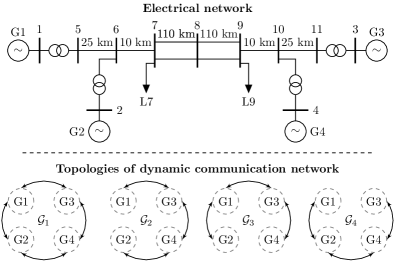
Figure 1: Kundur’s two-area-four-machine test system taken from [7, Example 12.6] and below the four different topologies of the switched communication network.

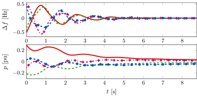
Figure 2: Simulation example for $\kappa=1.544,$ $h_{m}=2$s, $m=1,\ldots,4$ and arbitrary initial conditions in a neighborhood of $z^{*,1}$. The lines correspond to the following units: G1 ’–’, G2 ’- -’, G3 ’+-’ and G4 ’* -’.

7 Conclusions

We have considered the problem of robust stability of a DAI-controlled power system with respect to cyber-physical uncertainties in the form of constant and fast-varying communication delays as well as link failures and packet losses. The phenomena of link failures and packet losses lead to a time-varying communication topology with arbitrary switching. For this setup, we have derived sufficient delay-dependent stability conditions by constructing a suitable common LKF. The stability conditions can be verified without knowledge of the operating point and reflect a performance and robustness trade-off, which is in a very similar manner to that of the standard linear consensus protocol with delays investigated in [30, 5].

In addition, the approach has been applied to Kundur’s two-area-four-machine test system. The numerical experiments show that our sufficient equilibrium-independent conditions are very tight for stressed operating points, i.e., with (some) stationary angle differences close to $\pm\pi/2,$ while they are more conservative for less stressed operating points.

In future research we will seek to relax some of the modeling assumptions made in the paper, e.g., on constant voltage amplitudes, constant load models, and investigate further applications of DAI and related distributed control methods to power systems and microgrids. Another interesting, yet technically challenging, open question is to weaken the connectivity assumption imposed on the DAI communication network, e.g., by using the notion of joint connectivity [49].

Appendix

Appendix A A Matrix Regularization Lemma

Lemma 1 (Matrix regularization).

Consider the two symmetric real block matrices

$$A=\begin{bmatrix}\mathbbold{0}_{p\times p}&\mathbbold{0}_{p\times q}\\ \ast&A_{22}\end{bmatrix}\quad\text{ and }\quad B=\begin{bmatrix}B_{11}&B_{12}\\ \ast&B_{22}\end{bmatrix},$$

with $A_{22}\in{}^{q\times q},B_{11}\in{}^{p\times p},\,B_{22}\in{}^{q\times q},\,B_{12}\in{}^{p\times q}.$ Suppose that $A_{22}$ and $B_{11}$ are positive definite. Then there exists a (sufficiently small) positive real $\epsilon$ such that the composite matrix $C_{\epsilon}=A+\epsilon B$ is positive definite.

The composite matrix reads as

$$C_{\epsilon}=\begin{bmatrix}\epsilon B_{11}&\epsilon B_{12}\\ \ast&A_{22}+\epsilon B_{22}\end{bmatrix}\,.$$

As $B_{11}$ is positive definite by assumption, $\epsilon B_{11}>0$ for any $\epsilon>0.$ Furthermore, by applying the Schur complement to $C_{\epsilon}$ we obtain

$$A_{22}+\epsilon\left(B_{22}-B_{12}^{\top}B_{11}^{-1}B_{12}\right),$$

which, as $A_{22}>0$ by assumption, is positive definite for small enough $\epsilon$. The latter together with $\epsilon B_{11}>0$ implies that $C_{\epsilon}>0$ for small enough $\epsilon$, completing the proof. $\square$

Appendix B Proof of Proposition 5.2

We give the proof of Proposition 5.2. The proof is inspired by [31, 27, 47, 48] and established by constructing a common LKF for the system (22). Consider the LKF with $m=1,\ldots,2\bar{\mathcal{E}},$

$$\begin{split}\mathcal{V}=&V+\sum_{m=1}^{2\bar{\mathcal{E}}}\mathcal{V}_{1,m}+\sum_{m=1}^{2\bar{\mathcal{E}}}\mathcal{V}_{2,m},\\ \mathcal{V}_{1,m}&=\int_{t-h_{m}}^{t}\tilde{p}(s)^{\top}S_{m}\tilde{p}(s)ds,\\ \mathcal{V}_{2,m}&=h_{m}\int_{t-h_{m}}^{t}(h_{m}+s-t)\dot{\tilde{p}}(s)^{\top}R_{m}\dot{\tilde{p}}(s)ds.\end{split}$$ (31)

where $V$ is defined in (17) and $S_{m}\in{}^{(n-1)\times(n-1)}$ as well as $R_{m}\in{}^{(n-1)\times(n-1)}$ are positive definite matrices.

Recall that the proof of Proposition 4 implies that with Assumption 3.3 there is a sufficiently small $\epsilon>0,$ such that $V$ is locally positive definite with respect to $z^{*}.$ Accordingly, for this value of $\epsilon>0$ also $\mathcal{V}$ is positive definite with respect to $z^{*},$ since $\mathcal{V}_{1,m}$ is positive definite and so is $\mathcal{V}_{2,m}$, which can be seen in the following reformulation

$$\mathcal{V}_{2,m}=h_{m}\int_{-h_{m}}^{0}\int_{t+\phi}^{t}\left(\dot{\tilde{p}}(s)^{\top}R_{m}\dot{\tilde{p}}(s)\right)dsd\phi.$$

Next, we inspect the time derivative of $\mathcal{V}$ along solutions of the system (22). To this end, we at first assume $\epsilon=0.$ For that case by recalling (18) together with the fact that

$$\tilde{p}(t-\tau_{m})=\tilde{p}(t)-\int_{t-\tau_{m}}^{t}\dot{\tilde{p}}(s)ds,$$ (32)

we have that

$$\begin{split}\dot{V}=&-\tilde{\omega}(t)^{\top}D\tilde{\omega}(t)-\tilde{p}(t)^{\top}\sum_{m=1}^{2|\mathcal{E}_{\ell}|}\mathcal{T}_{\ell,m}\tilde{p}(t-\tau_{m})\\ =&-\tilde{\omega}(t)^{\top}D\tilde{\omega}(t)-\tilde{p}(t)^{\top}\sum_{m=1}^{2|\mathcal{E}_{\ell}|}\mathcal{T}_{\ell,m}\tilde{p}(t)\\ &+\tilde{p}(t)^{\top}\sum_{m=1}^{2|\mathcal{E}_{\ell}|}\mathcal{T}_{\ell,m}\int_{t-\tau_{m}}^{t}\dot{\tilde{p}}(s)ds\\ =&-\tilde{\omega}(t)^{\top}D\tilde{\omega}(t)-\tilde{p}(t)^{\top}\bar{\mathcal{L}}_{\ell}\tilde{p}(t)\\ &+\tilde{p}(t)^{\top}\sum_{m=1}^{2|\mathcal{E}_{\ell}|}\mathcal{T}_{\ell,m}\int_{t-\tau_{m}}^{t}\dot{\tilde{p}}(s)ds,\end{split}$$ (33)

where we have used (24) to obtain the last equality and recall that, for any $\ell\in\mathcal{M},$ $\mathcal{\bar{L}}_{\ell}>0.$ Furthermore,

$$\dot{\mathcal{V}}_{1,m}=\tilde{p}(t)^{\top}S_{m}\tilde{p}(t)-\tilde{p}(t-h_{m})^{\top}S_{m}\tilde{p}(t-h_{m}).$$ (34)

By using

$$\tilde{p}(t-h_{m})=\tilde{p}(t)-\int_{t-h_{m}}^{t-\tau_{m}}\dot{p}(s)ds-\int_{t-\tau_{m}}^{t}\dot{p}(s)ds,$$

and defining

$$\bar{\eta}_{m}=\text{col}\left(\tilde{p}(t),\,\int_{t-h_{m}}^{t-\tau_{m}}\dot{\tilde{p}}(s)ds,\,\int_{t-\tau_{m}}^{t}\dot{\tilde{p}}(s)ds\right),$$

(34) is equivalent to

$$\begin{split}\dot{\mathcal{V}}_{1,m}&=-\bar{\eta}_{m}^{\top}\begin{bmatrix}\mathbbold{0}&-S_{m}&-S_{m}\\ \ast&S_{m}&S_{m}\\ \ast&\ast&S_{m}\end{bmatrix}\bar{\eta}_{m}.\end{split}$$ (35)

Also, by differentiating $\mathcal{V}_{2,m}$ we obtain

$$\dot{\mathcal{V}}_{2,m}=-h_{m}\int_{t-h_{m}}^{t}\dot{\tilde{p}}(s)^{\top}R_{m}\dot{\tilde{p}}(s)ds+h_{m}^{2}\dot{\tilde{p}}(t)^{\top}R_{m}\dot{\tilde{p}}(t).$$ (36)

By following [27, 28], we reformulate the first term on the right-hand side of (36) as

$$\begin{split}&-h_{m}\int_{t-h_{m}}^{t}\dot{\tilde{p}}(s)^{\top}R_{m}\dot{\tilde{p}}(s)ds=\\ &-h_{m}\int_{t-h_{m}}^{t-\tau_{m}}\dot{\tilde{p}}(s)^{\top}R_{m}\dot{\tilde{p}}(s)ds-h_{m}\int_{t-\tau_{m}}^{t}\dot{\tilde{p}}(s)^{\top}R_{m}\dot{\tilde{p}}(s)ds\end{split}$$ (37)

Condition (27) is feasible by assumption. Thus, applying Jensen’s inequality together with Lemma 1 in [27], see also [50], to both right-hand side terms in (37) yields the following estimate for the first term on the right-hand side of (36)

$$\begin{split}&-h_{m}\int_{t-h_{m}}^{t}\dot{\tilde{p}}(s)^{\top}R_{m}\dot{\tilde{p}}(s)ds\\ &\leq-\begin{bmatrix}\int_{t-h_{m}}^{t-\tau_{m}}\dot{\tilde{p}}(s)ds\\ \int_{t-\tau_{m}}^{t}\dot{\tilde{p}}(s)ds\end{bmatrix}^{\top}\begin{bmatrix}R_{m}&S_{12,_{m}}\\ \ast&R_{m}\end{bmatrix}\begin{bmatrix}\int_{t-h_{m}}^{t-\tau_{m}}\dot{\tilde{p}}(s)ds\\ \int_{t-\tau_{m}}^{t}\dot{\tilde{p}}(s)ds\end{bmatrix}.\end{split}$$ (38)

In order to rewrite the second term on the right-hand side of (36), i.e., $h_{m}^{2}\dot{\tilde{p}}(t)^{\top}R_{m}\dot{\tilde{p}}(t),$ at first we replace $\dot{\tilde{p}}$ by its explicit vector field in (22). This yields

$$\dot{\tilde{p}}(t)^{\top}R_{m}\dot{\tilde{p}}(t)=\begin{bmatrix}\tilde{\omega}\\ \psi\end{bmatrix}^{\!\!\top}\!\!\!\begin{bmatrix}K^{\frac{1}{2}}WR_{m}W^{\top}K^{\frac{1}{2}}&-K^{\frac{1}{2}}WR_{m}\\ -R_{m}W^{\top}K^{\frac{1}{2}}&R_{m}\end{bmatrix}\!\!\!\begin{bmatrix}\tilde{\omega}\\ \psi\end{bmatrix},$$ (39)

where $\psi=\sum_{j=1}^{2|\mathcal{E}|}\mathcal{T}_{\ell,j}\tilde{p}(t-\tau_{j}).$ Next, we apply the identity (32) to obtain

$$\psi=\sum_{j=1}^{2|\mathcal{E}|}\mathcal{T}_{\ell,j}\tilde{p}(t-\tau_{j})=\sum_{j=1}^{2|\mathcal{E}_{\ell}|}\mathcal{T}_{\ell,j}\left(\tilde{p}(t)-\int_{t-\tau_{j}}^{t}\dot{\tilde{p}}(s)ds\right).$$

Furthermore, we recall the fact (24) which implies that

$$\sum_{j=1}^{2|\mathcal{E}_{\ell}|}\mathcal{T}_{\ell,j}\tilde{p}(t)=\mathcal{\bar{L}}_{\ell}\tilde{p}(t).$$

Then, by introducing the short-hand vector

$$\hat{\eta}=\text{col}\left(\tilde{\omega},\,\tilde{p}(t),\,\sum_{j=1}^{2|\mathcal{E}_{\ell}|}\mathcal{T}_{\ell,j}\int_{t-\tau_{j}}^{t}\dot{\tilde{p}}(s)ds\right),$$

(39) is equivalent to

$$\begin{split}&\dot{\tilde{p}}(t)^{\top}R_{m}\dot{\tilde{p}}(t)\\ &=\hat{\eta}^{\top}\begin{bmatrix}K^{\frac{1}{2}}WR_{m}W^{\top}K^{\frac{1}{2}}&-K^{\frac{1}{2}}WR_{m}\bar{\mathcal{L}}_{\ell}&K^{\frac{1}{2}}WR_{m}\\ \ast&\bar{\mathcal{L}}_{\ell}R_{m}\bar{\mathcal{L}}_{\ell}&-\bar{\mathcal{L}}_{\ell}R_{m}\\ \ast&\ast&R_{m}\end{bmatrix}\hat{\eta}.\end{split}$$ (40)

Finally, by collecting the terms (33), (35), (38) and (40), $\dot{\mathcal{V}}$ can be upper-bounded by

$$\dot{\mathcal{V}}\leq-\eta^{\top}\Psi\eta,$$ (41)

where $\eta\in{}^{(n+(1+4\bar{\mathcal{E}})(n-1))},$

$$\begin{split}\eta&=\text{col}\left(\tilde{\omega}(t),\,\tilde{p}(t),\,\eta_{1},\,\eta_{2}\right),\\ \eta_{1}&=\text{col}\left(\int_{t-h_{1}}^{t-\tau_{1}}\dot{\tilde{p}}(s)ds,\,\ldots,\,\int_{t-h_{2\bar{\mathcal{E}}}}^{t-\tau_{2\bar{\mathcal{E}}}}\dot{\tilde{p}}(s)ds\right),\\ \eta_{2}&=\text{col}\left(\int_{t-\tau_{1}}^{t}\dot{\tilde{p}}(s)ds,\,\ldots,\,\int_{t-\tau_{2\bar{\mathcal{E}}}}^{t}\dot{\tilde{p}}(s)ds\right)\end{split}$$ (42)

and $\Psi$ is defined in (25). Therefore, if conditions (25), (27) are satisfied, then $\dot{\mathcal{V}}\leq 0.$

As of now, $\epsilon=0$ and $\dot{\mathcal{V}}$ is not strict, i.e., not negative definite in all state variables. Yet, as the system (22) is non-autonomous, we need a strict common LKF in order to establish the asymptotic stability claim. By making use of Proposition 4, this can be achieved without major difficulties as follows. From (18) in the proof of Proposition 4 together with (41), we have that for $\epsilon\neq 0,$

$$\begin{split}\dot{\mathcal{V}}&\leq-\bar{\xi}^{\top}\left(\begin{bmatrix}\mathbbold{0}_{n\times n}&\mathbbold{0}_{n\times(n+(1+4\bar{\mathcal{E}})(n-1))}\\ \ast&\Psi\end{bmatrix}+\epsilon\Xi\right)\bar{\xi},\end{split}$$ (43)

where

$$\bar{\xi}\!=\!\text{col}\!\left(\!\nabla_{\tilde{\theta}}U(\tilde{\theta}(t)+\theta^{*})\!-\!\nabla_{\tilde{\theta}}U(\theta^{*}),\tilde{\omega}(t),\,\tilde{p}(t),\eta_{1},\,\eta_{2}\right)\!,$$

$$\Xi=\begin{bmatrix}A&0.5AD&0.5AK^{\frac{1}{2}}W&\mathbbold{0}&\mathbbold{0}\\ \ast&-0.5E_{22}&\mathbbold{0}&\mathbbold{0}&\mathbbold{0}\\ \ast&\ast&\mathbbold{0}&\mathbbold{0}&\mathbbold{0}\\ \ast&\ast&\ast&\mathbbold{0}&\mathbbold{0}\\ \ast&\ast&\ast&\ast&\mathbbold{0}\\ \end{bmatrix},$$

$E_{22}$ is defined in (19) and $\mathbbold{0}$ denotes a zero matrix of appropriate dimensions. Recall that if conditions (25), (27) are satisfied, then $\Psi>0$ for all $\bar{\mathcal{L}}_{\ell}$, $\ell\in\mathcal{M}.$ Thus, following the proof of Proposition 4, Lemma 1 in Appendix A implies that there is a sufficiently small $\epsilon>0$ such that the matrix sum on the right-hand side of (43) is positive definite and, at the same time, $\mathcal{V}$ is locally positive definite. Consequently, there exists a real $\gamma>0$ such that $\dot{\mathcal{V}}(t)\leq-\gamma\|z(t)\|,$ $z(t)=\text{col}(\tilde{\theta}(t),\,\tilde{\omega}(t),\,\tilde{p}(t)).$ Local uniform asymptotic stability of $z^{*}$ follows by invoking the standard Lyapunov-Krasovskii theorem [27, 28] and arguments from [51] for systems with piecewise-continuous delays. By direct inspection, if (25), (27) are satisfied for some $h_{m}\in{}_{\geq 0},$ then they are also satisfied for any $\tau_{m}(t)\in[0,h_{m}),$ which in particular includes the case of constant delays, i.e., $\dot{\tau}_{m}=0.$ This completes the proof.

References

- [1] W. Winter, K. Elkington, G. Bareux, J. Kostevc, Pushing the limits: Europe’s new grid: Innovative tools to combat transmission bottlenecks and reduced inertia, IEEE Power and Energy Magazine 13 (1) (2015) 60–74.
- [2] G. Strbac, N. Hatziargyriou, J. P. Lopes, C. Moreira, A. Dimeas, D. Papadaskalopoulos, Microgrids: Enhancing the resilience of the European megagrid, Power and Energy Magazine, IEEE 13 (3) (2015) 35–43.
- [3] S. D. McArthur, E. M. Davidson, V. M. Catterson, A. L. Dimeas, N. D. Hatziargyriou, F. Ponci, T. Funabashi, Multi-agent systems for power engineering applications - Part I: Concepts, approaches, and technical challenges, IEEE Transactions on Power Systems 22 (4) (2007) 1743–1752.
- [4] R. A. Freeman, P. Yang, K. M. Lynch, et al., Stability and convergence properties of dynamic average consensus estimators, in: IEEE Conference on Decision and Control, 2006, pp. 398–403.
- [5] R. Olfati-Saber, A. Fax, R. M. Murray, Consensus and cooperation in networked multi-agent systems, Proceedings of the IEEE 95 (1) (2007) 215–233.
- [6] A. Bidram, F. Lewis, A. Davoudi, Distributed control systems for small-scale power networks: Using multiagent cooperative control theory, IEEE Control Systems 34 (6) (2014) 56–77.
- [7] P. Kundur, Power System Stability and Control, McGraw, 1994.
- [8] S. Trip, M. Bürger, C. De Persis, An internal model approach to (optimal) frequency regulation in power grids with time-varying voltages, Automatica 64 (2016) 240–253.
- [9] M. Andreasson, H. Sandberg, D. V. Dimarogonas, K. H. Johansson, Distributed integral action: Stability analysis and frequency control of power systems, in: IEEE Conference on Decision and Control, Maui, HI, USA, 2012, pp. 2077–2083.
- [10] J. Schiffer, F. Dörfler, On stability of a distributed averaging PI frequency and active power controlled differential-algebraic power system model, in: European Control Conference, 2016, pp. 1487–1492.
- [11] N. Monshizadeh, C. De Persis, Agreeing in networks: unmatched disturbances, algebraic constraints and optimality, Automatica 75 (2017) 63–74.
- [12] J. W. Simpson-Porco, F. Dörfler, F. Bullo, Synchronization and power sharing for droop-controlled inverters in islanded microgrids, Automatica 49 (9) (2013) 2603–2611.
- [13] Breaking the hierarchy: Distributed control and economic optimality in microgrids, IEEE Transactions on Control of Network Systems 3 (3) (2016) 241–253.
- [14] T. Stegink, C. De Persis, A. van der Schaft, A unifying energy-based approach to stability of power grids with market dynamics, IEEE Transactions on Automatic Control PP (99) (2016) 1–1.
- [15] C. Zhao, E. Mallada, F. Dörfler, Distributed frequency control for stability and economic dispatch in power networks, in: American Control Conference, 2015, pp. 2359–2364.
- [16] C. D. Persis, N. Monshizadeh, J. Schiffer, F. Dörfler, A Lyapunov approach to control of microgrids with a network-preserved differential-algebraic model, in: 55th IEEE Conference on Decision and Control, IEEE, 2016, pp. 2595–2600.
- [17] T. Stegink, C. De Persis, A. van der Schaft, Optimal power dispatch in networks of high-dimensional models of synchronous machines, in: 55th IEEE Conference on Decision and Control, IEEE, 2016, pp. 4110–4115.
- [18] Q. Yang, J. Barria, T. Green, Communication infrastructures for distributed control of power distribution networks, IEEE Transactions on Industrial Informatics 7 (2011) 316–327.
- [19] S. Liu, X. Wang, P. X. Liu, Impact of communication delays on secondary frequency control in an islanded microgrid, IEEE Transactions on Industrial Electronics 62 (4) (2015) 2021–2031.
- [20] C. Ahumada, R. Cárdenas, D. Sáez, J. M. Guerrero, Secondary control strategies for frequency restoration in islanded microgrids with consideration of communication delays, IEEE Transactions on Smart Grid 7 (3) (2016) 1430–1441.
- [21] E. A. A. Coelho, D. Wu, J. M. Guerrero, J. C. Vasquez, T. Dragičević, Č. Stefanović, P. Popovski, Small-signal analysis of the microgrid secondary control considering a communication time delay, IEEE Transactions on Industrial Electronics 63 (10) (2016) 6257–6269.
- [22] J. Lai, H. Zhou, X. Lu, Z. Liu, Distributed power control for DERs based on networked multiagent systems with communication delays, Neurocomputing 179 (2016) 135–143.
- [23] J. Lai, H. Zhou, X. Lu, X. Yu, W. Hu, Droop-based distributed cooperative control for microgrids with time-varying delays, IEEE Transactions on Smart Grid 7 (4) (2016) 1775–1789.
- [24] X. Zhang, A. Papachristodoulou, Redesigning generation control in power systems: Methodology, stability and delay robustness, in: 53rd IEEE Conference on Decision and Control, IEEE, 2014, pp. 953–958.
- [25] X. Zhang, R. Kang, M. McCulloch, A. Papachristodoulou, Real-time active and reactive power regulation in power systems with tap-changing transformers and controllable loads, Sustainable Energy, Grids and Networks 5 (2016) 27–38.
- [26] K. Liu, E. Fridman, Automatica 48 (1) (2012) 102–108.
- [27] E. Fridman, Tutorial on Lyapunov-based methods for time-delay systems, European Journal of Control 20 (6) (2014) 271–283.
- [28] E. Fridman, Introduction to time-delay systems: analysis and control, Birkhäuser, 2014.
- [29] J. P. Hespanha, P. Naghshtabrizi, Y. Xu, A survey of recent results in networked control systems, Proceedings of the IEEE 95 (1) (2007) 138.
- [30] R. Olfati-Saber, R. M. Murray, Consensus problems in networks of agents with switching topology and time-delays, IEEE Transactions on Automatic Control 49 (9) (2004) 1520–1533.
- [31] P. Lin, Y. Jia, Average consensus in networks of multi-agents with both switching topology and coupling time-delay, Physica A: Statistical Mechanics and its Applications 387 (1) (2008) 303–313.
- [32] C. D. Godsil, G. F. Royle, Algebraic Graph Theory, Vol. 207 of Graduate Texts in Mathematics, Springer, 2001.
- [33] R. Diestel, Graduate texts in mathematics: Graph theory, Springer, 2000.
- [34] F. Dörfler, F. Bullo, Kron reduction of graphs with applications to electrical networks, IEEE Transactions on Circuits and Systems I: Regular Papers 60 (1) (2013) 150–163.
- [35] Q.-C. Zhong, T. Hornik, Control of Power Inverters in Renewable Energy and Smart Grid Integration, Wiley-IEEE Press, 2013.
- [36] J. Schiffer, Stability and power sharing in microgrids, Ph.D. thesis, Technische Universität Berlin (2015).
- [37] J. Schiffer, R. Ortega, A. Astolfi, J. Raisch, T. Sezi, Conditions for stability of droop-controlled inverter-based microgrids, Automatica 50 (10) (2014) 2457–2469.
- [38] R. Pedersen, C. Sloth, R. Wisniewski, Active power management in power distribution grids: Disturbance modeling and rejection, European Control Conference (2016) 1782–1787.
- [39] J. Schiffer, D. Goldin, J. Raisch, T. Sezi, Synchronization of droop-controlled autonomous microgrids with distributed rotational and electronic generation, in: IEEE Conf. on Decision and Control, Florence, Italy, 2013, pp. 2334–2339.
- [40] J. Schiffer, D. Zonetti, R. Ortega, A. M. Stanković, T. Sezi, J. Raisch, A survey on modeling of microgrids—from fundamental physics to phasors and voltage sources, Automatica 74 (2016) 135–150.
- [41] X. Wu, F. Dörfler, M. R. Jovanovic, Input-output analysis and decentralized optimal control of inter-area oscillations in power systems, IEEE Transactions on Power Systems 31 (3) (2016) 2434–2444.
- [42] M. A. Pai, Energy Function Analysis for Power System Stability, Kluwer Academic Publishers, 1989.
- [43] F. Bullo, A. D. Lewis, Geometric control of mechanical systems: modeling, analysis, and design for simple mechanical control systems, Vol. 49, Springer Science & Business Media, 2004.
- [44] H. K. Khalil, Nonlinear Systems, 3rd Edition, Prentice Hall, 2002.
- [45] J. Löfberg, YALMIP : a toolbox for modeling and optimization in MATLAB, in: IEEE International Symposium on Computer Aided Control Systems Design, 2004, pp. 284 –289.
- [46] Q.-G. Wang, Necessary and sufficient conditions for stability of a matrix polytope with normal vertex matrices, Automatica 27 (5) (1991) 887–888.
- [47] J. Schiffer, E. Fridman, R. Ortega, Stability of a class of delayed port-Hamiltonian systems with application to droop-controlled microgrids, in: 54th Conference on Decision and Control, 2015, pp. 6391–6396.
- [48] J. Schiffer, E. Fridman, R. Ortega, J. Raisch, Stability of a class of delayed port-hamiltonian systems with application to microgrids with distributed rotational and electronic generation, Automatica 74 (2016) 71–79.
- [49] A. Jadbabaie, J. Lin, A. S. Morse, Coordination of groups of mobile autonomous agents using nearest neighbor rules, IEEE Transactions on Automatic Control 48 (6) (2003) 988–1001.
- [50] P. Park, J. W. Ko, C. Jeong, Reciprocally convex approach to stability of systems with time-varying delays, Automatica 47 (1) (2011) 235–238.
- [51] E. Fridman, A. Seuret, J.-P. Richard, Robust sampled-data stabilization of linear systems: an input delay approach, Automatica 40 (8) (2004) 1441–1446.