Detecting Pulsars with Interstellar Scintillation in Variance Images

Abstract

Pulsars are the only cosmic radio sources known to be sufficiently compact to show diffractive interstellar scintillations. Images of the variance of radio signals in both time and frequency can be used to detect pulsars in large-scale continuum surveys using the next generation of synthesis radio telescopes. This technique allows a search over the full field of view while avoiding the need for expensive pixel-by-pixel high time resolution searches. We investigate the sensitivity of detecting pulsars in variance images. We show that variance images are most sensitive to pulsars whose scintillation time-scales and bandwidths are close to the subintegration time and channel bandwidth. Therefore, in order to maximise the detection of pulsars for a given radio continuum survey, it is essential to retain a high time and frequency resolution, allowing us to make variance images sensitive to pulsars with different scintillation properties. We demonstrate the technique with Murchision Widefield Array data and show that variance images can indeed lead to the detection of pulsars by distinguishing them from other radio sources.

1 Introduction

While pulsars are primarily detected and observed with high time resolution in order to resolve their narrow pulses, the phase-averaged emissions of many pulsars can be detected in previous radio continuum surveys (e.g., Kaplan et al., 1998; Han & Tian, 1999; Kouwenhoven, 2000). More importantly, continuum surveys are equally sensitive to all pulsars, not affected by the dispersion-measure (DM) smearing, scattering or orbital modulation of spin periods, and therefore allow us to search for extreme pulsars, such as sub-millisecond pulsars, pulsar-blackhole systems and pulsars in the Galactic centre. A number of attempts have been made to search for pulsars in radio continuum surveys (e.g., Kaplan et al., 2000; Crawford et al., 2000). Although the majority of these attempts have been unsuccessful, the first ever millisecond pulsar discovered, B1937+21, was initially identified in radio continuum images as an unusual compact source with a steep spectrum (Backer et al., 1982).

Next-generation radio continuum surveys, such as the ASKAP-EMU (Australian SKA Pathfinder-Evolutionary Map of the Universe) (Norris et al., 2011), LOFAR-MSSS (LOFAR-Multifrequency Snapshot Sky Survey) (Heald et al., 2015) and MWATS (Murchison Widefield Array Transients Survey) (Bowman et al., 2013), will map a large sky area at different radio frequencies with high sensitivities (e.g., $\sim$10 $\mu$Jy for EMU at $\sim 1.4$ GHz). Such surveys will necessarily detect a large number of pulsars in the images, and enable us to carry out follow-up observations and efficient targeted searches for the periodic signals. As we move towards the Square Kilometre Array (SKA) era, searching for pulsars in continuum images will complement the conventional pulsar search, and make it possible to find extreme objects.

The main challenge of detecting pulsars in continuum surveys or Stokes I images is to distinguish them from other unresolved point radio sources. Continuum surveys such as EMU will identify $\sim 7\times 10^{7}$ radio sources, while there are only $\sim 1.2\times 10^{5}$ potentially observable pulsars in our Galaxy (e.g., Faucher-Giguère & Kaspi, 2006). Searching for pulsations from a large number of candidates will be very time-consuming, and therefore we need good criteria to select pulsar candidates. Although we know that pulsars have steep spectra and high fractions of linear and circular polarisation, these criteria are not exclusive as galaxies can also have steep spectra and be highly polarised. Also, as we average emission over the pulse phase, linear and circular polarisation of pulsars can be significantly lower in continuum surveys (e.g., Dai et al., 2015). However, pulsars are the only known sources compact enough to show diffractive interstellar scintillations (DISS), which distinguishes them from other radio sources. DISS are observed as strong modulations of pulsar intensities caused by the scattering in the ionised interstellar medium (IISM). The time-scales of DISS are of order of minutes and frequency scales are of order of MHz at $\sim 1$ GHz (e.g., Rickett, 1990). Only recently have we had enough bandwidth and frequency resolution to detect DISS and next-generation continuum surveys will make it possible to search for pulsars as point sources showing strong intensity scintillations.

Crawford et al. (1996) first suggested searching for pulsars in variance images and pointed out that the variance of pulsar signals can be introduced by pulse to pulse variability and both interplanetary and interstellar scintillations. However, they only focused on detecting pulsars with variance in time caused by pulse to pulse variabilities, which have variation time-scales of orders of milliseconds to seconds. In their work (using the Molonglo Observatory Synthesis Telescope at 843 MHz with a bandwidth of 3 MHz) they were unable to search for frequency variations because of their restricted bandwidth. In this paper, we will focus on the modulation of pulsar intensity in both time and frequency caused by DISS, and investigate detecting pulsar with DISS in variance images. In Section 2, we briefly review the basics of pulsar scintillation. In Section 3, we generally investigate the false alarm and detection probabilities and the detection sensitivity as a function of scintillation time-scales and bandwidths with simulations. In Section 4, we demonstrate the technique with data taken with MWA. We discuss our results and conclude in Section 5.

2 Basics of pulsar interstellar scintillation

Pulsar signals are scattered as they propagate through the IISM because of fluctuations in the electron density. One consequence of the scattering is the modulation of pulsar intensity as a function of time and frequency, which is called scintillation and can be observed in the dynamic spectrum. An example of the dynamic spectrum of PSR J1603$-$7202 is shown in Fig. 1. The data was collected on the 2009 August 12 as a part of the Parkes Pulsar Timing Array project (Manchester et al., 2013) and the data file can be obtained from the CSIRO data archive. The dynamic spectrum is made using the PSRCHIVE software package (Hotan et al., 2004). PSR J1603$-$7202 has a scintillation bandwidth of 5 MHz and a time-scale of 582 s at a reference frequency of 1.4 GHz (Keith et al., 2013). In Fig. 1 we can see the strong modulation of pulsar intensity especially in frequency, which will result in a significant detection of this pulsar in variance images. The theory of interstellar scattering and related observations have been reviewed by Rickett (1990) and Narayan (1992).

Intensity scintillation is an inherently spatial process which is usually observed as time variation because the line of sight from the pulsar to the observer is moving through the spatial pattern of fluctuations in the electron density. In the regime of weak scintillation where the root-mean-squared fractional intensity fluctuation $m<1$, the spatial scale is $r_{\rm{f}}\approx\sqrt{L/k}$ and the time variation is similar throughout the observing band. Here $k=2\pi/\lambda$ is the wavenumber and $L$ is the distance from the scattering screen to the observer. As the scattering gets stronger $m$ increases, overshoots unity, and slowly relaxes back to unity when the scattering becomes very strong. In the very strong regime there are two spatial scales, $s_{\rm{dif}}$ and $s_{\rm{ref}}$, and, of course, the corresponding time scales. The two scales are related by $s_{\rm{dif}}\cdot s_{\rm{ref}}=r_{\rm{f}}^{2}$ and their separation increases as the strength of scattering increases. The DISS process becomes narrower in bandwidth $\delta\nu_{\rm{DISS}}$ as the scattering becomes stronger. The bandwidth is related to the spatial scales by $\nu_{0}/\delta\nu_{\rm{DISS}}=s_{\rm{ref}}/s_{\rm{dif}}$ where $\nu_{0}$ is the mean observing frequency. The refractive process (RISS) is relatively broad band. For typical pulsar observations the DISS can be seen in a dynamic spectrum (for example, Figure 1), but the RISS is observed as day-to-day variations of the DISS. The observing bandwidth is normally much smaller than the central frequency (for instance, in Figure 1, the bandwidth is 256 MHz centred at a frequency of 1369 MHz), and therefore $\delta\nu_{\rm{DISS}}$ and $\tau_{\rm{DISS}}$ do not show significant change across the band.

We consider a pulsar at distance $D$ from the Earth. If we assume a thin scattering disc at $D/2$, an effective velocity of $V_{\rm{eff}}$ and a Kolmogorov spectra of the electron density fluctuations, the scintillation time-scale and bandwidth of DISS observed at a reference frequency $\nu$ can be estimated as (e.g., Rickett, 1977; Goodman & Narayan, 1985; Cordes & Rickett, 1998)

$$\tau_{\rm{DISS}}\propto\nu^{6/5}D^{-3/5}V_{\rm{eff}}^{-1},$$ (1)

$$\delta\nu_{\rm{DISS}}\propto\nu^{22/5}D^{-11/5}.$$ (2)

Therefore, the DISS time-scale and bandwidth increases as the observing frequency increases and as the pulsar distance decreases, but the DISS bandwidth changes much faster with the observing frequency and pulsar distance. For low frequency surveys, such as with the MWA and LOFAR, most pulsars will be in relatively strong scintillation, i.e., the scintillation time-scale and bandwidth will be much smaller than the integration time and observing bandwidth. In order to detect strong scintillations, we will need sufficient time and frequency resolution to resolve the scintillation, and as DISS bandwidth varies rapidly with observing frequency and pulsar distance we will normally need much higher frequency resolution than time resolution. For surveys at higher frequency, such as with ASKAP, while some pulsars will be in relatively weak scintillation, most distant pulsars will be in relatively strong scintillation, and therefore we will need enough bandwidth and integration time to cover the frequency and time-scales of scintillation, and also sufficient time and frequency resolution to detect strong scintillation pulsars. It is important that the subintegration time is < $\tau_{\rm{DISS}}$ and the channel bandwidth < $\delta\nu_{\rm{DISS}}$, otherwise the scintillation variance will be averaged out. Typically the time scale is not a problem but it is common for the channel bandwidth to limit the detection of scintillation. Scintillation of the most distant pulsars will not be observable because the channel bandwidth is too large.

In addition to the interstellar scintillation we note that interplanetary scintillation (IPS) and ionospheric scintillation may also be present in low-frequency observations ($<1$ GHz). However, IPS will normally be in the weak scattering regime (even at low frequencies) unless the line-of-sight to the source is extremely close to the Sun. Ionospheric scintillation will only be in the strong scattering regime under active geomagnetic conditions. The scintillation bandwidth of both IPS and ionospheric scintillation will be much broader than the observing bandwidth used by telescopes such as MWA, and we therefore only expect to observe strong intensity variations in frequency caused by interstellar scintillation. The scintillation time-scale of IPS is typically shorter than one second (e.g., Coles, 1995), while the scintillation time-scale of ionospheric scintillation is of orders of tens of seconds (e.g., 10 to 100 s at 154 MHz for MWA Loi et al., 2015). These time-scales are much shorter than that of DISS and the intensity variation will be averaged out by time integrations longer than a few minutes. Therefore DISS can be separated from IPS and ionospheric scintillation by their different time-scales and bandwidths.

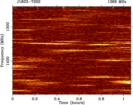
Figure 1: Dynamic spectrum of PSR J1603$-$7202 observed with the Parkes telescope on 2009 August 12.

3 Detecting pulsars in variance images

To investigate the detection of pulsars in variance images, it is important to understand the false alarm probability and the detection probability. In this section, through simulations and discussions of false alarm and detection probabilities, we aim to answer questions such as

• For a given survey with fixed total bandwidth, integration time, number of channels and subintegrations, how sensitive is it to pulsars with different scintillation time-scale and bandwidth?

• For a given survey with fixed total bandwidth and integration time, how does the sensitivity change with different numbers of channels and subintegrations?

In our simulations and discussions below, we consider a radio continuum image of a sky area containing a pulsar. The total integration time is $T$ and the total bandwidth is $B$. Each image pixel consists of $N_{\rm{t}}$ subintegrations and $N_{\rm{f}}$ channels, and therefore the subintegration time is $\delta t=T/N_{\rm{t}}$ and the channel bandwidth is $\delta\nu=B/N_{\rm{f}}$. The standard deviation of noise averaged over $T$ and $B$ is $\sigma_{\rm{n}}$, which gives the standard deviation of noise in each dynamic spectrum pixel of $\sigma_{\rm{dyn}}=\sigma_{\rm{n}}\sqrt{N}$ and $N=\sqrt{N_{\rm{f}}N_{\rm{t}}}$. The pulsar shows DISS with a scintillation time-scale of $\tau_{\rm{DISS}}$ and a scintillation bandwidth of $\delta\nu_{\rm{DISS}}$. In the dynamic spectrum the pulsar flux density as a function of time and frequency is $S_{\rm{dyn}}(t,\nu)$, and the mean of $S_{\rm{dyn}}(t,\nu)$ over the dynamic spectrum is $S_{\rm{psr}}$. All parameters are in arbitrary units.

To simulate the dynamic spectrum of the DISS we assume relatively strong scattering. In this case the electric field of the DISS is a complex Gaussian process where the real and imaginary parts are uncorrelated. Thus the auto-covariance (ACF) of the intensity is the square of the auto-covariance of the field. There is a simple and exact analytical expression for the temporal covariance but only an approximate expression for the frequency covariance (e.g., Coles et al., 2010). We have grafted those expressions together in a way that preserves the existence condition for an ACF, that its Fourier transform be positive semi-definite,

$$C(t,\nu)=\exp{\left(-\frac{1}{2}\left[(\frac{t}{\tau_{\rm{DISS}}})^{\frac{5}{2}}+(\frac{\nu}{\delta\nu_{\rm{DISS}}})^{\frac{3}{2}}\right]^{\frac{2}{3}}\right)}.$$ (3)

The ACF of intensity is the square of this, so the $1/\mathrm{e}$ time and frequency scales are $\tau_{\rm{DISS}}$ and $\delta\nu_{\rm{DISS}}$ respectively.

The Fourier transform of a Gaussian random process is also a Gaussian random process, so the Fourier transform of the electric field must be a Gaussian random process for which the expected value of the squared magnitude is the power spectrum $P$. We obtain $P$ from Fourier transformation of Eq. 3. We then create a realization of the electric field of the form $\sqrt{P/2}\cdot(a+\mathrm{i}b)$, where a and b are uncorrelated unit variance Gaussian random variables. The inverse transformation of this realization is the dynamic spectrum of the electric field $E(t,\nu)$, and its squared magnitude is a realization of the dynamic spectrum of intensity $I(t,\nu)=|E(t,\nu)|^{2}$.

This process provides a good approximation for most pulsars observed at centimetre or metre wavelengths. However it does not include the effects of enhanced refraction which are seen to cause correlation between the time and frequency variations in the dynamic spectrum. A more realistic simulation could be obtained with a full electromagnetic simulation (Coles et al., 2010), but such simulations would be difficult to extend to the very strong scintillation often seen at metre wavelengths.

3.1 Noise, false alarms and a “matched filter”

A detection is made when the detection statistic exceeds a threshold. The threshold is set so the probability that it is exceeded by noise alone is adequately small (of order per cent). Here we assume that noise is radiometer noise which is uncorrelated over the dynamic spectrum. The mean pulsar flux averaged over the dynamic spectrum $S_{\rm{psr}}$ gives a suitable detection statistic for continuum images or Stokes I images. The false alarm threshold would be a multiple of the standard deviation of the radiometer noise $\sigma_{n}$ averaged over the entire dynamic spectrum, i.e. detection is claimed if $S_{\rm{psr}}>C\cdot\sigma_{\rm{n}}$.

For a scintillating pulsar in variance images, detection would be claimed if

$$V_{\rm{psr}}=S_{\rm{psr}}^{2}>C\cdot\rm{Std}(\sigma_{\rm{dyn}}^{2}),$$ (4)

where $V_{\rm{psr}}$ is the mean of the sample variance of $S_{\rm{dyn}}(t,\nu)$ and equals to $S_{\rm{psr}}^{2}$ as $S_{\rm{dyn}}(t,\nu)$ follows an exponential distribution. If there are $N\gg 1$ independent samples in the dynamic spectrum and the radiometer noise is approximately Gaussian, the sample variance of $\sigma_{\rm{dyn}}^{2}$ computed over $N$ samples equals to $2N\cdot\sigma_{\rm{n}}^{4}$, and $\rm{Std}(\sigma_{\rm{dyn}}^{2})=\sigma_{\rm{n}}^{2}\sqrt{2N}$. Therefore, Eq. 4 gives a minimum detectable flux in a variance image of

$$S_{\rm{psr}}>\sqrt{C}\cdot\sigma_{\rm{n}}\cdot(2N)^{1/4}.$$ (5)

The ratio $R$ of the minimum detectable flux in a variance image to the minimum detectable flux in a Stokes I image is $R=(2N)^{0.25}/C^{0.5}$. So in forming a dynamic spectrum and calculating the variance of the flux, one should not use more samples than necessary. On the other hand, if one uses fewer samples than there are independent fluctuations (scintles) $N_{\rm{indep}}$ in the scintillating flux, then the variance of the flux will be reduced by a factor of $\sim N/N_{\rm{indep}}$ smoothing.

Clearly the optimal number of samples in the dynamic spectrum must be matched to the number of independent scintles in the scintillating flux. The time-scale and bandwidth of the DISS are auto-covariance widths. They should match the auto-covariance width of the sub-integration $\sim\delta t/2$ and the channel bandwidth $\sim\delta\nu/2$. To demonstrate the “matched filter”, we carry out simulations to show how $V_{\rm{psr}}/\rm{Std}(\sigma_{\rm{dyn}}^{2})$ varies with channel bandwidth and subintegration time. We set $T=100$, $B=100$, $\tau_{\rm{DISS}}=1$, $\nu_{\rm{DISS}}=1$, $S_{\rm{psr}}=10$ and $\sigma_{\rm{n}}=0.1$. In Fig. 2, for the blue solid line, we set $\delta t/2=\tau_{\rm{DISS}}=1$, which represents “matched filter” in time and gives a number of subintegrations of 50. We simulate a dynamic spectrum with 50 subintegrations and 10000 channels, and then average over different numbers of channels to produce dynamic spectra with different channel bandwidths. We simulate 10000 realisations and calculate the mean of sample variance for each channel bandwidth. We separately simulate the noise following the same procedure and calculate the standard deviation of sample variance for each channel bandwidth. For the red dashed line, we set $\delta\nu/2=\nu_{\rm{DISS}}=1$ and carry out similar simulations for different subintegration time. We can see in Fig. 2 that both solid and dashed lines peaks at $\sim 2$, which corresponds to the “matched filter” case that $\delta\nu/2\approx\delta\nu_{\rm{DISS}}$ and $\delta t/2\approx\tau_{\rm{DISS}}$.

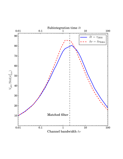
Figure 2: $V_{\rm{psr}}/\rm{Std}(\sigma_{\rm{dyn}}^{2})$ as a function of channel bandwidth and subintegration time for a given pulsar in the variance image. The scintillation time-scale and bandwidth of the pulsar are $\tau_{\rm{DISS}}=1$ and $\delta\nu_{\rm{DISS}}=1$, respectively. The total integration time and bandwidth are $T=100$ and $B=100$, respectively. The noise level is $\sigma_{\rm{n}}=0.1$ and pulsar apparent flux density is $S_{\rm{psr}}=10$. For the blue solid line we set $\delta t/2=\tau_{\rm{DISS}}=1$ and vary channel bandwidth, while for the red dashed line we set $\delta\nu/2=\nu_{\rm{DISS}}=1$ and vary subintegration time.

3.2 Detection probability

The detection probability is the probability of a signal exceeding the detection threshold. Different from that of a continuum source, the detection probability of a scintillating source will depend on its scintillation time-scale and bandwidth, and also on the integration time, bandwidth and time and frequency resolution of the survey. A useful way of understanding and investigating the detection probability is comparing the signal with its standard deviation. We can define the S/N of detecting a pulsar in Stokes I images as

$$(\mathrm{S/N})_{\mathrm{I}}=S_{\mathrm{psr}}/\mathrm{Std}(S_{\mathrm{psr}}),$$ (6)

and the S/N of detecting a pulsar in variance images as

$$(\mathrm{S/N})_{\mathrm{var}}=V_{\mathrm{psr}}/\mathrm{Std}(V_{\mathrm{psr}}).$$ (7)

Assuming that there are $N\gg 1$ independent samples in the dynamic spectrum and the noise is negligible, flux densities of a scintillating pulsar follow an exponential distribution, and we have

$$\mathrm{Std}(S_{\rm{psr}})=S_{\rm{psr}}/\sqrt{N},$$ (8)

$$\mathrm{Std}(V_{\rm{psr}})=\sqrt{\frac{(N-1)[(N-1)\mu_{4}-(N-3)\mu^{2}_{2}]}{N^{3}}}\approx\sqrt{8}\cdot S_{\rm{psr}}^{2}/\sqrt{N},$$ (9)

where $\mu_{4}=9S_{\rm{psr}}^{4}$ is the fourth central moment and $\mu_{2}=S_{\rm{psr}}^{2}$ is the second central moment. Therefore, (S/N)${}_{\rm{I}}=\sqrt{N}$ and (S/N)${}_{\rm{var}}=\sqrt{N/8}$, the detection possibility of a pulsar in variance images is a factor of $\sqrt{8}$ lower than that in Stokes I images. The underlying reason is that the variance of sample variance is larger than the variance of sample mean, and therefore the detection is more uncertain.

If the noise is not negligible, we find that the S/N of detecting pulsars in variance images drops faster than it does in Stokes I images as the noise level increases. In Fig. 3, we show how (S/N)_I and (S/N)_var vary with the noise level in the upper panel and the ratio between them in the bottom panel. We set $T=100$, $B=100$, $\delta t/2=\tau_{\rm{DISS}}=1$, $\delta\nu/2=\delta\nu_{\rm{DISS}}=1$ and $S_{\rm{psr}}=1$. For each noise level in the figure, we simulate a dynamic spectrum of the pulsar with noises and calculate the sample mean and the sample variance. We assume that we have ten image pixels to measure the noise level, and therefore we separately simulate dynamic spectra with only noise for each of these ten pixel. We calculate the mean of sample mean and the mean of sample variance for these ten pixels and subtract them from the pulsar signal to remove noises. For each noise level in the figure, we simulate $10000$ realisations of above simulations and then calculate $\mathrm{Std}(S_{\rm{psr}})$ and $\mathrm{Std}(V_{\rm{psr}})$. In Fig. 3 we can see that (S/N)_I is about a factor of $\sqrt{8}$ higher than (S/N)_var when the noise is negligible. As the noise becomes significant and increases, (S/N)_I/(S/N)_var drops rapidly, which means that the variance image becomes less and less sensitive than the Stokes I image as the noise increases.

We note that despite Stokes I images having higher sensitivity for detecting a pulsar, such images only provide limited information, e.g., the compactness, by which you can distinguish a pulsar from other radio sources. On the contrary, the DISS variance images are likely to allow exclusive detections of pulsars.

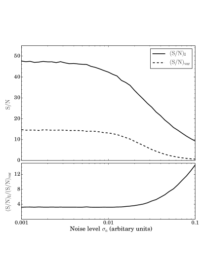
Figure 3: $(\rm{S/N})_{\rm{I}}$ and $(\rm{S/N})_{\rm{var}}$ as a function of noise level in the upper panel and the ratio between them in the bottom panel. Parameters of the simulation are $T=100$, $B=100$, $\delta t/2=\tau_{\rm{DISS}}=1$, $\delta\nu/2=\nu_{\rm{DISS}}=1$ and $S_{\rm{psr}}=1$.

3.3 Detection sensitivity of pulsars in variance images

To define the detection of a pulsar in variance images, we first determine the detection threshold as the value that is exceeded in only five per cent of the noise, which corresponds to a five per cent false alarm probability. Then we determine the flux density of a pulsar with which 80 per cent of the measurements exceed the detection threshold. We define such a flux density as the sensitivity of a survey with a five per cent false alarm probability and 80 per cent detection probability. Same detection statistics can also be defined for Stokes I images.

We simulate dynamic spectra with noises to obtain the distributions of both mean flux density and variance of flux density of pulsars, and we separately simulate the noise distributions without pulsar signals. In Fig. 4, we show an example of the distributions with 10000 simulations. We set $T=100$, $B=100$, $N_{\rm{t}}=10$, $N_{\rm{f}}=10$, $\tau_{\rm{DISS}}=1$ and $\delta\nu_{\rm{DISS}}=1$. The pulse flux density is set to be $S_{\rm{psr}}=1.5$ and the noise level is $\sigma_{\rm{n}}=0.2$. The left panel shows results of variance images and the right panel shows results of Stokes I images. The green dashed line represents a detection threshold corresponding to five per cent false alarm probability. From the distributions we can see that, for the same false alarm probability, Stokes I images have a higher detection probability compared with variance images, which is consistent with our discussions in Section 3.1 and 3.2.

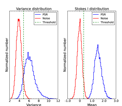
Figure 4: Histograms of noise and pulsar intensities. The green dashed line shows the detection threshold corresponding to five per cent false alarm probability. Parameters of the simulations are $T=100$, $B=100$, $N_{\rm{t}}=10$, $N_{\rm{f}}=10$. $\tau_{\rm{DISS}}=1$ and $\delta\nu_{\rm{DISS}}=1$. The pulse flux density is set to be $S_{\rm{psr}}=1.5$ and the noise level is $\sigma_{\rm{n}}=0.2$.

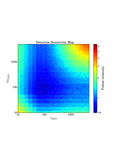
Figure 5: Sensitivity map as a function of scintillation time-scale $\tau_{\rm{DISS}}$ and bandwidth $\delta\nu_{\rm{DISS}}$. Sensitivity are shown as the intensity in arbitrary units corresponding to a detection probability of 80% and a false alarm probability of 5%. Parameters of the simulation are $T=1000$, $B=1000$, $N_{\rm{t}}=10$, $N_{\rm{f}}=10$ and $\sigma_{\rm{n}}=0.1$. The sensitivity of a Stokes image with the same parameters is $\sim 0.25$.

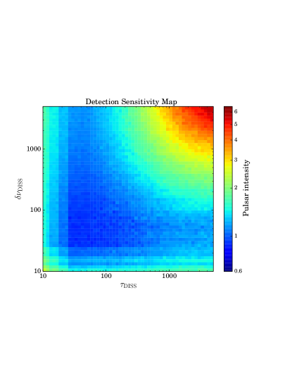
Figure 6: Same as Fig. 5 but with $N_{\rm{t}}=20$ and $N_{\rm{f}}=20$.

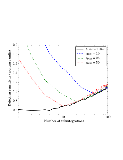
Figure 7: Detection sensitivity as a function of number of subintegrations for a given total integration time. Parameters of the simulation are the same as those of Fig. 5. For the solid line, we set $\tau_{\rm{DISS}}=\delta t/2$ and the subintegration time varies as $\delta t=T/N_{\rm{t}}$. We also set $\delta\nu_{\rm{DISS}}=\delta\nu/2=50$. For the dashed, dash-dotted and dotted line, we set $\delta\nu_{\rm{DISS}}$=10, 25 and 50, respectively.

With the detection defined above, we carry out simulations to investigate the sensitivity of a given survey to pulsars with different scintillation bandwidth and time-scale. We assume that the survey has $T=1000$, $B=1000$ and $\sigma_{\rm{n}}=0.1$. In Fig. 5, we set $N_{\rm{f}}=10$ and $N_{\rm{t}}=10$, while in Fig. 6 we set $N_{\rm{f}}=20$ and $N_{\rm{t}}=20$. The colour scale of two figures are the same. Both figures show that variance images are sensitive to pulsars whose $\delta\nu_{\rm{DISS}}$ and $\tau_{\rm{DISS}}$ are close to $\delta\nu/2$ and $\delta t/2$, and the sensitivity drops quickly as $\delta\nu_{\rm{DISS}}$ and $\tau_{\rm{DISS}}$ get much smaller or larger than $\delta\nu$ and $\delta t$. Comparing Fig. 5 with Fig. 6, we can see that for a given total bandwidth $B$ and integration time $T$, when we increase the number of channels and subintegrations we become relatively more sensitive to pulsars with small $\delta\nu_{\rm{DISS}}$ and $\tau_{\rm{DISS}}$, and lose sensitivity to pulsars with large $\delta\nu_{\rm{DISS}}$ and $\tau_{\rm{DISS}}$. With the same simulation, we can also determine the sensitivity of a Stokes I image with five per cent false alarm probability and 80 per cent detection probability. We obtained a sensitivity of Stokes I image of $\sim 0.25$ for the same simulation parameters, which is independent of scintillation time-scale and bandwidth and time and frequency resolutions.

However, for a given total bandwidth and integration time, as we increase the number of channels and subintegrations the noise level in the dynamic spectrum increases and we lose sensitivity as discussed in Section 3.2. In Fig. 7, we show the detection sensitivities of the “matched filter” case as a function of the number of subintegrations for a given total integration time. Parameters of simulations are the same as Fig. 5. We set $\tau_{\rm{DISS}}=\delta t/2$ and the subintegration time varies as $\delta t=T/N_{\rm{t}}$. We also set $\delta\nu_{\rm{DISS}}=\delta\nu/2=50$ and other parameters same as those of Fig. 5. The solid line represents the “matched filter” case, and in comparison we also present the detection sensitivity of cases that have fixed scintillation time-scales with dashed, dash-dotted and dotted lines. For the “matched filter” case, which gives us the highest sensitivity for different numbers of subintegrations, we can see that the sensitivity decreases as the number of subintegrations increases. For other cases, the highest sensitivities appear when $\tau_{\rm{DISS}}\approx\delta t/2$, which is consistent with Fig. 2.

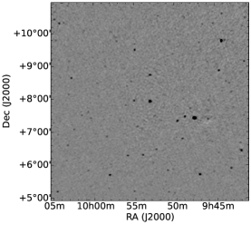
(a)

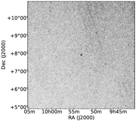
(b)

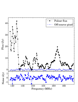
(c)

Figure 8: Demonstration of the variance imaging technique. (a) shows the Stokes I image with PSR J0953$+$0755 in the centre. (b) shows the variance image of the same field. (c) shows the flux densities of PSR J0953$+$0755 and an off-source image pixel as a function of frequency averaged over the 112 second snapshot in the upper panel. The bottom panel of (c) shows a zoom-in of flux densities of the off-source pixel. For details of the data set see Bell et al. (2016).

4 Demonstration of the technique

To demonstrate that we can detect scintillating pulsars in variance images and distinguish them from other radio sources, we use data taken with MWA (Tingay et al., 2013). For the pulsar PSR J0953$+$0755, Bell et al. (2016) report variability in a time series of images taken over a period of approximately 30 minutes. The data were taken at a central frequency of 154 MHz with a bandwidth of 30.72 MHz. For a full discussion of the pulsar variability survey and associated data acquisition and reduction methodology see Bell et al. (2016). Here we examined a single 112 second MWA snapshot of PSR J0953$+$0755 whilst undergoing diffractive scintillation. The data were re-imaged at 1 MHz spectral resolution. Bell et al. (2016) measure a scintillation bandwidth $\delta\nu_{\rm{DISS}}$ of 4.1 MHz and scintillation time-scale $\tau_{\rm{DISS}}$ of 28.8 minutes. The scintillation pattern in time is therefore not resolved, but the 1 MHz channels are adequate to sample significant frequency fluctuations with width of order 4 MHz.

Fig. 8 shows on the left panel a Stokes I image made using the full 30.72 MHz bandwidth. The middle panel shows the variance image made with 1 MHz channel bandwidth. To make the variance image, we have applied a sub-band subtraction filter, where by adjacent channels are subtracted. Such a filter removes signals that show slow and smooth fluctuations as a function of frequency, including signals from radio sources with non-flat spectra and instrumental effects associated with the bandpass and so on. This filter also reduces the S/N of pulsars in the variance image, especially when the scintillation is over-sampled in frequency, since fluctuations between channels are reduced when the channel bandwidth is narrower than the scintillation bandwidth. In the Stokes I image, we can see a number of strong point-like radio sources, which are difficult to be distinguished from pulsars without additional information. In contrast, in the variance image PSR J0953$+$0755 can be clearly identified and is the only source in the image.

The right panel of Fig. 8 shows the flux density of PSR J0953$+$0755 as a function of frequency averaged over the 112 second snapshot. In comparison, we also show the flux density of an off-source image pixel as a function of frequency in the upper panel and its zoom-in in the bottom panel. The flux densities are measured from images without any deconvolution and cleaning, and the frequency resolution of $\sim$160 kHz is much smaller than the scintillation bandwidth. We clearly see the modulation caused by DISS and structures with frequency scale of $\sim 4$ MHz. A full dynamic spectrum over 30 minutes has been presented in Bell et al. (2016). In Fig. 9, the upper and bottom panels show $V_{\rm{psr}}$ and $\sqrt{V_{\rm{psr}}/\rm{Std}(\sigma_{\rm{dyn}}^{2})}$ as a function of channel bandwidth, respectively. Blue points show results without sub-band subtraction while red points are results after sub-band subtraction. Without sub-band subtraction, as the channel bandwidth decreases we over-sample the scintillation and the variance saturates. After sub-band subtraction the variance decreases as the channel bandwidth decreases, and it peaks at around the scintillation bandwidth. Since we cannot resolve the scintillation in time and the observing bandwidth is only $\sim 7$ times of the scintillation bandwidth, we see significant fluctuations in $V_{\rm{psr}}$ as we average the flux over different channel bandwidth. To estimate $\sqrt{V_{\rm{psr}}/\rm{Std}(\sigma_{\rm{dyn}}^{2})}$, we assume that the noise is Gaussian and $\rm{Std}(\sigma_{\rm{dyn}}^{2})=\sigma_{\rm{n}}^{2}\cdot\sqrt{2N}$. $\sigma_{\rm{n}}$, as the standard deviation of noise in the Stokes I image averaged over 30.72 MHz bandwidth, is measured to be $\sim 0.075$ Jy. $\sqrt{V_{\rm{psr}}/\rm{Std}(\sigma_{\rm{dyn}}^{2})}$ for both with and without sub-band subtraction cases peak at around a channel bandwidth of $\sim 5$ MHz, close to the “matched filter” of $\delta\nu/2=\delta\nu_{\rm{DISS}}$ as we discussed in Section 3.1 and 3.2.

We have assumed that the noise in the image is radiometer noise and is stationary over the image. This is a reasonable assumption at centimetre wavelengths but not at meter wavelengths. For MWA the system temperature is dominated by the Galactic background and is not stationary over the field of view of the image. Incomplete correction of sidelobes of strong sources will not scintillate in time but they might show some variation in frequency which could be interpreted as scintillation. We have used PSR J0953$+$0755 as an example to show the feasibility of detecting pulsars with significant DISS in variance images. Studies of the noise properties and imaging technique are beyond the scope of this work, though they are of great importance for applying variance images in pulsar searching.

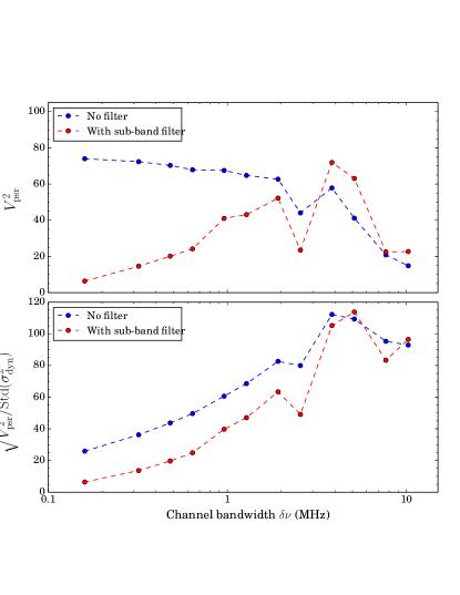
Figure 9: Upper panel: $V_{\rm{psr}}$ as a function of channel bandwidth. Bottom panel: $\sqrt{V_{\rm{psr}}/\rm{Std}(\sigma_{\rm{dyn}}^{2})}$ as a function of channel bandwidth. Blue points show results without sub-band subtraction while red points are results after sub-band subtraction.

5 Discussion and Conclusions

We investigated the variation of pulsar intensity caused by DISS in variance images. Through simulations, we studied the sensitivity of variance images on detecting pulsars and compared it with Stokes I images. Using data taken with MWA, we demonstrated that variance images can lead to the detection of pulsars and distinguish pulsars from other radio sources. We conclude that DISS of pulsars provides us with a unique way to distinguish pulsars from other radio sources. With the variance imaging technique, we will be able to select the most promising pulsar candidates from large-scale continuum surveys and enhance the efficiency of following targeted search.

Variance images are most sensitive to pulsars whose scintillation bandwidth and time-scales are close to the channel bandwidth and subintegration time. Therefore, for a given continuum survey with certain total bandwidth and integration time, in order to achieve the highest sensitivity and detect as many pulsars as possible, we will need to retain frequency and time resolution as high as possible, and construct a set of variance images with different channel bandwidth and subintegration time. Typically the time scale is not a problem but it is common for the channel bandwidth to limit the detection of scintillation. On the other hand, increasing time and frequency resolution will decrease the overall sensitivity of variance images because the noise level in each channel and subintegration increases. This indicates that, for a given total bandwidth and integration time, variance images will be relatively less sensitive to pulsars with small scintillation bandwidth and time-scales.

The sensitivity maps presented in the paper and simulations we developed can be used to predict the number of pulsars detectable with variance images for future large-scale continuum surveys, e.g., MWATS, EMU and SKA. Taking the sensitivity of EMU ($\sim 10$ $\mu$Jy) as an example, assuming we have enough bandwidth and time and frequency resolution to detect pulsar scintillation, the sensitivity of variance images constructed with EMU will be $\sim 60$ to 100 $\mu$Jy, depending on the time and frequency resolution. To determine the number of pulsars that can be detected, pulsar Galactic and flux density distributions and their scintillation time-scales and bandwidths will have to be considered. We defer studies of pulsar population and prediction of pulsar detection with variance images to future work.

Although variance images allow unique identifications of pulsars, for given false alarm and detection probabilities, the sensitivity of variance images is lower than that of Stokes I images. Therefore, very faint pulsars detectable in continuum surveys might not be identified in variance images even if they show strong scintillation. However, the diffractive scintillation features of pulsars can still be powerful criteria to distinguish them from other radio sources. Instead of making variance images, we could first identify point sources in continuum surveys and then use scintillation features to distinguish pulsars from other sources.

References

- Backer et al. (1982) Backer D. C., Kulkarni S. R., Heiles C., Davis M. M., Goss W. M., 1982, Nature, 300, 615
- Bell et al. (2016) Bell M. E., et al., 2016, ArXiv:1605.09100,
- Bowman et al. (2013) Bowman J. D., et al., 2013, Publ. Astron. Soc. Australia, 30, e031
- Coles (1995) Coles W. A., 1995, Space Sci. Rev., 72, 211
- Coles et al. (2010) Coles W. A., Rickett B. J., Gao J. J., Hobbs G., Verbiest J. P. W., 2010, ApJ, 717, 1206
- Cordes & Rickett (1998) Cordes J. M., Rickett B. J., 1998, ApJ, 507, 846
- Crawford et al. (1996) Crawford D. F., Robertson J. G., Davidson G., 1996, MNRAS, 283, 336
- Crawford et al. (2000) Crawford F., Kaspi V. M., Bell J. F., 2000, AJ, 119, 2376
- Dai et al. (2015) Dai S., et al., 2015, MNRAS, 449, 3223
- Faucher-Giguère & Kaspi (2006) Faucher-Giguère C.-A., Kaspi V. M., 2006, ApJ, 643, 332
- Goodman & Narayan (1985) Goodman J., Narayan R., 1985, MNRAS, 214, 519
- Han & Tian (1999) Han J. L., Tian W. W., 1999, A&AS, 136, 571
- Heald et al. (2015) Heald G. H., et al., 2015, A&A, 582, A123
- Hotan et al. (2004) Hotan A. W., van Straten W., Manchester R. N., 2004, Publ. Astron. Soc. Australia, 21, 302
- Kaplan et al. (1998) Kaplan D. L., Condon J. J., Arzoumanian Z., Cordes J. M., 1998, ApJS, 119, 75
- Kaplan et al. (2000) Kaplan D. L., Cordes J. M., Condon J. J., Djorgovski S. G., 2000, ApJ, 529, 859
- Keith et al. (2013) Keith M. J., et al., 2013, MNRAS, 429, 2161
- Kouwenhoven (2000) Kouwenhoven M. L. A., 2000, A&AS, 145, 243
- Loi et al. (2015) Loi S. T., et al., 2015, MNRAS, 453, 2731
- Manchester et al. (2013) Manchester R. N., et al., 2013, Publ. Astron. Soc. Australia, 30, 17
- Narayan (1992) Narayan R., 1992, Philosophical Transactions of the Royal Society of London Series A, 341, 151
- Norris et al. (2011) Norris R. P., et al., 2011, Publ. Astron. Soc. Australia, 28, 215
- Rickett (1977) Rickett B. J., 1977, ARA&A, 15, 479
- Rickett (1990) Rickett B. J., 1990, ARA&A, 28, 561
- Tingay et al. (2013) Tingay S. J., et al., 2013, Publ. Astron. Soc. Australia, 30, e007