Test Models for Statistical Inference: Two-Dimensional Reaction Systems Displaying Limit Cycle Bifurcations and Bistability

Abstract

Theoretical results regarding two-dimensional ordinary-differential equations (ODEs) with second-degree polynomial right-hand sides are summarized, with an emphasis on limit cycles, limit cycle bifurcations and multistability. The results are then used for construction of two reaction systems, which are at the deterministic level described by two-dimensional third-degree kinetic ODEs. The first system displays a homoclinic bifurcation, and a coexistence of a stable critical point and a stable limit cycle in the phase plane. The second system displays a multiple limit cycle bifurcation, and a coexistence of two stable limit cycles. The deterministic solutions (obtained by solving the kinetic ODEs) and stochastic solutions (noisy time-series generating by the Gillespie algorithm, and the underlying probability distributions obtained by solving the chemical master equation (CME)) of the constructed systems are compared, and the observed differences highlighted. The constructed systems are proposed as test problems for statistical methods, which are designed to detect and classify properties of given noisy time-series arising from biological applications.

1 Introduction

Given noisy time-series, it may be of practical importance to infer possible biological mechanisms underlying the time-series [1]. Mathematically, such statistical inferences correspond to an inverse problem, consisting of mapping given noisy time-series to compatible reaction networks. One way to formulate the inverse problem is as follows. Firstly, one obtains deterministic kinetic ordinary-differential equations (ODEs) compatible with the stochastic time-series. And secondly, suitable reaction networks may then be induced from the obtained kinetic ODEs [2, 3]. The inverse problem is generally ill-posed [2, 3], as more than one suitable reaction networks may be obtained. In order to make a progress in solving the inverse problem, it is useful to impose further constraints on the kinetic ODEs. A particular set of constraints on the kinetic ODEs may be obtained by determining the types of the deterministic attractors which are ‘hidden’ in the noisy time-series [1]. This may be a challenging task, especially when cycles (oscillations) are observed in the time-series. The observed cycles may be present in both the deterministic and stochastic models (also known at the stochastic level as noisy deterministic cycles), or they may be present only in the stochastic model (also known as quasi-cycles, or noise-induced oscillations). Noisy deterministic cycles may arise directly from the autonomous kinetic ODEs, or via the time-periodic terms present in the nonautonomous kinetic ODEs. Quasi-cycles may arise from the intrinsic or extrinsic noise, and have been shown to exist near deterministic stable foci, and stable nodes [4]. For two-species reaction systems, quasi-cycles can be further classified into those that are unconditionally noise-dependent (but dependent on the reaction rate coefficients), and those that are conditionally noise-dependent [4]. Thus, a cycle detected in a noisy time-series may at the deterministic level generally correspond to a stable limit cycle, a stable focus, or a stable node.

In order to detect and classify cycles in noisy time-series, several statistical methods have been suggested [1, 5]. In [1], analysis of the covariance as a function of the time-delay, spectral analysis (the Fourier transform of the covariance function), and analysis of the shape of the stationary probability mass function, have been suggested. Let us note that reaction systems of the Lotka-Volterra ($x$-factorable [2]) type are used as test models in [1], and that conditionally noise-dependent quasi-cycles, which can arise near a stable node, and which can induce oscillations in only a subset of species [4], have not been discussed. In addition to the aforementioned statistical methods developed for analysing noisy time-series, methods for (locally) studying the underlying stochastic processes near the deterministic attractors/bifurcations have also been developed [4, 6, 7, 8, 9, 10, 11].

Statistical and analytical methods for studying cycles in stochastic reaction kinetics have often been focused on deterministically monostable systems which undergo a local bifurcation near a critical (equilibrium) point, known as the supercritical Hopf bifurcation. We suspect this is partially due to simplicity of the bifurcation, and partially due to the fact that it is difficult to find two-species reaction systems, which are more amenable to mathematical analysis, undergoing more complicated bifurcations and displaying bistability involving limit cycles. Nevertheless, kinetic ODEs arising from biological applications may exhibit more complicated bifurcations and multistabilites [12, 13, 14]. Thus, it is of importance to test the available methods on simpler test models that display some of the complexities found in the applications.

In this paper, we construct two reaction systems that are two-dimensional (i.e. they only include two chemical species) and induce cubic kinetic equations, first of which undergoes a global bifurcation known as a convex supercritical homoclinic bifurcation, and which displays bistability involving a critical point and a limit cycle (which we call mixed bistability). The second system undergoes a local bifurcation known as a multiple limit cycle bifurcation, and displays bistability involving two limit cycles (which we call bicyclicity). Aside from finding an application as test models for statistical inference and analysis in biology, to our knowledge, the constructed systems are also the first examples of two-dimensional reaction systems displaying the aforementioned types of bifurcations and bistabilities. Let us note that reaction systems with dimensions higher than two, displaying the homoclinic bifurcation, as well as bistabilities involving two limit cycles, have been reported in applications [12, 13, 14].

The reaction network corresponding to the first system is given by

$$r_{1}:\; \varnothing \xrightarrow[]{k_{1}}s_{1},\;\;\;\;\;\;\;\;\;\;\;\;\;\;\;\;\;\;\;\;\;\;\;\;\;\;\;\;\;\;\;\;\;\;\,r_{7}: \varnothing \xrightarrow[]{k_{7}}s_{2},$$

$$r_{2}:\; s_{1} \xrightarrow[]{k_{2}}2s_{1},\;\;\;\;\;\;\;\;\;\;\;\;\;\;\;\;\;\;\;\;\;\;\;\;\;\;\;\;\;\;\;\;\,r_{8}: s_{2} \xrightarrow[]{k_{8}}\varnothing,$$

$$r_{3}:\; 2s_{1} \xrightarrow[]{k_{3}}3s_{1},\;\;\;\;\;\;\;\;\;\;\;\;\;\;\;\;\;\;\;\;\;\;\;\;\;\;\;\;\;\;\;\;\,r_{9}: s_{1}+s_{2} \xrightarrow[]{k_{9}}s_{1}+2s_{2},$$

$$r_{4}:\; s_{1}+s_{2} \xrightarrow[]{k_{4}}s_{2},\;\;\;\;\;\;\;\;\;\;\;\;\;\;\;\;\;\;\;\;\;\;\;\;\;\;\;\;\;\;\;\;\;r_{10}: 2s_{2} \xrightarrow[]{k_{10}}3s_{2},$$

$$r_{5}:\; 2s_{1}+s_{2} \xrightarrow[]{k_{5}}s_{1}+s_{2},\;\;\;\;\;\;\;\;\;\;\;\;\;\;\;\;\;\;\;\;\;\;\;\;\;\,r_{11}: 3s_{2} \xrightarrow[]{k_{11}}2s_{2},$$

$$r_{6}:\; s_{1}+2s_{2} \xrightarrow[]{k_{6}}2s_{1}+2s_{2},$$ (1)

where the two species $s_{1}$ and $s_{2}$ react according to the eleven reactions $r_{1},r_{2},\ldots,r_{11}$ under mass-action kinetics, with the reaction rate coefficients denoted $k_{1},k_{2},\ldots,k_{11}$, and with $\varnothing$ being the zero-species [2]. A particular choice of the (dimensionless) reaction rate coefficients is given by

$$k_{1} =0.01,\;\;\;k_{2}=0.9,\;\;\;k_{3}=1.55,\;\;\;k_{4}=2.6,\;\;\;k_{5}=1.2,\;\;\;k_{6}=1.5,$$

$$k_{7} =0.01,\;\;\;k_{8}=3.6,\;\;\;k_{9}=1,\;\;\;k_{10}=2.4,\;\;\;k_{11}=0.8,$$ (2)

while more general conditions on these parameters are derived later as equations (10) and (11).

The reaction network corresponding to the second system includes two species $s_{1}$ and $s_{2}$ which are subject the following fourteen chemical reactions $r_{1},r_{2},\ldots,r_{14}$:

$$r_{1}:\; \varnothing \xrightarrow[]{k_{1}}s_{1},\;\;\;\;\;\;\;\;\;\;\;\;\;\;\;\;\;\;\;\;\;\;\;\;\;\;\;\;\;\;\;\;\;\,r_{8}: \varnothing \xrightarrow[]{k_{8}}s_{2},$$

$$r_{2}:\; s_{1} \xrightarrow[]{k_{2}}\varnothing,\;\;\;\;\;\;\;\;\;\;\;\;\;\;\;\;\;\;\;\;\;\;\;\;\;\;\;\;\;\;\;\;\;\;r_{9}: s_{2} \xrightarrow[]{k_{9}}2s_{2},$$

$$r_{3}:\; 2s_{1} \xrightarrow[]{k_{3}}3s_{1},\;\;\;\;\;\;\;\;\;\;\;\;\;\;\;\;\;\;\;\;\;\;\;\;\;\;\;\;\;\;\,r_{10}: s_{1}+s_{2} \xrightarrow[]{k_{10}}s_{1},$$

$$r_{4}:\; s_{1}+s_{2} \xrightarrow[]{k_{4}}2s_{1}+s_{2},\;\;\;\;\;\;\;\;\;\;\;\;\;\;\;\;\;\;\;\;\;\;\;r_{11}: 2s_{2} \xrightarrow[]{k_{11}}3s_{2},$$

$$r_{5}:\; 3s_{1} \xrightarrow[]{k_{5}}4s_{1},\;\;\;\;\;\;\;\;\;\;\;\;\;\;\;\;\;\;\;\;\;\;\;\;\;\;\;\;\;\;\;r_{12}: 2s_{1}+s_{2} \xrightarrow[]{k_{12}}2s_{1}+2s_{2},$$

$$r_{6}:\; 2s_{1}+s_{2} \xrightarrow[]{k_{6}}s_{1}+s_{2},\;\;\;\;\;\;\;\;\;\;\;\;\;\;\;\;\;\;\;\;\;\;\;\;\;r_{13}: s_{1}+2s_{2} \xrightarrow[]{k_{13}}s_{1}+s_{2},$$

$$r_{7}:\; s_{1}+2s_{2} \xrightarrow[]{k_{7}}2s_{2},\;\;\;\;\;\;\;\;\;\;\;\;\;\;\;\;\;\;\;\;\;\;\;\;\;\;\;\;\;\;\;r_{14}: 3s_{2} \xrightarrow[]{k_{14}}2s_{2},$$ (3)

where $k_{1},k_{2},\ldots,k_{14}$ are the corresponding reaction rate coefficients. A particular choice of the (dimensionless) reaction coefficients is given by

$$k_{1} =2\times 10^{-7},\;\;\;k_{2}=19.987880407,\;\;\;k_{3}=0.019944378,$$

$$k_{4} =0.02003132232,\;\;\;k_{5}=2.9\times 10^{-8},\;\;\;k_{6}=2.000232\times 10^{-5},$$

$$k_{7} =1.45\times 10^{-8},\;\;\;k_{8}=2\times 10^{-7},\;\;\;k_{9}=8.38734,\;\;\;k_{10}=0.038389,$$

$$k_{11} =0.0215726,\;\;\;k_{12}=2\times 10^{-5},\;\;\;k_{13}=1.571\times 10^{-6},\;\;\;k_{14}=10^{-5},$$ (4)

while the general conditions on these parameters are given later as equations (13) and (14).

In Figure 1, we display a representative noisy-time series generated using the Gillespie stochastic algorithm, in Figure 1(a) for the one-dimensional cubic Schlögl system [15], which deterministically displays two stable critical points (bistationarity [3]), in Figure 1(b) for the reaction network (1) with coefficients (2), which deterministically displays a stable critical point and a stable limit cycle (mixed bistability), and in Figure 1(c) for the reaction network (3) with coefficients (4), which deterministically displays two stable limit cycles (bicyclicity). Several statistical challenges arise. For example, is it possible to infer that the upper attractor in Figure 1(b) is a deterministic critical point, while the lower a noisy limit cycle? Is it possible to detect one/both noisy limit cycles in Figure 1(c)? The answer to the second question is complicated by the fact that the two deterministic limit cycles in Figure 1(c) are relatively close to each other.

 

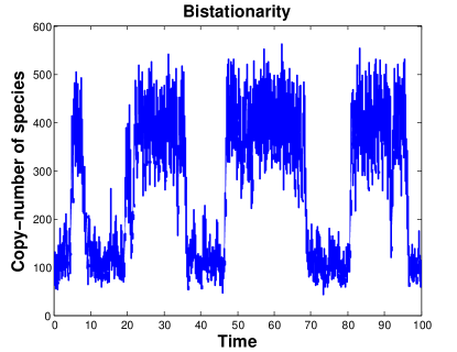
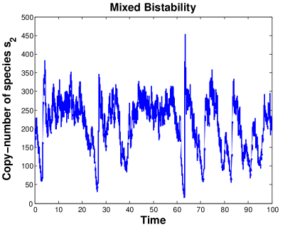
(a)                                                    (b)

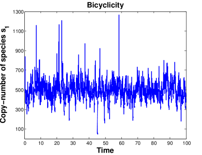
                        (c)

Figure 1: Panels (a), (b) and (c) show representative sample paths generated using the Gillespie stochastic simulation algorithm for the Schlögl system [15] with coefficients as in [6], reaction network $(\ref{eq:homoclinic1net})$ with coefficients $(\ref{eq:homoclinic1example})$ and reactor volume $V=100$, and reaction network $(\ref{eq:bicyclicXT2net})$ with coefficients $(\ref{eq:bicyclicexample})$ and $V=0.5$, respectively. At the deterministic level, the phase planes of $(\ref{eq:homoclinic1net})$ and $(\ref{eq:bicyclicXT2net})$ are shown in Figure 2. The deterministic and stochastic time-series, as well as the probability distributions, are shown in Figures 3 and 4. At the deterministic level, a critical point and a limit cycle are ‘hidden’ in (b), while two limit cycles are ‘hidden’ in (c).

The rest of the paper is organized as follows. In Section 2, we outline properties of the planar quadratic ODE systems, concentrating on cycles, cycle bifurcations and multistability. There are two reasons for focusing on the planar quadratic systems: firstly, the phase plane theory for such systems is well-developed [16, 17], with a variety of concrete examples with interesting phase plane configurations [18, 19, 20]. Secondly, an arbitrary planar quadratic ODE system can always be mapped to a kinetic one using only an affine transformation - a special property not shared with cubic (nor even linear) planar systems [21]. This, together with the available nonlinear kinetic transformations which increase the polynomial degree of an ODE system by one [2], imply that we may map a general planar quadratic system to at most cubic planar kinetic system, which may still be biologically or chemically relevant. In Section 3, we present the two planar cubic test models which induce reaction networks (1) and (3), and which are constructed starting from suitable planar quadratic ODE systems. We also compare the deterministic and stochastic solutions of the constructed reaction networks, and highlight the observed qualitative differences. Finally, in Section 4, we provide a summary of the paper.

2 Properties of two-dimensional second-degree polynomial ODEs: cycles, cycle bifurcations and multistability

Let us consider the two-dimensional second-degree autonomous polynomial ODEs

$$\frac{\mathrm{d}x_{1}}{\mathrm{d}t} =\mathcal{P}_{1}(x_{1},x_{2};\,\mathbf{k})=k_{1}+k_{2}x_{1}+k_{3}x_{2}+k_{4}x_{1}^{2}+k_{5}x_{1}x_{2}+k_{6}x_{2}^{2},$$

$$\frac{\mathrm{d}x_{2}}{\mathrm{d}t} =\mathcal{P}_{2}(x_{1},x_{2};\,\mathbf{k})=k_{7}+k_{8}x_{1}+k_{9}x_{2}+k_{10}x_{1}^{2}+k_{11}x_{1}x_{2}+k_{12}x_{2}^{2},$$ (5)

where $\mathcal{P}_{i}(\,\cdot\,,\,\cdot\,;\,\mathbf{k}):\mathbb{R}^{2}\to\mathbb{R}$, $i\in\{1,2\},$ are the second-degree two-variable polynomial functions, and $\mathbf{k}=(k_{1},k_{2},\dots,k_{12})\in\mathbb{R}^{12}$ is the vector of the corresponding coefficients. We assume that $\mathcal{P}_{1}$ and $\mathcal{P}_{2}$ are relatively prime and at least one is of second-degree. We allow coefficients $\mathbf{k}$ to be parameter-dependent, $\mathbf{k}=\mathbf{k}(\mathbf{p})$, with $\mathbf{p}\in\mathbb{R}^{q}$, $q\geq 0$.

Let us consider two additional properties which system (5) may satisfy:

1. Coefficients $k_{1},$ $k_{3},$ $k_{6},$ $k_{7},$ $k_{8},$ $k_{10}\geq 0$, i.e. $\mathcal{P}_{1}$ and $\mathcal{P}_{2}$ are so-called kinetic functions (for a rigorous definition see [2]).

2. The species concentrations $x_{1}=x_{1}(t)$ and $x_{2}=x_{2}(t)$ are uniformly bounded in time for $t\geq 0$ in the nonnegative orthant $\mathbb{R}_{\geq}^{2}$, except possibly for initial conditions located on a finite number of one-dimensional subsets of $\mathbb{R}_{\geq}^{2}$, where infinite-time blow-ups are allowed.

The subset of equations (5) satisfying properties (I)–(II) are referred to as the deterministic kinetic equations bounded in $\mathbb{R}_{\geq}^{2}$, and denoted

$$\frac{\mathrm{d}x_{1}}{\mathrm{d}t} =\mathcal{K}_{1}(x_{1},x_{2};\,\mathbf{k}(\mathbf{p})),$$

$$\frac{\mathrm{d}x_{2}}{\mathrm{d}t} =\mathcal{K}_{2}(x_{1},x_{2};\,\mathbf{k}(\mathbf{p})).$$ (6)

In what follows, we discuss only the biologically/chemically relevant solutions of (6), i.e. the solutions in the nonnnegative quadrant $\mathbb{R}_{\geq}^{2}$. We now summarize some of the definitions and results regarding cycles, cycle bifurcations and multistability (referred to as the so-called exotic phenomena in the biological context [3]) for systems (5) and (6). Let us note that most of the results have been shown to hold only for the more general system (5), and may not necessarily hold for the more restricted system (6).

Critical points. A (finite) critical point $(x_{1}^{*}(\mathbf{k}),x_{2}^{*}(\mathbf{k}))$ of system (5) is a solution of the polynomial system $\mathcal{P}_{1}(x_{1}^{*},x_{2}^{*};\,\mathbf{k})=0,\mathcal{P}_{2}(x_{1}^{*},x_{2}^{*};\,\mathbf{k})=0$. Critical points are the time-independent solutions of (5).

Cycles. Cycles of (5) are closed orbits in the phase plane which are not critical points. They can be isolated (limit cycles, and separatrix cycles) or nonisolated (a one-parameter continuous family of cycles). Limit cycles are the periodic solutions of (5). A homoclinic separatrix cycle consists of a homoclinic orbit and a critical point of saddle type, with the orbit connecting the saddle to itself. On the other hand, a heteroclinic separatrix cycle consists of two heteroclinic orbits, and two critical points, with the orbits connecting the two critical points [22]. Limit cycles of (6) correspond to biological clocks, which play an important role in fundamental biological processes, such as the cell cycle, the glycolytic cycle and circadian rhythms [23, 24, 25].

Cycle bifurcations. Variations of coefficients $\mathbf{k}$ in (5) may lead to changes in the topology of the phase plane (e.g. a change may occur in the number of invariant sets or their stability, shape of their region of attraction or their relative position). Variation of $\mathbf{k}(\mathbf{p})$ in (6) may be interpreted as a variation of the reaction rate coefficients $\mathbf{k}$ due to changes in the reactor (environment) parameters $\mathbf{p}$, such as the pressure or temperature. If the variation causes the system to become topologically nonequivalent, such a parameter is called a bifurcation parameter, and at the parameter value where the topological nonequivalence occurs, a bifurcation is said to take place [26, 22]. Bifurcations in the deterministic kinetic equations have been reported in applications [23, 24, 25, 27, 28, 12].

Bifurcations of limit cycles of (5) can be classified into three categories: (i) the Andronov-Hopf bifurcation, where a limit cycle is created from a critical point of focus or center type, (ii) the separatrix cycle bifurcation, where a limit cycle is created from a separatrix cycle, and (iii) the multiple limit cycle bifurcation, where a limit cycle is created from a limit cycle of multiplicity greater than one [16, 22]. Let us note that the maximum multiplicity of a multiple focus of (5) is three, so that at most three local limit cycles can be created under appropriate perturbations [29]. Bifurcations (i) and (iii) are examples of local bifurcations, occurring in a neighbourhood of a critical point or a limit cycle, while bifurcations (ii) are examples of global bifurcations, occuring near a separatrix cycle. The following global bifurcations may occur in (5): convex homoclinic bifurcations (defined in e.g. [30]), saddle-saddle (heteroclinic) bifurcations, and the saddle-node (heteroclinic) bifurcations on an invariant cycle. However, concave homoclinic bifurcations, double convex, and double concave homoclinic bifurcations, presented in e.g. [30], cannot occur in (5) as a consequence of basic properties of planar quadratic ODEs [31, 32].

A necessary condition for the existence of a limit cycle in (6) is that $k_{4}>0$ or $k_{12}>0$ [2, 3]. This implies that the induced reaction network must contain at least one autocatalytic reaction of the form $2s_{i}\to ns_{i}+ms_{j}$, with $n\geq 3$, $m\geq 0$, and $i,j\in\{1,2\}$. In the literature, system (6) has been shown to display the following limit cycle bifurcations: Andronov-Hopf bifurcations, saddle-node on an invariant cycle, and multiple limit cycle bifurcations [21, 33, 34]. Let us note that some of the reaction systems constructed in [21, 33, 34] (e.g. displaying double Andronov-Hopf bifurcation, and a saddle-saddle bifucation) are described by ODEs of the form (6), but with solutions which are generally not bounded in $\mathbb{R}_{\geq}^{2}$.

Multistability. System (5) is said to display multistability if the total number of the underlying stable critical points and stable limit cycles is greater than one, for a fixed $\mathbf{k}$. Multistability in (6) corresponds to biological switches, which may be classified into reversible or irreversible [35, 36, 27]. The former switches play an important role in reversible biological processes (e.g. metabolic pathways dynamics, and reversible differentiation), while the latter in irreversible biological processes (e.g. developmental transitions, and apoptosis).

Multistability can be mathematically classified into pure multistability, involving attractors of only the same type (either only stable critical points, or only stable limit cycles), and mixed multistability, involving at least one stable critical point, and at least one stable limit cycle. Pure multistability involving only critical points is called multistationarity [3], while we call pure multistability involving only limit cycles multicyclicity. Mixed bistability, and bicyclicity, can be further classified into concentric and nonconcentric. Concentric mixed bistability (resp. bicyclicity) occurs when the stable limit cycle encloses the stable critical point (resp. when the first stable limit cycle encloses the second stable limit cycle), while nonconcentric when this is not the case. Let us note that, for a fixed kinetic ODE system (6), multistationarity at some parameter values $\mathbf{k}$, is neither necessary, nor sufficient, for cycles at some (possibly other) parameter values $\mathbf{k}^{\prime}$ [37].

We now prove that (5) can have at most three coexisting stable critical points, i.e. (5) can be at most tristationary.

Lemma 2.1.

The maximum number of coexisting stable critical points in two-dimensional relatively prime second-degree polynomial ODE systems $(\ref{eq:polynomial})$, with fixed coefficients $\mathbf{k}$, is three.

Proof.

Let us assume system (5) has four, the maximum number, of real finite critical points. Then, using an appropriate centroaffine (linear) transformation [31, 32], system (5) can be mapped to

$$\frac{\mathrm{d}x_{1}}{\mathrm{d}t} =a_{1}x_{1}(x_{1}-1)+b_{1}x_{2}(x_{2}-1)+c_{1}x_{1}x_{2},$$

$$\frac{\mathrm{d}x_{2}}{\mathrm{d}t} =a_{2}x_{1}(x_{1}-1)+b_{2}x_{2}(x_{2}-1)+c_{2}x_{1}x_{2},$$ (7)

which is topologically equivalent to (5), with the critical points located at $A=(0,0)$, $B=(1,0)$, $C=(0,1)$ and $D=(\alpha,\beta)$, with $\alpha\neq 0$, $\beta\neq 0$, $\alpha+\beta\neq 1$, and the coefficients $c_{1},c_{2}$ given by

$$c_{1} =-\frac{\alpha-1}{\beta}a_{1}-\frac{\beta-1}{\alpha}b_{1},$$

$$c_{2} =-\frac{\alpha-1}{\beta}a_{2}-\frac{\beta-1}{\alpha}b_{2}.$$

The trace and determinant of the Jacobian matrix of (7), denoted $\tau$ and $\delta$, respectively, evaluated at the four critical points, $A,B,C,D$, are given by:

$$\tau_{A} =-(a_{1}+b_{2}), \delta_{A}\,=\,a_{1}b_{2}-a_{2}b_{1},$$

$$\tau_{B} =a_{1}-a_{2}\frac{(\alpha-1)}{\beta}-b_{2}\frac{(\alpha+\beta-1)}{\alpha}, \delta_{B}\,=\,-\frac{\alpha+\beta-1}{\alpha}\delta_{A},$$

$$\tau_{C} =b_{2}-a_{1}\frac{(\alpha+\beta-1)}{\beta}-b_{1}\frac{(\beta-1)}{\alpha}, \delta_{C}\,=\,-\frac{\alpha+\beta-1}{\beta}\delta_{A},$$

$$\tau_{D} =\alpha a_{1}+\beta b_{2}-a_{2}\frac{\alpha(\alpha-1)}{\beta}-b_{1}\frac{\beta(\beta-1)}{\alpha}, \delta_{D}\,=\,(\alpha+\beta-1)\delta_{A}.$$ (8)

System (7) may have three stable critical points if and only if the quadrilateral $ABCD$, formed by the critical points, is nonconvex, and the only saddle critical point is the one located at the interior vertex of the quadrilateral [31, 32]. This is the case when $\alpha>0$, $\beta>0$, $\alpha+\beta<1$, and $\delta_{A}>0$, in which case $A,$ $B,$ and $C$ are nonsaddle critical points, while $D$ is a saddle. Imposing also the conditions $\tau_{A}<0$, $\tau_{B}<0$, $\tau_{C}<0$, ensuring that $A,$ $B,$ and $C$ are stable, a solution of the resulting system of algebraic inequalities is given by $a_{1}=1$, $b_{1}=-1$, $a_{2}=1$, $0<\alpha<1/2\left((1+2\beta)-\sqrt{1+8\beta^{2}}\right)$, $-1<b_{2}<\alpha(-\alpha+\beta+1)/(\beta(\alpha+\beta-1))$. ∎

Let us note that if (7) is kinetic, then it cannot have three stable critical points. More precisely, requiring $b_{1}\geq 0$, $a_{2}\geq 0$, and $d_{A}>0$ and $\tau_{A}<0$ in (8), implies $a_{1}>0$ and $b_{2}>0$, which further implies $\tau_{B}>0$, so that $B$ is unstable. More generally, the authors have not found a tristationary system (6) in the literature (and we conjecture it does not exist). On the other hand, bistationary systems (6) do exist (in fact, even one-dimensional cubic bounded kinetic systems may be bistationary, e.g. the Schlögl model [15], see the time-series shown in Figure 1(a)).

The maximum number of stable limit cycles in (5) is two, i.e. (5) can be at most bicyclic. Furthermore, system (5) may also display mixed tristability, involving one stable critical point, and two stable limit cycles. This follows from the fact that the maximum number of limit cycles in (5) is four, in the unique configuration $(3,1)$, a fact only recently proved in [17], solving the second part of Hilbert’s 16th problem for the quadratic case. If the solutions of (5) are required to be bounded in the whole $\mathbb{R}^{2}$, system (5) was conjectured to have at most two limit cycles [22, 38], and hence have at most one stable limit cycle. It remains an open problem if the maximum number of limit cycles in the nonnegative orthant of (6) is four or less (we conjecture it is less than four), and if (6) may be bicyclic. Due to the fact that (6) is (I) kinetic (and, hence, nonnegative), and (II) appropriately bounded in $\mathbb{R}_{\geq}^{2}$, additional restrictions are imposed on the boundary of $\mathbb{R}_{\geq}^{2}$, and on the critical points at infinity, complicating the construction of systems (6) displaying multistability involving limit cycles. Some results regarding multistability have been obtained in [21]: system (6) displaying concentric mixed bistability has been constructed. The system contains two limit cycles in the nonnegative orthant, and therefore does not exceed the conjectured bound on the number of limit cycles in the bounded quadratic systems [22, 38]. While a kinetic system of the form (6) displaying concentric bicyclicity has been obtained in [21], the system is not bounded in $\mathbb{R}_{\geq}^{2}$.

3 Test models: construction and simulations

In this section, our aim is to construct two-dimensional kinetic ODEs bounded in $\mathbb{R}_{\geq}^{2}$, which display a nonconcentric bistability. As highlighted in the previous section, it may be a difficult task to obtain such systems with at most quadratic terms, i.e. in the form (6). To make a progress, in this section, we allow the two-dimensional kinetic ODEs to contain cubic terms, and we construct two systems. The first system displays a convex homoclinic bifurcation, and mixed bistability, and is obtained by modifying a system from [2] using the results from Appendix A. The second system displays a multiple limit cycle bifurcation, and bicyclicity. To construct the second system, we use an existing system of the form (5), which forms a one-parameter family of uniformly rotated vector fields [40, 22], and which displays bicyclicity and multiple limit cycle bifurcation [39]. We use kinetic transformations from [2] to map this system, which is of the form (5), to a kinetic one, which is of the form (6). We then use the results from Appendix A to map the system of the form (6) to a suitable cubic two-dimensional kinetic system. We also fine-tune the polynomial coefficients in the kinetic ODEs in such a way that sizes of the two stable limit cycles differ by maximally one order of magnitude (a task that can pose challenges [18]). As differences may be observed between the deterministic and stochastic solutions for parameters at which a deterministic bifurcation occurs [6], we investigate the constructed models for such observations. Let us note that an alternative static (i.e. not dynamic) approach for reaction system construction, using only the chemical reaction network theory or kinetic logic, provides only conditions for stability of critical points, but no information about the phase plane structures [41], and is, thus, insufficient for construction of the systems presented in this paper.

3.1 System 1: homoclinic bifurcation and mixed bistability

     

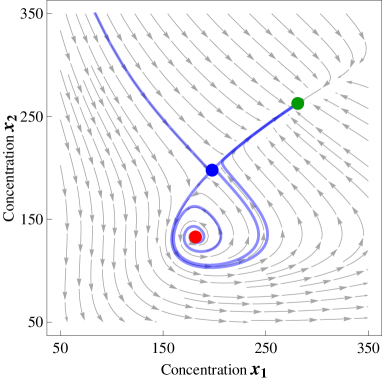
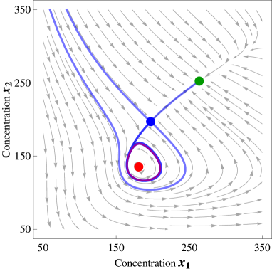
  (a) $\alpha=0.05$                                      (b) $\alpha=-0.05$

     

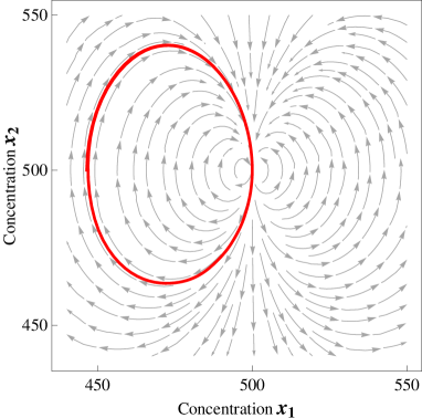
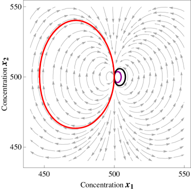
  (c) $\theta=-0.00147$                                (d) $\theta=-0.00145$

Figure 2: (a)–(b) Phase plane diagrams of system $(\ref{eq:homoclinic1})$ before and after the homoclinic bifurcation. The stable node, saddle, and unstable focus are represented as the green, blue and red dots, respectively, the vector field as gray arrows, numerically approximated saddle manifolds as blue trajectories, and the purple curve in panel (b) is the stable limit cycle. The parameters appearing in $(\ref{eq:homoclinic1coefficients})$, and satisfying $(\ref{eq:homoclinic1parameters})$, are fixed to $a=-0.8$, $\mathcal{T}_{1}=\mathcal{T}_{2}=2$, $\varepsilon=0.01$, the reactor volume is set to $V=100$, and the bifurcation parameter $\alpha$ is as shown in the panels. (c)–(d) Phase plane diagrams of system $(\ref{eq:bicyclicXT})$ before and after the multiple limit cycle bifurcation. The stable limit cycles $L_{1}$ and $L_{3}$ are shown in red and purple, respectively, while the unstable limit cycle $L_{2}$ is shown in black. The parameters appearing in $(\ref{eq:bicyclicXT2coefficients})$, and satisfying $(\ref{eq:bicyclicXT2parameters})$, are fixed to $a=1$, $b=-1$, $c=0.5$, $d=0.08$, $x_{1}^{*}=-3$, $\mathcal{T}_{1}=\mathcal{T}_{2}=1000$, $\varepsilon=0.01$, the reactor volume is set to $V=0.5$, and the bifurcation parameter $\theta$ is as shown in the panels.

Consider the following deterministic kinetic equations

$$\frac{\mathrm{d}x_{1}}{\mathrm{d}t} =k_{1}+x_{1}(k_{2}+k_{3}x_{1}-k_{4}x_{2}-k_{5}x_{1}x_{2}+k_{6}x_{2}^{2}),$$

$$\frac{\mathrm{d}x_{2}}{\mathrm{d}t} =k_{7}+x_{2}(-k_{8}+k_{9}x_{1}+k_{10}x_{2}-k_{11}x_{2}^{2}),$$ (9)

with the coefficients $\mathbf{k}=\mathbf{k}(a,\boldsymbol{\mathcal{T}},\alpha,\varepsilon)$ given by

$$k_{1} =\varepsilon,\;\;\;\;\;\;\;\;\;\;\;\;\;\;\;\;\;\;\;\;\;\;\;\;\;\;\;\;\;\;\;\;\;\;\;\;\;\;\;\;\;\;\;\;\;\;\;\;\;\;\;\;\;\;\;\;\;\;\;\;k_{7}=\varepsilon,$$

$$k_{2} =\frac{1}{2}\left|\left(3\left(\mathcal{T}_{2}-\frac{2}{3}\right)(a\mathcal{T}_{1}+\mathcal{T}_{2})-2\alpha\mathcal{T}_{1}\right)\right|,\;\;\;k_{8}=|-\mathcal{T}_{1}+a\mathcal{T}_{2}(\mathcal{T}_{2}-1)|,$$

$$k_{3} =\left|-\frac{3}{2}a\left(\mathcal{T}_{2}-\frac{2}{3}\right)+\alpha\right|,\;\;\;\;\;\;\;\;\;\;\;\;\;\;\;\;\;\;\;\;\;\;\;\;\;\;\;\;k_{9}=1,$$

$$k_{4} =\left|1-\frac{3}{2}(a\mathcal{T}_{1}+2\mathcal{T}_{2})\right|,\;\;\;\;\;\;\;\;\;\;\;\;\;\;\;\;\;\;\;\;\;\;\;\;\;\;\;\;\;\;\;\;k_{10}=\left|2a\left(\mathcal{T}_{2}-\frac{1}{2}\right)\right|,$$

$$k_{5} =\left|\frac{3}{2}a\right|,\;\;\;\;\;\;\;\;\;\;\;\;\;\;\;\;\;\;\;\;\;\;\;\;\;\;\;\;\;\;\;\;\;\;\;\;\;\;\;\;\;\;\;\;\;\;\;\;\;\;\;\;\;\;k_{11}=|a|,$$

$$k_{6} =\frac{3}{2},$$ (10)

where $|\cdot|$ denotes the absolute value, and with parameters $a$, $\alpha$, $\varepsilon$, $\mathcal{T}_{1}$, and $\mathcal{T}_{2}$ satisfying

$$a \in(-1,0),\;\;\;|\alpha|\ll 1,\;\;\;1\ll\varepsilon\leq 0,$$

$$\mathcal{T}_{1} >\frac{2\sqrt{3}}{9},\;\;\;\mathcal{T}_{2}\in\left(\mathrm{max}(1,-a\mathcal{T}_{1}),\frac{2}{3}+\frac{8}{3}a^{-2}(3-a^{2})(a+4\mathcal{T}_{1})\right).$$ (11)

The canonical reaction network [2] induced by system (9) is given by (1).

System (9) is obtained from system [2, eq. (32)], which is known to display a mixed bistability and a convex supercritical homoclinic bifurcation when $\alpha=0$, $\varepsilon=0$. We have modified [2, eq. (32)] by adding to its right-hand side the $\varepsilon$-term from Definition A.1 (i.e. coefficients $k_{1}$ and $k_{7}$ in (9)), thus preventing the long-term dynamics to be trapped on the phase plane axes. It can be shown, using Theorem A.1, that choosing a sufficiently small $\varepsilon>0$ in (10) does not introduce additional positive critical points in the phase space of (9).

In Figures 2(a) and 2(b), we show phase plane diagrams of (9) before and after the bifurcation, respectively, where the critical points of the system are shown as the coloured dots (the stable node, saddle, and unstable focus are shown as the green, blue and red dots, respectively), the blue curves are numerically approximated saddle manifolds (which at $\alpha=0$, $\varepsilon=0$ form a homoclinic loop [2]), and the purple curve in Figure 2(b) is the stable limit cycle that is created from the homoclinic separatrix cycle. Let us note that parameter $\alpha$, appearing in (10), controls the bifurcation, while parameter $a$ controls the saddle-node separation [2].

In Figures 3(a)–(b) and (d)–(e), we show numerical solutions of the initial value problem for (9) in red, with one initial condition in the region of attraction of the node, while the other near the unstable focus. The blue sample paths are generated by using the Gillespie stochastic simulation algorithm on the induced reaction network (1), initiated near the unstable focus. More precisely, in Figures 3(a) and 3(d) we show the dynamics before the deterministic bifurcation, when the node is the globally stable critical point for the deterministic model, while in Figures 3(b) and 3(e) we show the dynamics after the bifurcation, when the deterministic model displays mixed bistability. On the other hand, the stochastic model displays relatively frequent stochastic switching in Figures 3(a) and 3(b), when the saddle-node separation is relatively small. Let us emphasize that the stochastic switching is observed even before the deterministic bifurcation. In Figures 3(d) and 3(e), when the saddle-node separation is relatively large, the stochastic switching is significantly less common, and the stochastic system in the state-space is more likely located near the stable node. Thus, in Figures 3(d) and 3(e), the stochastic system is less affected by the bifurcation than the deterministic system, and, in fact, behaves more like the deterministic system before the bifurcation. This is also confirmed in Figures 3(c) and (f), where we display the $x_{2}$-marginal stationary probability mass functions (PMFs) for the smaller and larger saddle-node separations, respectively, which were obtained by numerically solving the chemical master equation (CME) [42, 43] corresponding to network (1). Let us note that, by sufficiently increasing the saddle-node separation, the left peak in the PMF from Figure 3(f), corresponding to the deterministic limit cycle, becomes nearly zero and difficult to detect.

In [44], we present an algorithm which structurally modifies a given reaction network under mass-action kinetics, in such a way that the deterministic dynamics is preserved, while the stochastic dynamics is modified in a controllable state-dependent manner. We apply the algorithm on reaction network (1), for parameter values similar as in Figures 3(d)–(f), to make the underlying PMF bimodal, so that the underlying sample paths display stochastic switching between the two deterministic attractors. Furthermore, we also make the PMF unimodal, and concentrated around the deterministic limit cycle, so that the underlying sample paths remain near the deterministic limit cycle. Meanwhile, we preserve the deterministic dynamics induced by (9).

      

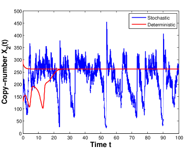
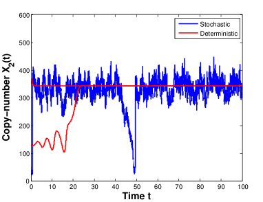
    (a) $a=-0.8$, $\alpha=0.05$                          (d) $a=-0.65$, $\alpha=0.05$

      

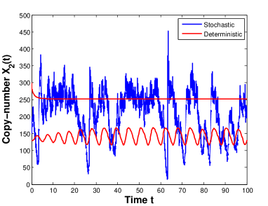
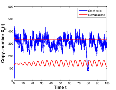
    (b) $a=-0.8$, $\alpha=-0.05$                        (e) $a=-0.65$, $\alpha=-0.05$

      

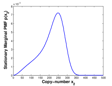
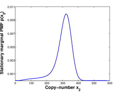
    (c)                                                      (f)

Figure 3: Numerical solutions of system $(\ref{eq:homoclinic1})$ are shown in red. Representative sample paths, generated by the Gillespie stochastic simulation algorithm applied on the corresponding reaction network $(\ref{eq:homoclinic1net})$, are shown in blue. Probability mass functions (PMFs), obtained by numerically solving the underlying chemical master equation (CME) on the bounded domain $(x_{1},x_{2})\in[0,1000]\times[0,600]$, are also shown in blue. (a)–(b) The cases before and after the homoclinic bifurcation, respectively, for smaller values of $a$, when the limit cycle and the stable node are closer together. (d)–(e) The cases before and after the homoclinic bifurcation, respectively, for larger values of $a$. (c) and (f) Stationary $x_{2}$-marginal PMFs. Parameter values in (c) and (f) are the same as in (b) and (e), respectively. One of the deterministic solutions is initiated in the region of attraction of the node, while the other near the focus. The parameters are fixed to $\mathcal{T}_{1}=\mathcal{T}_{2}=2$, $\varepsilon=0.01$, the reactor volume is set to $V=100$, with $a$ and $\alpha$ as shown in the panels.

3.2 System 2: multiple limit cycle bifurcation and bicyclicity

Consider the following deterministic kinetic equations

$$\frac{\mathrm{d}x_{1}}{\mathrm{d}t} =k_{1}+x_{1}(-k_{2}+k_{3}x_{1}+k_{4}x_{2}+k_{5}x_{1}^{2}-k_{6}x_{1}x_{2}-k_{7}x_{2}^{2}),$$

$$\frac{\mathrm{d}x_{2}}{\mathrm{d}t} =k_{8}+x_{2}(k_{9}-k_{10}x_{1}+k_{11}x_{2}+k_{12}x_{1}^{2}-k_{13}x_{1}x_{2}-k_{14}x_{2}^{2}),$$ (12)

with coefficients $\mathbf{k}=\mathbf{k}(a,b,c,d,x_{1}^{*},\boldsymbol{\mathcal{T}},\theta,\varepsilon)$ given by

$$k_{1} =k_{8}=\varepsilon,$$

$$k_{2} =|-a\mathcal{T}_{1}\mathcal{T}_{2}\cos(\theta)+[(d(\mathcal{T}_{1}+1)+c\mathcal{T}_{2})\mathcal{T}_{2}+b(\mathcal{T}_{1}+1)(\mathcal{T}_{1}+x_{1}^{*})]\sin(\theta)|,$$

$$k_{3} =|a\mathcal{T}_{2}\cos(\theta)-[d\mathcal{T}_{2}+b(2\mathcal{T}_{1}+x_{1}^{*}+1)]\sin(\theta)|,$$

$$k_{4} =|a\mathcal{T}_{1}\cos(\theta)-[d(\mathcal{T}_{1}+1)+2c\mathcal{T}_{2}]\sin(\theta)|,$$

$$k_{5} =|b\sin(\theta)|,$$

$$k_{6} =|-a\cos(\theta)+d\sin(\theta)|,$$

$$k_{7} =|c\sin(\theta)|,$$ (13)

and if $k_{i}=|f(a,b,c,d,x_{1}^{*},\boldsymbol{\mathcal{T}})\cos(\theta)-g(a,b,c,d,x_{1}^{*},\boldsymbol{\mathcal{T}})\sin(\theta)|$, then $k_{i+7}=|f(a,b,c,d,x_{1}^{*},\boldsymbol{\mathcal{T}})\sin(\theta)+g(a,b,c,d,x_{1}^{*},\boldsymbol{\mathcal{T}})\cos(\theta)|$, $i=2,3,\ldots,7$, and with parameters $a,$ $b,$ $c,$ $d,$ $x_{1}^{*},$ $\mathcal{T}_{1},$ $\mathcal{T}_{2},$ $\theta$ and $\varepsilon$ satisfying

$$0\leq\varepsilon\ll 1,\,\,\,\,-1\ll\theta<0,$$

$$b<0,\,\,\,\,d>0,\,\,\,\,a>-\frac{d^{2}}{4b},\,\,\,\,0<c<a+\frac{d^{2}}{4b},\,\,\,\,x_{1}^{*}<\frac{d^{2}}{4bc},$$

$$a^{3}c+b^{3}(1-x_{1}^{*})^{2}\neq 0,$$

$$\mathcal{T}_{1}>-x_{1}^{*},\,\,\,\,0<\mathcal{T}_{2}<-\frac{4abx_{1}^{*}}{d^{2}(x_{1}^{*}-1)}(\mathcal{T}_{1}+x_{1}^{*}),$$

$$[d(\mathcal{T}_{1}+1)+c\mathcal{T}_{2}]\mathcal{T}_{2}+b(\mathcal{T}_{1}+1)(\mathcal{T}_{1}+x_{1}^{*})<0.$$ (14)

The canonical reaction network induced by system (12) is given by (3). In this section, we show that systems (12) and (15) (see below), the latter of which is known to display bicyclicity and a multiple limit cycle bifurcation, are topologically equivalent near the corresponding critical points, provided conditions (14) are satisfied.

In Figures 2(c) and 2(d), we show the phase plane diagram of (12) for a particular choice of the parameters satisfying (14), and it can be seen that the system also displays bicyclicity and a multiple limit cycle bifurcation, with Figures 2(c) and 2(d) showing the cases before and after the bifurcation, respectively. In Figure 2(c), the only stable invariant set is the limit cycle shown in red, while in Figure 2(d) there are two additional limit cycles - a stable one, shown in purple, and an unstable one, shown in black. The purple, black and red limit cycles are denoted in the rest of the paper by $L_{1}$, $L_{2}$ and $L_{3}$, respectively. At the bifurcation point, $L_{1}$ and $L_{2}$ intersect.

In order to construct (12), let us consider the planar quadratic ODE system [39, 21] given by

$$\frac{\mathrm{d}x_{1}}{\mathrm{d}t} =\mathcal{Q}_{1}(x_{1},x_{2})\cos(\theta)-\mathcal{Q}_{2}(x_{1},x_{2})\sin(\theta),$$

$$\frac{\mathrm{d}x_{2}}{\mathrm{d}t} =\mathcal{Q}_{1}(x_{1},x_{2})\sin(\theta)+\mathcal{Q}_{2}(x_{1},x_{2})\cos(\theta),$$ (15)

where

$$\mathcal{Q}_{1}(x_{1},x_{2}) =-ax_{1}x_{2},$$

$$\mathcal{Q}_{2}(x_{1},x_{2}) =-bx_{1}^{*}+b(x_{1}^{*}+1)x_{1}+dx_{2}-bx_{1}^{2}-dx_{1}x_{2}-cx_{2}^{2},$$ (16)

with

$$x_{1}^{*} <0,\,\,d^{2}-4bcx_{1}^{*}<0,\,\,d^{2}-4b(c-a)<0,$$

$$\theta d\left(a-b(1-x_{1}^{*})\right) <0,\,\,\,\theta bd>0,\,\,\,a^{3}c+b^{3}(1-x_{1}^{*})^{2}\neq 0.$$ (17)

Lemma 3.1.

Consider system $(\ref{eq:bicyclic})$–$(\ref{eq:bicyclicconditions})$, with the real parameter $\theta\in(-\pi,\pi]$. Function $\boldsymbol{\mathcal{P}}(x_{1},x_{2};\,\theta)=(\mathcal{Q}_{1}\cos(\theta)-\mathcal{Q}_{2}\sin(\theta),\mathcal{Q}_{1}\sin(\theta)+\mathcal{Q}_{2}\cos(\theta))$ forms a one-parameter family of uniformly rotated vector fields with the rotation parameter $\theta$, and the following results hold:

1. Finite critical points. System $(\ref{eq:bicyclic})$ has two critical points in the finite part of the phase plane, located at $(1,0)$ and $(x_{1}^{*},0)$, both of which are unstable foci when $|\theta|\ll 1$.

2. Number and distribution of limit cycles. System $(\ref{eq:bicyclic})$ has three limit cycles in the configuration $(2,1)$ when $|\theta|\ll 1$. The focus located at $(1,0)$ is surrounded by two positively oriented limit cycles $L_{1}$ and $L_{2}$, with the unstable limit cycle $L_{2}$ enclosing the stable limit cycle $L_{1}$, while the focus at $(x_{1}^{*},0)$ by a single negatively oriented stable limit cycle $L_{3}$.

3. Dependence of the limit cycles on the rotation parameter $\theta$. There exists a critical value $\theta=\theta^{*}<0$, at which the limit cycles $L_{1}$ and $L_{2}$ intersect in a semistable, positively oriented limit cycle that is stable from the inside, and unstable from the outside. As $\theta$ is monotonically increased in $(\theta^{*},0)$, the limit cycles $L_{2}$ and $L_{3}$ monotonically expand, while $L_{1}$ monotonically contracts.

Proof.

The statement of the lemma follows from [39, 21], and the theory of one-parameter family of uniformly rotated vector fields [40, 22]. ∎

In order to map the stable limit cycles of system (15) into the first quadrant, and then map the resulting system to a kinetic one, having no boundary critical points, let us apply a translation transformation $\Psi_{\mathcal{T}}$ [2], $\boldsymbol{\mathcal{T}}=(\mathcal{T}_{1},\mathcal{T}_{2})\in\mathbb{R}^{2}$, followed by a perturbed $x$-factorable transformation, as defined in Definition A.1, on system (15), which results in system (12) with the coefficients (13).

Theorem 3.1.

Consider the ODE systems $(\ref{eq:bicyclicXT})$ and $(\ref{eq:bicyclic})$, and assume conditions $(\ref{eq:bicyclicXT2parameters})$ are satisfied. Then $(\ref{eq:bicyclicXT})$ and $(\ref{eq:bicyclic})$ are locally topologically equivalent in the neighborhood of the corresponding critical points. Furthermore, for sufficiently small $\varepsilon>0$, system $(\ref{eq:bicyclicXT})$ has exactly one additional critical point in $\mathbb{R}_{>}^{2}$, which is a saddle located in the neigbhourhood of $(\mathcal{T}_{1},0)$.

Proof.

Consider the critical point $(1,0)$ of system (15), which corresponds to the critical point $(\mathcal{T}_{1}+1,\mathcal{T}_{2})$ of system (12) when $\varepsilon=0$. The Jacobian matrices of (15), and (12) with $\varepsilon=0$, evaluated at $(1,0)$, and $(\mathcal{T}_{1}+1,\mathcal{T}_{2})$, are respectively given by

$$J =\left(\begin{array}[]{cc}-b(x_{1}^{*}-1)\sin(\theta)&\;\;-a\cos(\theta)\\ b(x_{1}^{*}-1)\cos(\theta)&\;\;-a\sin(\theta)\end{array}\right),$$ (20)

$$J_{\mathcal{X},\mathcal{T}} =\left(\begin{array}[]{cc}-b(x_{1}^{*}-1)(\mathcal{T}_{1}+1)\sin(\theta)&\;\;-a(\mathcal{T}_{1}+1)\cos(\theta)\\ b(x_{1}^{*}-1)\mathcal{T}_{2}\cos(\theta)&\;\;-a\mathcal{T}_{2}\sin(\theta)\end{array}\right).$$ (23)

Condition (ii) of [2, Theorem 3.3] is satisfied, so that the stability of the critical point is preserved under the $x$-factorable transformation, but condition (iii) is not satisfied. In order for $(\mathcal{T}_{1}+1,\mathcal{T}_{2})$ to remain focus under the $x$-factorable transformation, the discriminant of $J_{\mathcal{X},\mathcal{T}}$ must be negative:

$$(a\mathcal{T}_{2}+b(\mathcal{T}_{1}+1)(x_{1}^{*}-1))^{2}(\sin(\theta))^{2}-4ab(x_{1}^{*}-1)(\mathcal{T}_{1}+1)\mathcal{T}_{2} <0.$$ (24)

Let us set $\theta=0$ in (24), leading to

$$-4ab(x_{1}^{*}-1)(\mathcal{T}_{1}+1)\mathcal{T}_{2} <0.$$ (25)

Conditions (24) and (25) are equivalent when $|\theta|\ll 1$, since the the sign of the function on the LHS of (24) is a continuous function of $\theta$. From conditions (14) it follows that $ab<0$, $x_{1}^{*}<0$, and $\mathcal{T}_{1},\mathcal{T}_{2}>0$, so that (25) is satisfied. Similar arguments show that the second critical point of (15), located at $(x_{1}^{*},0)$, is mapped to an unstable focus of (12), if $d>0$, and if $\mathcal{T}_{2}$ is bounded as given in (14).

Consider (12) with $\varepsilon=0$. The boundary critical points are located at $(0,0)$, $(\mathcal{T}_{1},0)$, and $(0,x_{2,\pm}^{*})$, with

$$x_{2,\pm}^{*} =\frac{1}{2c}\left(d(\mathcal{T}_{1}+1)+2c\mathcal{T}_{2}\pm\sqrt{(\mathcal{T}_{1}+1)(d^{2}(\mathcal{T}_{1}+1)-4bc(\mathcal{T}_{1}+x_{1}^{*}))}\right).$$

Conditions (14) imply that the critical point $(0,0)$ satisfies $\mathcal{P}_{1}(0,0)=-a\mathcal{T}_{1}\mathcal{T}_{2}<0$, and

$$\mathcal{P}_{2}(0,0) =-[d(1+\mathcal{T}_{1})+c\mathcal{T}_{2}]\mathcal{T}_{2}-b(1+\mathcal{T}_{1})(\mathcal{T}_{1}+x_{1}^{*})>0,$$

when $\theta=0$. When $|\theta|\ll 1$, it then follows from condition (iv) of [2, Theorem 3.3] that the critical point is a saddle, and from Theorem A.1, condition (29), that it is mapped outside of $\mathbb{R}_{\geq}^{2}$ when $\varepsilon\neq 0$. Similar arguments show that, assuming conditions (14) are true, $(\mathcal{T}_{1},0)$ is a saddle that is mapped to $\mathbb{R}_{>}^{2}$ when $\varepsilon\neq 0$, and that critical points $(0,x_{2,\pm}^{*})$ are real, $x_{2,-}^{*}<0$, and that $(0,x_{2,+}^{*})$ is a saddle that is mapped outside $\mathbb{R}_{\geq}^{2}$ when $\varepsilon\neq 0$.

Finally, if conditions (14) are satisfied, so are conditions (17). ∎

We now consider the kinetic ODEs (12) and the induced reaction network (4) for a particular set of coefficients (13). We also rescale the time according to $t\to 2\times 10^{-5}\,t$, i.e. we multiply all the coefficients $k_{1},\ldots k_{14}$ appearing in (12) by $2\times 10^{-5}$. On this time-scale, we capture dynamical effects relevant for this paper. In Figures 4(a) and 4(b) we show numerically approximated solutions of the initial value problem for (12) before and after the bifurcation, respectively. In Figure 4(a), the solution is initiated near the unstable focus outside the limit cycle $L_{3}$, and it can be seen that the solution spends some time near the unstable focus, followed by an excursion that leads it to the stable limit cycle $L_{3}$, where is then stays forever. In Figure 4(b), the solutions tend to the limit cycle $L_{1}$ or $L_{3}$, depending on the initial condition. Let us note that the critical value at which the limit cycles $L_{1}$ and $L_{2}$ intersect, at the deterministic level, is numerically found to be $\theta^{*}\approx-0.00146$.

In Figures 4(c) and 4(d) we show representative sample paths generated by applying the Gillespie stochastic simulation algorithm on the reaction network (3), before and after the bifurcation, respectively. One can notice that the stochastic dynamics does not appear to be significantly influenced by the bifurcation, as opposed to the deterministic dynamics. In Figures 4(c) and 4(d), one can notice pulses similar as in Figure 4(a), that are now induced by the intrinsic noise present in the system.

The stationary PMF corresponding to network (3), for parameter values as in Figures 4(c) and 4(d), accumulates at the boundary of the state-space (see also the Keizer paradox [45]). While the results from Appendix A may be used to prevent a PMF from accumulating at the boundary, one may need a sufficiently large reactor volume. For example, for network (1), the propensity function [43] of reactions $r_{1}$ and $r_{7}$, for parameter values taken in this paper (i.e. $\varepsilon=0.01$ in (10), and $V=100$), takes the value $\varepsilon V=1$. This is sufficient for the underlying PMF to approximately vanish at the boundary of the state-space, as demonstrated in Figures 3(c) and (f). On the other hand, for network (3), we take $\varepsilon=0.01$ in (13), and $V=0.5$, so that the propensity function of $r_{1}$ and $r_{8}$ takes the value of only $0.005$. As a consequence, the underlying PMF accumulates at the boundary of the state-space. Instead of increasing the reactor volume to prevent this, we instead focus on the so-called quasi-stationary PMF under the condition that the species copy-numbers are positive, $p_{>}(x,y)\equiv p(x,y|x>0,y>0)$. The quasi-stationary PMF describes well the stochastic dynamics of network (3) on the time-scale of interest, presented in Figures 4(c) and 4(d). In Figure 4(e), we display an approximate $x_{1}$-marginal quasi-stationary PMF $p_{>}(x_{1})$, for the same parameter values as in Figure 4(d). The quasi-stationary PMF $p_{>}(x_{1})$ was obtained by numerically solving the stationary CME corresponding to network (3), on a truncated domain which excludes the boundary of the state-space.

      

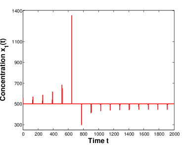
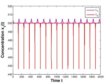
    (a) $\theta=-0.00147$                                  (b) $\theta=-0.00145$

      

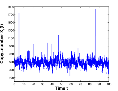
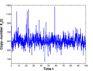
    (c) $\theta=-0.00147$                                  (d) $\theta=-0.00145$

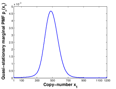
                       (e)

Figure 4: (a)–(b) Numerical solutions of the kinetic ODE system given by $(\ref{eq:bicyclicXT})$ before and after the bifurcation, where in (b) the trajectory initiated near the stable limit cycle $L_{1}$ is shown in purple, while the one initiated near $L_{3}$ in red. (c)–(d) Sample paths generated by the Gillespie stochastic simulation algorithm applied to the induced reaction network $(\ref{eq:bicyclicXT2net})$ before and after the bifuration. (e) Approximate quasi-stationary $x_{1}$-marginal PMF, obtained by numerically solving the stationary CME, corresponding to network (3), on the bounded domain $(x_{1},x_{2})\in[1,1200]\times[1,1200]$, for the same parameters values as in (d). The parameters appearing in $(\ref{eq:bicyclicXT2coefficients})$ are fixed to $a=1$, $b=-1$, $c=0.5$, $d=0.08$, $x_{1}^{*}=-3$, $\mathcal{T}_{1}=\mathcal{T}_{2}=1000$, $\varepsilon=0.01$, with the reactor volume $V=0.5$, and $\theta$ as indicated in the plots. Coefficients $(\ref{eq:bicyclicXT2coefficients})$ are multiplied by a constant factor of $2\times 10^{-5}$ (time-rescaling).

4 Summary

In the first part of the paper, in Section 2, we have presented theoretical results regarding oscillations, oscillation-related bifurcations and multistability in the planar quadratic kinetic ODEs (6), which are (appropriately) bounded in the nonnegative quadrant. Such ODEs are used in applications to describe the deterministic dynamics of concentrations of two biological/chemical species, with at most quadratic interactions. While the kinetic ODEs (6) inherit many properties from the more general planar quadratic ODEs (5), some properties, which are of biological/chemical relevance, are not necessarily inherited. For example, we have formulated the following open problem: while general planar quadratic ODEs (5) may display bicyclicity (a coexistence of two stable oscillatory attractors), is the same true for the kinetic planar quadratic ODEs (6)?

In Section 3, building upon the results from Section 2, and using the results from [2] and Appendix A, we have constructed two reaction networks, with the deterministic dynamics described by planar cubic kinetic ODEs. The first network is given by (1), and, at the deterministic level, displays a homoclinic bifurcation, and a coexistence of a stable critical point and a stable limit cycle (mixed bistability). The second network is given by (3), and, at the deterministic level, displays a multiple limit cycle bifurcation, and a coexistence of two stable limit cycles (bicyclicity). The phase planes of the kinetic ODEs induced by the first network before and after the bifurcation are shown in Figures 2(a) and 2(b), respectively, while for the second network in Figures 2(c) and 2(d).

In Figure 3, we have compared the deterministic and stochastic solutions corresponding to the first reaction network (1), with the rate coefficients such that the deterministic solutions are close to the homoclinic bifurcation. Analogously, in Figure 4, we have done the same for reaction network (3), when the deterministic solutions are close to the multiple limit cycle bifurcation. In both Figures 3 and 4, we observe qualitative differences between the deterministic and stochastic dynamics. In particular, the stochastic dynamics in Figure 3 may display stochastic switching near the deterministic bifurcation. Furthermore, the dynamics of both networks are not affected qualitatively by the deterministic bifurcation sharply at the bifurcation point.

In Section 1, we have outlined the statistical inference problem, consisting of detecting and classifying cycles (oscillations) in noisy time-series, and we have put forward networks (1) and (3) as suitable test problems. Network (1) poses two inference challenges: firstly, let us consider the scenario shown in Figures 3(d)–(f). In this case, the relative separation between the two deterministic attractors is larger. Consequently, at the stochastic level, the corresponding marginal probability mass function (PMF), shown in Figure 3 (f), is bimodal. However, the left peak, corresponding to the deterministic limit cycle, is much smaller than the right peak, corresponding to the deterministic critical point (a node). Using the shape of the marginal PMF, as put forward in [1], one cannot conclude the presence of a noisy limit cycle. Let us note that, by sufficiently increasing the distance between the two attractors, the left PMF peak from Figure 3(f) approximately vanishes, making the inference problem even harder. On the other hand, using the covariance function (and spectral analysis), as put forward in [1], may also be limited, as the noisy time-series spends a smaller amount of time near the deterministic limit cycle, as demonstrated in Figure 3(e). Secondly, let us consider the scenario shown in Figures 3(a)–(c), when the relative separation between the two deterministic attractors is smaller. In this case, it may be a challenge to infer that there are two distinct attractors ‘hidden’ in the time-series shown in Figure 3(b), and the PMF shown in Figure 3(c). The fact that the PMF in Figure 3(c) is a non-Gaussian may be used as an indication of a certain dynamical complexity. The problem becomes more difficult for network (3), with two stable deterministic limit cycles ‘hidden’ in the noisy time-series shown in Figure 4(d), and in the PMF shown in Figure 4(e). Let us note that the PMF is approximately Gaussian, and this persists for a wide range of larger reactor volumes.

Acknowledgments: The authors would like to thank the Isaac Newton Institute for Mathematical Sciences, Cambridge, for support and hospitality during the programme “Stochastic Dynamical Systems in Biology: Numerical Methods and Applications” where work on this paper was undertaken. This work was supported by EPSRC grant no EP/K032208/1. This work was partially supported by a grant from the Simons Foundation. Tomáš Vejchodský would like to acknowledge the institutional support RVO 67985840. Radek Erban would also like to thank the Royal Society for a University Research Fellowship.

Appendix A : perturbed $x$-factorable transformation

Definition A.1.

Consider applying an $x$-factorable transformation, as defined in [2], on (5), and then adding to the resulting right-hand side a zero-degree term $\varepsilon\mathbf{v}$, with $\varepsilon\geq 0$ and vector $\mathbf{v}=(1,1)^{\top}$, resulting in

$$\frac{\mathrm{d}\mathbf{x}}{\mathrm{d}t} =\varepsilon\mathbf{v}+\mathcal{X}(\mathbf{x})\boldsymbol{\mathcal{P}}(\mathbf{x};\,\mathbf{k})\,=\,\varepsilon\mathbf{v}+(\Psi_{\mathcal{X}}\boldsymbol{\mathcal{P}})(\mathbf{x};\,\mathbf{k})\equiv(\Psi_{\mathcal{X}_{\varepsilon}}\boldsymbol{\mathcal{P}})(\mathbf{x};\,\mathbf{k}).$$ (26)

Then $\Psi_{\mathcal{\mathcal{X}_{\varepsilon}}}:\mathbb{P}_{2}(\mathbb{R}^{2};\,\mathbb{R}^{2})\to\mathbb{P}_{3}(\mathbb{R}^{2};\,\mathbb{R}^{2})$, mapping $\boldsymbol{\mathcal{P}}(\mathbf{x};\,\mathbf{k})$ to $(\Psi_{\mathcal{X}_{\varepsilon}}\boldsymbol{\mathcal{P}})(\mathbf{x};\,\mathbf{k})$, is called a perturbed $x$-factorable transformation if $\varepsilon\neq 0$. If $\varepsilon=0$, the transformation reduces to an (unperturbed) $x$-factorable transformation, $\Psi_{\mathcal{\mathcal{X}}}\equiv\Psi_{\mathcal{X}_{0}}$, defined in [2].

Lemma A.1.

$(\Psi_{\mathcal{X}_{\varepsilon}}\boldsymbol{\mathcal{P}})(\mathbf{x};\,\mathbf{k})$ from Defnition A.1 is a kinetic function, i.e. $(\Psi_{\mathcal{X}_{\varepsilon}}\boldsymbol{\mathcal{P}})(\mathbf{x};\,\mathbf{k})\in\mathbb{P}^{\mathcal{K}}_{3}(\mathbb{R}_{\geq}^{2};\,\mathbb{R}^{2})$.

Proof. $(\Psi_{\mathcal{X}}\boldsymbol{\mathcal{P}})(\mathbf{x};\,\mathbf{k})$ is a kinetic function [2]. Since, from (26), $(\Psi_{\mathcal{X}_{\varepsilon}}\boldsymbol{\mathcal{P}})(\mathbf{x};\,\mathbf{k})=\varepsilon\mathbf{v}+(\Psi_{\mathcal{X}}\boldsymbol{\mathcal{P}})(\mathbf{x};\,\mathbf{k})$, with $\varepsilon\geq 0$ and $\mathbf{v}=(1,1)^{\top}$, it follows that $(\Psi_{\mathcal{X}_{\varepsilon}}\boldsymbol{\mathcal{P}})(\mathbf{x};\,\mathbf{k})$ is kinetic as well. ∎

We now provide a theorem relating location, stability and type of the positive critical points of (5) and (26).

Theorem A.1.

Consider the ODE system $(\ref{eq:polynomial})$ with positive critical points $\mathbf{x}^{*}\in\mathbb{R}_{>}^{2}$. Let us assume that $\mathbf{x}^{*}\in\mathbb{R}_{>}^{2}$ is hyperbolic, and is not the degenerate case between a node and a focus, i.e. it satisfies the condition

$$\left(\textrm{\emph{tr}}\left(\nabla\boldsymbol{\mathcal{P}}(\mathbf{x}^{*};\,\mathbf{k})\right)\right)^{2}-4\textrm{\emph{det}}\left(\nabla\boldsymbol{\mathcal{P}}(\mathbf{x}^{*};\,\mathbf{k})\right) \neq 0,$$ (27)

as well as conditions (ii) and (iii) of Theorem $3.3$ in [2]. Then positivity, stability and type of the critical point $\mathbf{x}^{*}\in\mathbb{R}_{>}^{2}$ are invariant under the perturbed $x$-factorable transformations $\Psi_{\mathcal{X}_{\varepsilon}}$, for sufficiently small $\varepsilon\geq 0$. Assume $(\ref{eq:polynomial})$ does not have boundary critical points. Consider the two-dimensional ODE system $(\ref{eqn:xft})$ with $\varepsilon=0$, and with boundary critical points denoted $\mathbf{\bar{x}}^{0}\in\mathbb{R}_{\geq}^{2}$, $\mathbf{\bar{x}}^{0}=(\bar{x}_{b,1}^{0},\bar{x}_{b,2}^{0})$, $\bar{x}_{b,1}^{0}\bar{x}_{b,2}^{0}=0$. Assume that for $i\in\{1,2\}$

$$\frac{\partial\mathcal{P}_{i}(\mathbf{\bar{x}}_{b}^{0};\,\mathbf{k})}{\partial x_{i}} \neq 0,\,\,\,\,\,\,\,\,\,\text{if }\,\,\,\bar{x}_{b,i}^{0}\,\neq\,0,$$ (28)

and that for some $i\in\{1,2\}$

$$\mathcal{P}_{i}(\mathbf{\bar{x}}_{b}^{0};\,\mathbf{k}) >0,\,\,\,\,\,\,\,\,\,\text{if }\,\,\,\bar{x}_{b,i}^{0}\,=\,0.$$ (29)

Then, the critical point $\mathbf{\bar{x}}_{b}^{0}\in\mathbb{R}_{\geq}^{2}$ of the two-dimensional ODE system $(\ref{eqn:xft})$ with $\varepsilon=0$ becomes the critical point $\mathbf{\bar{x}}_{b}\notin\mathbb{R}_{\geq}^{2}$ of system $(\ref{eqn:xft})$ for sufficiently small $\varepsilon>0$.

Proof.

The critical points of (26) are solutions of the following regularly perturbed algebraic equation

$$\varepsilon\mathbf{v}+\mathcal{X}(\mathbf{\bar{x}})\boldsymbol{\mathcal{P}}(\mathbf{\bar{x}};\,\mathbf{k}) =\mathbf{0}.$$ (30)

Let us assume $\mathbf{\bar{x}}$ can be written as the power series

$$\mathbf{\bar{x}} =\mathbf{\bar{x}}^{0}+\varepsilon\mathbf{\bar{x}}^{1}+\mathcal{O}(\varepsilon^{2}),$$ (31)

where $\mathbf{\bar{x}}^{0}\in\mathbb{R}_{\geq}^{2}$ are the critical points of (26) with $\varepsilon=0$. Substituting the power series (31) into (30), and using the Taylor series theorem on $\boldsymbol{\mathcal{P}}(\mathbf{\bar{x}};\,\mathbf{k})$, so that $\boldsymbol{\mathcal{P}}(\mathbf{\bar{x}}^{0}+\varepsilon\mathbf{\bar{x}}^{1}+\mathcal{O}(\varepsilon^{2});\,\mathbf{k})=\boldsymbol{\mathcal{P}}(\mathbf{\bar{x}}^{0};\,\mathbf{k})+\varepsilon\nabla\boldsymbol{\mathcal{P}}(\mathbf{\bar{x}}^{0};\,\mathbf{k})\mathbf{\bar{x}}^{1}+\mathcal{O}(\varepsilon^{2})$, as well as that $\mathcal{X}(\mathbf{\bar{x}})=\mathcal{X}(\mathbf{\bar{x}}^{0})+\varepsilon\mathcal{X}(\mathbf{\bar{x}}^{1})+\mathcal{O}(\varepsilon^{2})$, and equating terms of equal powers in $\varepsilon$, the following system of polynomial equations is obtained:

$$\mathcal{O}\left(1\right): \;\mathcal{X}(\mathbf{\bar{x}}^{0})\boldsymbol{\mathcal{P}}(\mathbf{\bar{x}}^{0};\,\mathbf{k})\,=0,$$

$$\mathcal{O}(\varepsilon): \;\mathcal{X}(\mathbf{\bar{x}}^{0})\nabla\boldsymbol{\mathcal{P}}(\mathbf{\bar{x}}^{0};\,\mathbf{k})\mathbf{\bar{x}}^{1}+\mathcal{X}(\mathbf{\bar{x}}^{1})\boldsymbol{\mathcal{P}}(\mathbf{\bar{x}}^{0};\,\mathbf{k})\,=-\mathbf{v}.$$ (32)

Order $1$ equation. The positive critical points $\mathbf{\bar{x}}^{0}\in\mathbb{R}_{>}^{2}$ satisfy $\boldsymbol{\mathcal{P}}(\mathbf{\bar{x}}^{0};\,\mathbf{k})=\mathbf{0}$. Since $\boldsymbol{\mathcal{P}}(\mathbf{x};\,\mathbf{k})$ has no boundary critical points by assumption, critical points $\mathbf{\bar{x}}_{b}^{0}\in\mathbb{R}_{\geq}^{2}$ with $\bar{x}_{b,i}^{0}=0$, $\bar{x}_{b,j}^{0}\neq 0$, $\bar{x}_{b,1}^{0}\bar{x}_{b,2}^{0}=0$, $i,j\in\{1,2\}$, satisfy $\mathcal{P}_{i}(\mathbf{\bar{x}}_{b}^{0};\,\mathbf{k})\neq 0$, $\mathcal{P}_{j}(\mathbf{\bar{x}}_{b}^{0};\,\mathbf{k})=0$.

Order $\varepsilon$ equation. Vector $\mathbf{\bar{x}}^{1}$, corresponding to a positive $\mathbf{\bar{x}}^{0}$, satisfies

$$\mathcal{X}(\mathbf{\bar{x}}^{0})\nabla\boldsymbol{\mathcal{P}}(\mathbf{\bar{x}}^{0};\,\mathbf{k})\mathbf{\bar{x}}^{1} =-\mathbf{v},$$

which can be solved provided $\mathbf{\bar{x}}^{0}$ is a hyperbolic critical point. Vector $\mathbf{\bar{x}}_{b}^{1}$, corresponding to a nonnegative $\mathbf{\bar{x}}_{b}^{0}$, is given by

$$\bar{x}_{b,i}^{1}=\begin{cases}-(\mathcal{P}_{i}(\mathbf{\bar{x}}_{b}^{0};\,\mathbf{k}))^{-1},&\textrm{if }\bar{x}_{b,i}^{0}=0,\\ (\frac{\partial\mathcal{P}_{i}(\mathbf{\bar{x}}_{b}^{0};\,\mathbf{k})}{\partial x_{i}})^{-1}\left((\mathcal{P}_{j}(\mathbf{\bar{x}}_{b}^{0};\,\mathbf{k}))^{-1}\frac{\partial\mathcal{P}_{i}(\mathbf{\bar{x}}_{b}^{0};\,\mathbf{k})}{\partial x_{j}}-(\bar{x}_{b,i}^{0})^{-1}\right),&\textrm{if }\bar{x}_{b,i}^{0}\neq 0,\end{cases}$$

from which conditions (28) and (29) follow. ∎

Appendix B : bicyclic system with large attractors

Consider the following deterministic kinetic equations

$$\frac{\mathrm{d}x_{1}}{\mathrm{d}t} =k_{1}+x_{1}(-k_{2}+k_{3}x_{1}+k_{4}x_{2}-k_{5}x_{1}x_{2}),$$

$$\frac{\mathrm{d}x_{2}}{\mathrm{d}t} =k_{6}+x_{2}(k_{7}-k_{8}x_{1}+k_{9}x_{2}+k_{10}x_{1}^{2}-k_{11}x_{2}^{2}),$$ (33)

with the coefficients $\mathbf{k}$ given by

$$k_{1} =10^{-3},\;\;\;k_{2}=10,\;\;\;k_{3}=1,\;\;\;k_{4}=1,\;\;\;k_{5}=0.1,\;\;\;k_{6}=10^{-3},$$

$$k_{7} =3.7,\;\;\;k_{8}=1.9,\;\;\;k_{9}=1.01,\;\;\;k_{10}=0.1,\;\;\;k_{11}=0.05.$$ (34)

The canonical reaction network induced by system (33), involving two species $s_{1}$ and $s_{2}$ and eleven reactions $r_{1},r_{2},\ldots,r_{11}$ under mass-action kinetics, is given by

$$r_{1}:\; \varnothing \xrightarrow[]{k_{1}}s_{1},\;\;\;\;\;\;\;\;\;\;\;\;\;\;\;\;\;\;\;\;\;\;\;\;\;\;\;\;\;\;\;\;\;\;\,r_{6}: \varnothing \xrightarrow[]{k_{6}}s_{2},$$

$$r_{2}:\; s_{1} \xrightarrow[]{k_{2}}\varnothing,\;\;\;\;\;\;\;\;\;\;\;\;\;\;\;\;\;\;\;\;\;\;\;\;\;\;\;\;\;\;\;\;\;\;\,\,r_{7}: s_{2} \xrightarrow[]{k_{7}}2s_{2},$$

$$r_{3}:\; 2s_{1} \xrightarrow[]{k_{3}}3s_{1},\;\;\;\;\;\;\;\;\;\;\;\;\;\;\;\;\;\;\;\;\;\;\;\;\;\;\;\;\;\;\;\;\,r_{8}: s_{1}+s_{2} \xrightarrow[]{k_{8}}s_{1},$$

$$r_{4}:\; s_{1}+s_{2} \xrightarrow[]{k_{4}}2s_{1}+s_{2},\;\;\;\;\;\;\;\;\;\;\;\;\;\;\;\;\;\;\;\;\;\;\;\;\;r_{9}: 2s_{2} \xrightarrow[]{k_{9}}3s_{2},$$

$$r_{5}:\; 2s_{1}+s_{2} \xrightarrow[]{k_{5}}s_{1}+s_{2},\;\;\;\;\;\;\;\;\;\;\;\;\;\;\;\;\;\;\;\;\;\;\;\;\;\,r_{10}: 2s_{1}+s_{2} \xrightarrow[]{k_{10}}2s_{1}+2s_{2},$$

$$\;\;\;\;\;\;\;\;\;\;\;\;\;\;\;\;\;\;\;\;\;\;\;\;\;\;\;\;\;\;\;\;\;\;\;\;\;\;\;\;\;\;\;\;\;r_{11}: 3s_{2} \xrightarrow[]{k_{11}}2s_{2}.$$ (35)

In Figure (5)(a), we show the two stable limit cycles obtained by numerically solving (33) with parameters (34). In Figure (5)(b), in addition to the limit cycles, we also show in blue a representative sample path obtained by applying the Gillespie algorithm on (35). Let us note that (33) was constructed in a similar fashion as system (12) in Section 3.2, using the results from [46, 39].

 

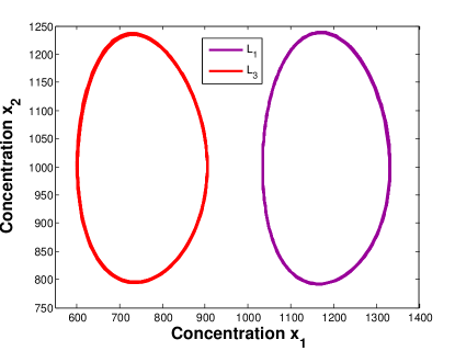
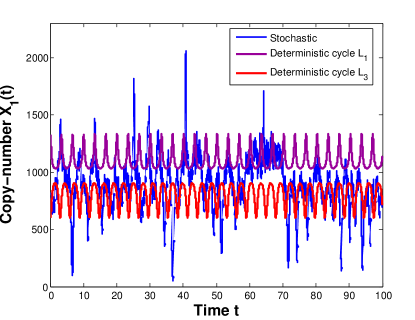
(a)                                                    (b)

Figure 5: Panel (a) displays numerically approximated stable limit cycles $L_{1}$ and $L_{3}$ in the state-space of system $(\ref{eq:bicyclicXT2})$, with parameters $(\ref{eq:bicyclicexample2})$ and reactor volume $V=100$. Panel (b) displays in blue a representative sample path, generated by applying the Gillespie algorithm on the underlying reaction network $(\ref{eq:bicyclicXT2net2})$ for the same parameters as in panel (a). Also shown are two deterministic trajectories, one initiated near the limit cycle $L_{1}$, while the other near $L_{3}$. One can observe that the stochastic sample path switches between the two deterministic attractors.

References

- [1] Pineda-Krch, M., Blok, H. J., Dieckmann, U., Doebeli, M., 2007. A tale of two cycles – distinguishing quasi-cycles and limit cycles in finite predator-prey populations. Oikos, 116(1): 53–64.
- [2] Plesa, T., Vejchodský, T., and Erban, R., 2016. Chemical Reaction Systems with a Homoclinic Bifurcation: An Inverse Problem. Journal of Mathematical Chemistry, 54(10): 1884–1915.
- [3] Érdi, P., Tóth, J. Mathematical Models of Chemical Reactions. Theory and Applications of Deterministic and Stochastic Models. Manchester University Press, Princeton University Press, 1989.
- [4] Toner, D. L. K., Grima R., 2013. Molecular noise induces concentration oscillations in chemical systems with stable node steady states. The Journal of Chemical Physics, 138, 055101.
- [5] Louca, S., Doebeli, M., 2014. Distinguishing intrinsic limit cycles from forced oscillations in ecological time series. Theoretical Ecology, 7(4): 381–390.
- [6] Erban, R., Chapman, S. J., Kevrekidis, I. and Vejchodský, T., 2009. Analysis of a stochastic chemical system close to a SNIPER bifurcation of its mean-field model. SIAM Journal on Applied Mathematics, 70(3): 984–1016.
- [7] Liao, S., Vejchodský, T., and Erban, R., 2015. Tensor methods for parameter estimation and bifurcation analysis of stochastic reaction networks. Journal of The Royal Society Interface, 12(108), 20150233.
- [8] Thomas, P., Straube, A. V., Timmer, J., Fleck, C., Grima R., 2013. Signatures of nonlinearity in single cell noise-induced oscillations. Journal of Theoretical Biology, 335: 222–234.
- [9] Vance, W., Ross, J., 1996. Fluctuations near limit cycles in chemical reaction systems. The Journal of Chemical Physics, 105: 479–487.
- [10] Boland, R. P., Galla, T., McKane, A. J., 2008. How limit cycles and quasi-cycles are related in systems with intrinsic noise. Journal of Statistical Mechanics: Theory and Experiment, P09001.
- [11] Xiao, T., Ma, J., Hou, Z., Xin, H., 2007. Effects of internal noise in mesoscopic chemical systems near Hopf bifurcation. New Journal of Physics, 9, 403.
- [12] Borisuk, M. T., Tyson, J. J., 1998. Bifurcation Analysis of a Model of Mitotic Control in Frog Eggs. Journal of Theoretical Biology, 195: 69–85.
- [13] Li, M. Y., and Shu, H., 2011. Multiple Stable Periodic Oscillations in a Mathematical Model of CTL Response to HTLV-I Infection. Bulletin of Mathematical Biology, 73: 1774–1793.
- [14] Amiranashvili, A., Schnellbächer, N. D., and Schwarz, U. S., 2016. Stochastic switching between multistable oscillation patterns of the Min-system. New Journal of Physics, 18: 093049.
- [15] Schlögl , F., 1972. Chemical reaction models for nonequilibrium phase transition. Z. Physik., 253(2): 147–161.
- [16] Gaiko, V. A. Global Bifurcation Theory and Hilbert’s Sixteenth Problem. Springer Science, 2003.
- [17] Gaiko, V. A., 2009. On the Geometry of Polynomial Dynamical Systems. Journal of Mathematical Sciences, 157(3): 400–412.
- [18] Perko, L. M., 1984. Limit Cycles of Quadratic Systems in the Plane. Rocky Mountain Journal of Mathematics, 14(3): 619–645.
- [19] Cherkas, L. A., Artés, J. C., Llibre, J., 2003. Quadratic Systems with Limit Cycles of Normal Size. Buletinul Academiei de Ştiinţe a Republicii Moldova. Matematica, 1(41): 31–46.
- [20] Artés, J. C., Llibre, J., 1997. Quadratic Vector Fields with a Weak Focus of Third Order. Publicacions Mathemàtiques, 41: 7–39.
- [21] Escher, C., 1981. Bifurcation and Coexistence of Several Limit Cycles in Models of Open Two-Variable Quadratic Mass-Action Systems. Chemical Physics, 63: 337–348.
- [22] Perko, L. M. Differential Equations and Dynamical Systems, Third Edition. Springer-Verlag, New York, 2001.
- [23] Dutt, A. K., 1992. Asymptotically Stable Limit Cycles in a Model of Glycolytic Oscillations. Chemical Physics Letters, 208: 139–142.
- [24] Kar, S., Baumann, W. T., Pau,l M. R. and Tyson, J. J., 2009. Exploring the Roles of Noise in the Eukaryotic Cell Cycle. Proceedings of the National Academy of Sciences of USA, 106: 6471–6476.
- [25] Vilar, J. M. G., Kueh, H. Y., Barkai, N. and Leibler, S., 2002. Mechanisms of Noise-resistance in Genetic Oscillators. Proceedings of the National Academy of Sciences of the United States of America, 99(9): 5988–5992.
- [26] Kuznetsov, Y. A. Elements of Applied Bifurcation Theory, Second Edition. Springer-Verlag, New York, 2000.
- [27] Ghomi, M. S., Ciliberto, A., Kar, S., Novak, B., Tyson, J. J., 2008. Antagonism and Bistability in Protein Interaction Networks. Journal of Theoretical Biology, 218: 209–218.
- [28] Dublanche, Y., Michalodimitrakis, K., Kummerer, N., Foglierini, M. and Serrano, L., 2006. Noise in Transcription Negative Feedback Loops: Simulation and Experimental Analysis. Molecular Systems Biology, 2(41): E1–E12.
- [29] Bautin, N., 1954. On the number of limit cycles which appear with a variation of coefficients from an equilibrium position of focus or center type. A.M.S. Translation, 100: 3–19.
- [30] Han, M., Zhu, H., 2007. The loop quantities and bifurcations of homoclinic loops. Journal of Differential Equations, 234: 339–359.
- [31] Coppel, W., 1966. A Survey of Quadratic Systems. Journal of Differential Equations, 2: 293–304.
- [32] Chicone, C., Jinghuang, T., 1982. On General Properties of Quadratic Systems. The American Mathematical Monthly, 89: 167–178.
- [33] Escher, C., 1982. Double Hopf-Bifurcation in Plane Quadratic Mass-Action Systems. Chemical Physics, 67: 239–244.
- [34] Escher, C., 1979. Models of Chemical Reaction Systems with Exactly Evaluable Limit Cycle Oscillations. Zeitschrift für Physik B, 35: 351–361.
- [35] Guidi, G. M., Goldbeter, A., 1997. Bistability without Hysteresis in Chemical Reaction Systems: A Theoretical Analysis of Irreversible Transitions between Multiple Steady States. Journal of Physical Chemistry, 101: 9367–9376.
- [36] Guidi, G. M., Goldbeter, A., 1998. Bistability without Hysteresis in Chemical Reaction Systems: The Case of Nonconnected Branches of Coexisting Steady States. Journal of Physical Chemistry, 102: 7813–7820.
- [37] Tóth, J., 1998. Multistationarity is neither necessary nor sufficient to oscillations. Journal of Mathematical Chemistry, 25: 393–397.
- [38] Dickson, R. J., Perko, L. M., 1970. Bounded quadratic systems in the plane. Journal of Differential Equations, 7: 251–273.
- [39] Tung, C-C., 1959. Positions of limit cycles of the system . Sci. Sinica, 8: 151–171.
- [40] Duff, G. D. F., 1953. Limit Cycles and Rotated Vector Fields. Annals of Mathematics, 67: 15–31.
- [41] Feinberg, M. Lectures on Chemical Reaction Networks, (Delivered at the Mathematics Research Center, U. of Wisconsin, 1979).
- [42] Van Kampen, N. G. Stochastic Processes in Physics and Chemistry. Elsevier, 2007.
- [43] Erban, R., Chapman, S. J., Maini, P., 2007. A practical guide to stochastic simulations of reaction-diffusion processes. Lecture Notes, available as http://arxiv.org/abs/0704.1908.
- [44] Plesa, T., Zygalakis, K. C., Anderson, D. F., and Erban, R., 2017. Noise Control for Synthetic Biology. In the submission process.
- [45] Vellela, M., Qian, H., 2007. A Quasistationary Analysis of a Stochastic Chemical Reaction: Keizer’s Paradox. Bulletin of Mathematical Biology, 69: 1727–1746.
- [46] Perko, L. M., 1993. Rotated vector fields. Journal of Differential Equations, 103: 127–145.