Generalized Hartree-Fock-Bogoliubov Description of the Fröhlich Polaron

Abstract

We adapt the generalized Hartree-Fock-Bogoliubov (HFB) method to an interacting many-phonon system free of impurities. The many-phonon system is obtained from applying the Lee-Low-Pine (LLP) transformation to the Fröhlich model which describes a mobile impurity coupled to noninteracting phonons. We specialize our general HFB description of the Fröhlich polaron to Bose polarons in quasi-1D cold atom mixtures. The LLP transformed many-phonon system distinguishes itself with an artificial phonon-phonon interaction which is very different from the usual two-body interaction. We use the quasi-one-dimensional model, which is free of an ultraviolet divergence that exists in higher dimensions, to better understand how this unique interaction affects polaron states and how the density and pair correlations inherent to the HFB method conspire to create a polaron ground state with an energy in good agreement with and far closer to the prediction from Feynman’s variational path integral approach than mean-field theory where HFB correlations are absent.

I Introduction

Polarons emerge naturally from cold atom mixtures with an extreme population imbalance where minority atoms are so outnumbered by majority atoms that they may be considered impurities submerged in a host medium. Polaron studies have undergone an exciting revival in recent years, sparked by the experimental realization of polarons in mixtures of fermionic atoms Schirotzek et al. (2009); Nascimbène et al. (2009), with properties that are in excellent agreement with theoretical predictions Prokof’ev and Svistunov (2008); Mora and Chevy (2009). This resurgence, which originally centered on the Fermi polaron problem where background atoms are fermions (see Chevy and Mora (2010); massignan13arXiv:1309.0219 for a review), has spread rapidly to its bosonic cousin, where background atoms are bosons, and led to recent detailed experimental studies Jørgensen et al. (2016); Hu et al. (2016). This so called Bose polaron problem has been the subject of theoretical studies using a variety of tools, including a weak coupling ansatz Huang and Wan (2009); Shashi et al. (2014); Kain and Ling (2014), a strong coupling approach Cucchietti and Timmermans (2006); Sacha and Timmermans (2006); Casteels et al. (2011a) involving the Landau and Pekar treatment Laudan and Pekar (1946, 1948), a variational approach Tempere et al. (2009) based on Feynman’s path integral formalism Feynman (1955), those Li and Das Sarma (2014); Levinsen et al. (2015) inspired by a Chevy-type variational ansatz Chevy (2006), exact numerical simulation Vlietinck et al. (2015) based upon the diagrammatic quantum Monte Carlo (MC) method Prokof’ev and Svistunov (1998); Mishchenko et al. (2000) and the diffusion Monte Carlo method ardila_giorgini , and a systematic perturbation expansion Rath and Schmidt (2013); Christensen et al. (2015) involving use of the $T$-matrix Fetter (1994).

Our interest here is with the Fröhlich model Mahan (2000), a generic polaron model describing a single mobile impurity interacting with a bath of bosonic particles. Interest in this model has remained virtually unabated ever since Landau and Pekar Laudan and Pekar (1946, 1948) likened a polaron to an impurity dressed in a cloud of nearby phonons and Fröhlich Fröhlich (1954) formulated the problem in its present form more than half a century ago (see A. S. Alexandrov (2007) for a review). The recent upsurge of interest in the Bose polaron problem has once again brought the Fröhlich polaron to the forefront, examples of which include those in Refs. Cucchietti and Timmermans (2006); Tempere et al. (2009); Casteels et al. (2011b) for large (continuous) polarons and those in Refs. Bruderer et al. (2007, 2008); Privitera and Hofstetter (2010); Yin et al. (2015) for small (Holstein) polarons.

The present work has been motivated by recent studies Shashi et al. (2014); shchadilova14arXiv:1410.5691 ; Grusdt et al. (2015); Grusdt and Demler (2015) that applied the well-known Lee, Low, and Pine (LLP) transformation Lee et al. (1953) to convert the Fröhlich model, in which impurities interact with non-interacting phonons, to the LLP-Fröhlich model (or LLP model for short), which describes an interacting phonon system free of impurity degrees of freedom. When described within mean-field (MF) theory, the phonon ground state is a direct product of coherent states at different momentum modes Lee et al. (1953)—quantum fluctuations (correlations), which can be of vital importance to a strongly interacting system, are notably absent. We are particularly inspired by recent attempts to overcome this weakness inherent in the MF product state by Shchadilova et al. shchadilova14arXiv:1410.5691 using a correlated Gaussian wave function (CGW) ansatz Altanhan and Kandemir (1993); Kandemir and Altanhan (1994) and Grusdt et al. Grusdt et al. (2015); Grusdt and Demler (2015) using a renormalization group (RG) approach hewson97HeavyFermionsBook .

We adapt the self-consistent Hartree-Fock-Bogoliubov (HFB) approach to the interacting phonons in the LLP model. The HFB-based approach shall be similar, in spirit, to the CGW ansatz, where various cross mode correlations are automatically built in. However, instead of independent variables housed in a symmetric matrix, we parametrize quantum fluctuations between various momentum modes with dependent variables (which will be the density and pair correlation functions) housed in a single-particle density matrix. As a result, instead of an unconstrained minimization we perform a constrained minimization of energy with respect to the variational parameters characterizing the quasiparticle vacuum defined via a generalized Bogoliubov transformation. This approach allows Fröhlich polarons to be studied self consistently without having to introduce additional small perturbative parameters.

We test our HFB formalism by applying it to Fröhlich polarons in quasi-1D cold atom mixtures. A remarkable feature of cold atom systems is that system parameters, such as dimensionality and coupling strength, can be tuned precisely Bloch et al. (2008). Potential avenues for realizing Bose polarons include Bose-Fermi mixtures with fermionic impurities, e.g. ⁷Li-⁶Li Schreck et al. (2001); Truscott et al. (2001); Schreck et al. (2001); Ferrier-Barbut et al. (2014), ²³Na-⁶Li Hadzibabic et al. (2002); Stan et al. (2004); Schuster et al. (2012), ⁸⁷Rb-⁴⁰K Ferrari et al. (2002); Roati et al. (2002); Inouye et al. (2004); Ferlaino et al. (2006), ²³Na-⁴⁰K Park et al. (2012), ⁸⁷Rb-⁶Li Silber et al. (2005), and ⁴He-³He McNamara et al. (2006), Bose-Bose mixtures with bosonic impurities, e.g. ⁸⁵Rb-⁸⁷Rb Bloch et al. (2001), ⁸⁷Rb-⁴¹K Modugno et al. (2001); Catani et al. (2008, 2012), and ⁸⁷Rb-¹³³Cs McCarron et al. (2011); Spethmann et al. (2012), and ion-Bose mixtures with ionic impurities, e.g. Ba⁺-⁸⁷Rb Schmid et al. (2010). 1D systems have the nice property that particle interactions can be resonantly enhanced by confinement-induced resonance Olshanii (1998); Bergeman et al. (2003), in addition to the usual Feshbach resonance Chin et al. (2010). Bose polarons in quasi-1D cold atoms have recently been experimentally Catani et al. (2012) and theoretically Catani et al. (2012); Casteels et al. (2012) investigated. The importance of HFB type quantum fluctuations in 1D Bose polarons has been stressed by Sacha and Timmermans Sacha and Timmermans (2006) in connection with impurity self-localization.

An important goal of the present work is to gain clean insight into how phonon-phonon interactions in the LLP model affect quantum fluctuations, which in turn affect the underlying polaron states. In 3D (as well as 2D Casteels et al. (2012)) atomic models, computing the polaron energy involves a momentum integral that contains an ultraviolet divergence Tempere et al. (2009). At the MF level Kain and Ling (2014); Shashi et al. (2014), regularization based on the Lippmann-Schwinger equation Fetter (1994) can remove this divergence, but such regularization is unable to stem the log-divergence expected to arise in more elaborate, e.g. RG and CGW, methods Grusdt et al. (2015); shchadilova14arXiv:1410.5691 . By contrast, 1D models do not suffer from such a problem. Thus, testing the HFB theory using 1D models provides us with a “proof-of-principle” opportunity, allowing us to interpret our results in a manner free of complications due to the ultraviolet divergence.

Our paper is organized as follows. In Sec. II we review and adapt the HFB theory to the generic LLP model. We construct the energy functional, assuming the system to be in a generalized Bogoliubov quasiparticle vacuum parameterized in terms of phonon fields describing a MF coherent state and density and pair correlation functions describing quantum fluctuations. We apply the constrained Ritz variational principle to arrive at a set of HFB equations specific to the LLP model. In Sec. III we focus on a quasi-1D Bose polaron in the context of cold atom physics and solve the problem using our HFB theory self consistently. For comparison we also solve the problem analytically using MF theory and numerically using Feynman’s variational approach. We discuss how phonon-phonon interactions can enrich the polaron state and how quantum fluctuations included in our HFB approach, which are absent in MF theory, can help lower the polaron energy to a level in fairly good agreement with Feynman’s result, even in the regime of relatively light impurity and strong coupling. We conclude in Sec. V.

II Theory: Self-Consistent HFB Formulation of Fröhlich Polarons

We begin with the generic Fröhlich Hamiltonian Mahan (2000)

$$\hat{H}^{\prime}=\frac{\mathbf{\hat{p}}^{2}}{2m_{I}}+\sum_{\mathbf{k}}\hbar\omega_{\mathbf{k}}\hat{b}_{\mathbf{k}}^{{\dagger}}\hat{b}_{\mathbf{k}}+\sum_{\mathbf{k}}\frac{g_{\mathbf{k}}}{\sqrt{\mathcal{V}}}e^{i\mathbf{k\cdot\hat{r}}}\left(\hat{b}_{\mathbf{k}}+\hat{b}_{-\mathbf{k}}^{{\dagger}}\right),$$ (1)

which describes a single mobile impurity with mass $m_{I}$, momentum operator $\mathbf{\hat{p}}$, and position operator $\mathbf{\hat{r}}$ interacting with phonons with field operator $\hat{b}_{\mathbf{k}}$ for annihilating a phonon of momentum $\hbar\mathbf{k}$ and energy $\hbar\omega_{\mathbf{k}}$, where $g_{\mathbf{k}}$ is the impurity-phonon coupling strength and $\mathcal{V}$ is the quantization length in 1D, area in 2D, and volume in 3D.

Different systems are characterized with a different set of $\omega_{\mathbf{k}}$ and $g_{\mathbf{k}}$. In the solid state Einstein model (containing longitudinal optical phonons), $\omega_{\mathbf{k}}$ is modeled as a constant and $g_{\mathbf{k}}$ is modeled as inversely proportional to $k$. In the solid state acoustic model, $\omega_{\mathbf{k}}$ and $g_{\mathbf{k}}$ are approximated as proportional to $k$ and $\sqrt{k}$, respectively Peeters and Devreese (1985). In cold atom systems where impurities are immersed in a Bose-Einstein condensate (BEC) of density $n_{B}$, phonons are identified with Bogoliubov quasiparticles arising from BEC density fluctuations, and $\omega_{\mathbf{k}}$ and $g_{\mathbf{k}}$ are given by

$$\omega_{\mathbf{k}}=v_{B}k\sqrt{1+\left(\xi_{B}k\right)^{2}}$$ (2)

and

$$g_{\mathbf{k}}=g_{IB}\sqrt{n_{B}\hbar k^{2}/\left(2m_{B}\omega_{\mathbf{k}}\right)},$$ (3)

where $v_{B}=\sqrt{n_{B}g_{BB}/m_{B}}$ is the phonon speed, $\xi_{B}=\hbar/\sqrt{4m_{B}n_{B}g_{BB}}$ is the healing length, and $g_{BB}=4\pi\hbar^{2}a_{BB}/m_{B}$ and $g_{IB}=4\pi\hbar^{2}a_{IB}/[m_{IB}\equiv 2m_{I}m_{B}/\left(m_{I}+m_{B}\right)]$ are, respectively, boson-boson and bose-fermion interaction strengths with $a_{BB}$ and $a_{IB}$ $s$-wave scattering lengths. In this cold atom case, Hamiltonian (1) is measured relative to the bare impurity-condensate interaction energy, $n_{B}g_{IB}$, which accounts for the interaction of the impurity with the condensed bosons. In reduced dimensions, $n_{B}$, $a_{BB}$, and $a_{IB}$ (hence $g_{BB}$ and $g_{IB}$) are their effective versions for the corresponding dimensions.

In what follows, we adopt a unit convention in which $\hbar=1$ (unless keeping $\hbar$ helps elucidate physics).

II.1 Fröhlich Hamiltonian After Lee-Low-Pine Transformation

The Lee-Low-Pine (LLP) transformation Lee et al. (1953) is defined by

$$\mathcal{\hat{S}}=\exp\left(i\sum_{\mathbf{k}}\mathbf{k}\hat{b}_{\mathbf{k}}^{{\dagger}}\hat{b}_{\mathbf{k}}\mathbf{\cdot\hat{r}}\right)$$ (4)

and is a unitary transformation under which the phonon vacuum is invariant (since any power of $\hat{b}_{\mathbf{k}}^{{\dagger}}\hat{b}_{\mathbf{k}}$ gives zero when acting on it). Following Shashi et al. (2014); shchadilova14arXiv:1410.5691 ; Grusdt et al. (2015) we apply the LLP transformation to the Hamiltonian in (1), $\hat{H}=\mathcal{\hat{S}}\hat{H}^{\prime}\mathcal{\hat{S}}^{-1}$, which gives

$$\hat{H} =\frac{\left(\mathbf{\hat{p}}-\sum_{\mathbf{k}}\mathbf{k}\hat{b}_{\mathbf{k}}^{{\dagger}}\hat{b}_{\mathbf{k}}\right)^{2}}{2m_{I}}$$

$$\qquad+\sum_{\mathbf{k}}\omega_{\mathbf{k}}\hat{b}_{\mathbf{k}}^{{\dagger}}\hat{b}_{\mathbf{k}}+\frac{1}{\sqrt{\mathcal{V}}}\sum_{\mathbf{k}}g_{\mathbf{k}}\left(\hat{b}_{\mathbf{k}}+\hat{b}_{-\mathbf{k}}^{{\dagger}}\right),$$ (5)

where we used $\mathcal{\hat{S}}\mathbf{\hat{p}}\mathcal{\hat{S}}^{-1}=\mathbf{\hat{p}}-\sum_{\mathbf{k}}\mathbf{k}\hat{b}_{\mathbf{k}}^{{\dagger}}\hat{b}_{\mathbf{k}}$ and $\mathcal{\hat{S}}\hat{b}_{\mathbf{k}}\mathcal{\hat{S}}^{-1}=\hat{b}_{\mathbf{k}}\exp(-i\mathbf{k}\cdot\mathbf{\hat{r}}t)$. Since $\hat{\mathbf{p}}$ commutes with $\hat{H}$ it is a constant of motion and may be replaced with its $c$-number equivalent $\mathbf{p}$, allowing Eq. (5) to be written as

$$\hat{H} =\frac{p^{2}}{2m_{I}}+\frac{1}{\sqrt{\mathcal{V}}}\sum_{\mathbf{k}}g_{\mathbf{k}}\left(\hat{b}_{\mathbf{k}}+\hat{b}_{-\mathbf{k}}^{{\dagger}}\right)$$

$$\qquad+\sum_{\mathbf{k}}\left(\omega_{\mathbf{k}}+\frac{k^{2}}{2m_{I}}-\frac{\mathbf{k\cdot p}}{m_{I}}\right)\hat{b}_{\mathbf{k}}^{{\dagger}}\hat{b}_{\mathbf{k}}+\hat{H}_{int},$$ (6)

where

$$\hat{H}_{int}=\frac{1}{2}\sum_{\mathbf{k},\mathbf{k}^{\prime}}\frac{\mathbf{k}\cdot\mathbf{k}^{\prime}}{m_{I}}\hat{b}_{\mathbf{k}}^{{\dagger}}\hat{b}_{\mathbf{k}^{\prime}}^{{\dagger}}\hat{b}_{\mathbf{k}^{\prime}}\hat{b}_{\mathbf{k}}$$ (7)

is a normal-ordered four-boson interaction term, representing the phonon-phonon interaction.

The Fröhlich Hamiltonian (1) prior to the LLP transformation describes an impurity-phonon system where phonons are non-interacting but are coupled to the impurity via terms involving $e^{i\mathbf{k}\cdot\mathbf{\hat{r}}}$, which account for the impurity recoil during emission and absorption of a phonon.

The LLP transformation moves into a frame moving at a speed determined by the total phonon momentum,

$$\mathbf{p}_{ph}=\sum_{\mathbf{k}}\mathbf{k}\left\langle\hat{b}_{\mathbf{k}}^{{\dagger}}\hat{b}_{\mathbf{k}}\right\rangle.$$ (8)

This transformation is motivated by the fact that the total momentum (the impurity momentum plus the total phonon momentum) is a constant of motion so that in a moving frame defined by the total phonon momentum, the impurity momentum $\mathbf{\hat{p}}$ becomes the total momentum and is thus a constant of motion, replaceable with a $c$-number.

As promised, the LLP transformation has transformed the Fröhlich Hamiltonian (1) to Eq. (6) which is free of impurity degrees of freedom, but at the expense of phonons interacting via the four-boson interaction in Eq. (7).

II.2 Generalized Bogoliubov Transformation and Polaron Energy Functional

From this point forward we describe our system as a many-body phonon system free of impurities. The only indication of the impurity in the Hamiltonian (6) is $\mathbf{p}$, which we treat as a parameter (i.e. quantum number). The impurity-phonon scattering term, $\sum_{\mathbf{k}}g_{\mathbf{k}}(\hat{b}_{\mathbf{k}}+\hat{b}_{-\mathbf{k}}^{{\dagger}})$, being linear in the phonon field, leads to a nonzero average, $\langle\hat{b}_{\mathbf{k}}\rangle\equiv z_{\mathbf{k}}$. It is convenient to move to the shifted phonon field,

$$\hat{c}_{\mathbf{k}}=\hat{b}_{\mathbf{k}}-z_{\mathbf{k}},$$ (9)

whose average vanishes, $\langle\hat{c}_{\mathbf{k}}\rangle=0$. The Hamiltonian (6) then describes phonons in terms of $z_{\mathbf{k}}$ and $\hat{c}_{\mathbf{k}}$.

In anticipation of the use of the Ritz variational principle in the next subsection, we choose as the trial state, $|\phi\rangle$, the quasiparticle vacuum state defined by field operator $\hat{d}_{\mathbf{k}}$, i.e. $\hat{d}_{\mathbf{k}}|\phi\rangle=0$, where $\hat{d}_{\mathbf{k}}$ is defined through the generalized Bogoliubov transformation, $\hat{d}_{\mathbf{k}}=\sum_{\mathbf{k}^{\prime}}(U_{\mathbf{kk}^{\prime}}^{\ast}\hat{c}_{\mathbf{k}^{\prime}}-V_{\mathbf{kk}^{\prime}}^{\ast}\hat{c}_{\mathbf{k}^{\prime}}^{{\dagger}})$, which may equivalently be written

$$\left(\begin{array}[c]{c}\hat{d}\\ \hat{d}^{{\dagger}}\end{array}\right)=\mathcal{T}\left(\begin{array}[c]{c}\hat{c}\\ \hat{c}^{{\dagger}}\end{array}\right),$$ (10)

where

$$\mathcal{T}=\left(\begin{array}[c]{cc}U^{\ast}&-V^{\ast}\\ -V&U\end{array}\right),\quad\mathcal{T}^{-1}=\left(\begin{array}[c]{cc}U^{T}&V^{{\dagger}}\\ V^{T}&U^{{\dagger}}\end{array}\right).\text{ }$$ (11)

In Eqs. (10) and (11), $\hat{c}$ ($\hat{c}^{{\dagger}}$) is a column vector with elements $\hat{c}_{i}\equiv\hat{c}_{\mathbf{k}_{i}}$ ($\hat{c}_{i}^{{\dagger}}\equiv\hat{c}_{\mathbf{k}_{i}}^{{\dagger}}$) [a similar definition applies to $\hat{d}$ ($\hat{d}^{{\dagger}}$)], and $U$ ($V$) is a square matrix with matrix elements $U_{ij}\equiv U_{\mathbf{k}_{i}\mathbf{k}_{j}}$ ($V_{ij}\equiv V_{\mathbf{k}_{i}\mathbf{k}_{j}}$). The number of elements depends on the number of $\mathbf{k}$ values included in the calculation.

Defining

$$\eta=\left(\begin{array}[c]{cc}I&0\\ 0&-I\end{array}\right),\quad\gamma=\left(\begin{array}[c]{cc}0&I\\ I&0\end{array}\right),$$ (12)

we note that for $\mathcal{T}$ in the form given in Eq. (11), $\gamma\mathcal{T}\gamma=\mathcal{T}^{\ast}$ holds automatically and the only requirement for the Bogoliubov transformation (10) to remain canonical is

$$\mathcal{T}\eta\mathcal{T}^{{\dagger}}\eta=1,$$ (13)

which, together with Eq. (11), amounts to requiring $U$ and $V$ to obey

$$UU^{{\dagger}}-VV^{{\dagger}} =I, UV^{T}-VU^{T} =0,$$ (14a)

$$U^{{\dagger}}U-V^{T}V^{\ast} =I, U^{T}V^{\ast}-V^{{\dagger}}U =0.$$ (14b)

Let $z_{i}\equiv z_{\mathbf{k}_{i}}$, $\omega_{i}\equiv\omega_{\mathbf{k}_{i}}$, $g_{i}\equiv g_{\mathbf{k}_{i}}$, and $\sum_{i}\equiv$ $\sum_{\mathbf{k}_{i}}$. The average of the Hamiltonian in the quasiparticle vacuum, $E_{p}\equiv\langle\phi|\hat{H}|\phi\rangle$, then reads

$$E_{p} =\frac{p^{2}}{2m_{I}}+\sum_{i}\left(\omega_{i}-\frac{\mathbf{k}_{i}\mathbf{\cdot p}}{m_{I}}+\frac{k_{i}^{2}}{2m_{I}}\right)\left|z_{i}\right|^{2}+\sum_{i}\frac{g_{i}}{\sqrt{\mathcal{V}}}\left(z_{i}+z_{i}^{\ast}\right)+\sum_{i,j}\frac{\mathbf{k}_{i}\cdot\mathbf{k}_{j}}{2m_{I}}\left|z_{i}\right|^{2}\left|z_{j}\right|^{2}$$

$$\qquad+\sum_{i}\left(\omega_{i}-\frac{\mathbf{k}_{i}\mathbf{\cdot p}}{m_{I}}+\frac{k_{i}^{2}}{2m_{I}}+\frac{\mathbf{k}_{i}}{m_{I}}\cdot\sum_{j}\mathbf{k}_{j}\left|z_{j}\right|^{2}\right)\rho_{ii}+\sum_{ij}\frac{\mathbf{k}_{i}\cdot\mathbf{k}_{j}}{2m_{I}}\left(z_{i}^{\ast}z_{j}^{\ast}\kappa_{ij}+z_{i}z_{j}\kappa_{ij}^{\ast}+z_{i}^{\ast}z_{j}\rho_{ij}+z_{i}z_{j}^{\ast}\rho_{ij}^{\ast}\right)$$

$$\qquad+\sum_{ij}\frac{\mathbf{k}_{i}\cdot\mathbf{k}_{j}}{2m_{I}}\left(\kappa_{ij}^{\ast}\kappa_{ij}+\rho_{ij}^{\ast}\rho_{ij}+\rho_{ii}\rho_{jj}\right),$$ (15)

where we have introduced the single-particle density matrix $\rho$ and single-particle pair matrix $\kappa$ of state $\left|\phi\right\rangle$ whose matrix elements are defined, respectively, as

$$\rho_{ij} =\rho_{ij}^{{\dagger}}=\left\langle\phi\right|\hat{c}_{j}^{{\dagger}}\hat{c}_{i}\left|\phi\right\rangle,$$ (16a)

$$\kappa_{ij} =\kappa_{ij}^{T}=\left\langle\phi\right|\hat{c}_{j}\hat{c}_{i}\left|\phi\right\rangle,$$ (16b)

which become, with the help of the generalized Bogoliubov transformation (10),

$$\rho_{ij} =\left(V^{{\dagger}}V\right)_{ij}=\sum_{n}V_{ni}^{\ast}V_{nj},$$ (17a)

$$\kappa_{ij} =\left(V^{{\dagger}}U\right)_{ij}=\sum_{n}V_{ni}^{\ast}U_{nj}.$$ (17b)

The first line in Eq. (15) follows from the part of the Hamiltonian that is independent of the field operators ($$\hat{c}_{\mathbf{k}},\hat{c}_{\mathbf{k}}^{\dagger} \hat{c}_{\mathbf{k}},\hat{c}_{\mathbf{k}}^{\dagger} \hat{c}_{\mathbf{k}}^{{\dagger}}\hat{c}_{\mathbf{k}^{\prime}}^{{\dagger}}\hat{c}_{\mathbf{k}^{\prime}}\hat{c}_{\mathbf{k}}$$), the second line follows from the part quadratic in field operators (), and the last line represents the average of the four-boson term, , which can be computed using Wick’s theorem Fetter (1994).

II.3 Ritz Variational Principle and Self-Consistent HFB Equations

The self-consistent HFB method is typically employed to solve many-body problems with a fixed (average) number of particles in nuclear and condensed matter physics Ring and Schuck (2004); Blaizot and Ripka (1986). In comparison, the average number of phonons in our system is not given a priori; it depends on the impurity and phonon interaction and is therefore unknown and must be determined self consistently. We thus use a canonical, instead of grand canonical, Hamiltonian, which explains the absence of a chemical potential in the energy functional (15) compared to the usual HFB formulation.

Minimizing the energy in Eq. (15) with respect to $\left(z_{\mathbf{k}}\text{,}z_{\mathbf{k}}^{\ast}\right)$, we arrive at a matrix equation,

$$\left(\begin{array}[c]{cc}C&D\\ D^{\ast}&C^{\ast}\end{array}\right)\left(\begin{array}[c]{c}z\\ z^{\ast}\end{array}\right)=-\frac{1}{\sqrt{\mathcal{V}}}\left(\begin{array}[c]{c}g\\ g\end{array}\right),$$ (18)

where $C=C^{{\dagger}}$ and $D=D^{T}$ are matrices defined as

$$C_{ij} =\mathcal{C}_{i}\delta_{i,j}+\frac{\mathbf{k}_{i}\cdot\mathbf{k}_{j}}{m_{I}}\rho_{ij},$$ (19a)

$$D_{ij} =\frac{\mathbf{k}_{i}\cdot\mathbf{k}_{j}}{m_{I}}\kappa_{ij}.$$ (19b)

Here,

$$\mathcal{C}_{i}=\omega_{i}-\frac{\mathbf{k}_{i}\cdot\left(\mathbf{p}-\mathbf{p}_{ph}\right)}{m_{I}}+\frac{k_{i}^{2}}{2m_{I}},$$ (20)

which is the only surviving term in the MF theory when density and pair correlation functions $\rho$ and $\kappa$ are neglected, and

$$\mathbf{p}_{ph}=\sum_{j}\mathbf{k}_{j}\left(\left|z_{j}\right|^{2}+\rho_{jj}\right)$$ (21)

is the expectation value of the total phonon momentum [Eq. (8)] with respect to the quasiparticle vacuum $\left|\phi\right\rangle$.

The next step would normally be to minimize the energy with respect to $\rho$ and $\kappa$, but a word of caution is in order—$\rho$ and $\kappa$ cannot be treated as independent variables. This is because $\rho$ and $\kappa$ are made up of $U$ and $V$ [Eq. (17)], which are not independent [Eq. (14)]. This may be contrasted with the correlated Gaussian wave function approach shchadilova14arXiv:1410.5691 where the energy functional is parameterized in terms of a symmetric matrix with independent parameters. The restrictions imposed on $\rho$ and $\mathbf{\kappa}$ can be understood, perhaps most conveniently, with the help of the generalized density matrix Blaizot and Ripka (1986)

$$\mathcal{R}=\left\langle\phi\right|\left(\begin{array}[c]{cc}\hat{c}_{j}^{{\dagger}}\hat{c}_{i}&\hat{c}_{j}\hat{c}_{i}\\ \hat{c}_{j}^{{\dagger}}\hat{c}_{i}^{{\dagger}}&\hat{c}_{j}\hat{c}_{i}^{{\dagger}}\end{array}\right)\left|\phi\right\rangle=\left(\begin{array}[c]{cc}\rho&\kappa\\ \kappa^{\ast}&1+\rho^{\ast}\end{array}\right),$$ (22)

for field $\hat{c}_{\mathbf{k}}$, and

$$\mathcal{R}^{\prime}=\left\langle\phi\right|\left(\begin{array}[c]{cc}\hat{d}_{j}^{{\dagger}}\hat{d}_{i}&\hat{d}_{j}\hat{d}_{i}\\ \hat{d}_{j}^{{\dagger}}\hat{d}_{i}^{{\dagger}}&\hat{d}_{j}\hat{d}_{i}^{{\dagger}}\end{array}\right)\left|\phi\right\rangle=\left(\begin{array}[c]{cc}0&0\\ 0&1\end{array}\right),$$ (23)

for quasiparticle field $\hat{d}_{\mathbf{k}}$. By virtue of the Bogoliubov transformation in Eq. (10), $\mathcal{R}^{\prime}$ is linked to $\mathcal{R}$ according to

$$\mathcal{R}^{\prime}=\mathcal{TRT}^{{\dagger}},$$ (24)

which, together with Eq. (13), means that

$$\left(\eta\mathcal{R}\right)^{2}=-\eta\mathcal{R}.$$ (25)

Equation (25) encapsulates all relations among $\rho\,$and $\kappa$.

We now minimize the total energy $E_{p}$ in Eq. (15) with respect to $\mathcal{R}$ (or equivalently $\rho$ and $\kappa$) subject to condition (25), i.e.,

$$\delta\left\{E_{p}-\text{Tr}\left[\Lambda\left(\left(\eta\mathcal{R}\right)^{2}+\eta\mathcal{R}\right)\right]\right\}=0,$$ (26)

where $\Lambda$ is a matrix of Lagrangian multipliers implementing constraint (25). By carrying out the variation explicitly and then eliminating $\Lambda$, we arrive at the HFB equation

$$\left[\eta\mathcal{M},\mathcal{R}\eta\right]=0,$$ (27)

where

$$\mathcal{M}=\left(\begin{array}[c]{cc}A&B\\ B^{\ast}&A^{\ast}\end{array}\right),$$ (28)

and $A=A^{{\dagger}}$ and $B=B^{T}$ are matrices defined below in Eq. (34).

At this point, we observe that the matrices in Eqs. (19) and (34) are local in the sense that a matrix element in the $i$th row and $j$th column is determined by the matrix elements of $\rho$ and $\kappa$ in the same row and same column, e.g., $C_{ij}$ depends on $\rho_{ij}$ but not on $\rho_{i^{\prime}\neq i,j^{\prime}\neq j}$. This local property is unique to the four-boson term in Eq. (7) as we now explain. If particles were to interact via, for example, the usual two-body $s$-wave potential, the four-boson term would be in the form $\sum_{\mathbf{k},\mathbf{k}^{\prime},\mathbf{q}}\hat{b}_{\mathbf{k}+\mathbf{q}}^{{\dagger}}\hat{b}_{\mathbf{k}^{\prime}-\mathbf{q}}^{{\dagger}}\hat{b}_{\mathbf{k}^{\prime}}\hat{b}_{\mathbf{k}}$, in which momentum $\mathbf{q}$ is exchanged in each scattering event. The local property would then not hold, e.g., $C_{ij}$ would depend not only on $\rho_{ij}$ but also on $\rho_{i^{\prime}\neq i,j^{\prime}\neq j}$. The four-boson term in Eq. (7) is, however, of a very different origin, arising artificially from the LLP transformation: in the “boosted” LLP frame, phonons appear to interact without momentum exchange, i.e. $\mathbf{q}=0$. It is this lack of momentum exchange that is responsible for the local property, and it allows us to formulate a much simplified HFB description of the Fröhlich model compared to if the model had the usual two-body interaction.

Returning to Eq. (27), the fact that $\eta\mathcal{M}$ and $\mathcal{R}\eta$ commute means that solving for $\mathcal{R}$ from Eq. (27) amounts to finding a set of simultaneous eigenstates of $\eta\mathcal{M}$ and $\mathcal{R}\eta$. Consider first the eigenstates of $\eta\mathcal{M}$, which, because $\gamma\mathcal{M}\gamma=\mathcal{M}^{\ast}$, are grouped into pairs with eigenvalues $\pm w_{n}$; for each eigenstate $\left|w_{n}^{+}\right\rangle$ with a positive (real) eigenvalue, $w_{n}>0$, there exists an eigenstate $\left|w_{n}^{-}\right\rangle=\gamma\left|w_{n}^{+}\right\rangle^{\ast}$ with the negative of that eigenvalue, $-w_{n}$:

$$\eta\mathcal{M}\left|w_{n}^{+}\right\rangle=w_{n}\left|w_{n}^{+}\right\rangle,\quad\eta\mathcal{M}\left|w_{n}^{-}\right\rangle=-w_{n}\left|w_{n}^{-}\right\rangle.$$ (29)

The set of states $\left|w_{n}^{\pm}\right\rangle$ is complete in the sense that they obey orthonormality conditions with metric $\eta$:

$$\left\langle w_{n}^{\pm}\right|\eta\left|w_{m}^{\pm}\right\rangle=\pm\delta_{n,m},\quad\left\langle w_{n}^{+}\right|\eta\left|w_{m}^{-}\right\rangle=0.$$ (30)

Next consider the eigenstates of $\mathcal{R}\eta$. From Eq. (25) we have $\left(\mathcal{R}\eta\right)^{2}=-\mathcal{R}\eta$, which allows us to divide the eigenstates into two groups, one group with eigenvalue $0$ and the other group with eigenvalue $-1$. $\mathcal{R}$, the solution to the HFB equation (27), must then take the form

$$\mathcal{R}=\sum_{n}\left|w_{n}^{-}\right\rangle\left\langle w_{n}^{-}\right|=\sum_{n}\gamma\left|w_{n}^{+}\right\rangle^{\ast}\left\langle w_{n}^{+}\right|^{\ast}\gamma$$ (31)

in the space spanned by $\left\{\left|w_{n}^{\pm}\right\rangle\right\}$, from which we easily find that $\left|w_{n}^{\pm}\right\rangle$ are also eigenstates of $\mathcal{R}\eta$:

$$\mathcal{R}\eta\left|w_{n}^{+}\right\rangle=0\left|w_{n}^{+}\right\rangle,\quad\mathcal{R}\eta\left|w_{n}^{-}\right\rangle=-1\left|w_{n}^{-}\right\rangle.$$ (32)

We have now defined two expressions for $\mathcal{R}$, one in Eq. (31) in terms of the eigenstates of $\eta\mathcal{M}$ [Eq. (29)] and the other earlier in Eq. (22) in terms of the $U$ and $V$ matrices [Eq. (17)]. Self consistency requires that they be equivalent, which can be accomplished by making the $n$th row of matrices $U$ and $V$ in Eq. (11) equal to the $n$th eigenstate $|w_{n}^{+}\rangle=(U_{n},V_{n})^{T}$ of Eq. (29) or by explicitly constructing $U$ and $V$ from those states with positive eigenvalues in Eq. (29), which in matrix form is

$$\left(\begin{array}[c]{cc}A&B\\ -B^{\ast}&-A^{\ast}\end{array}\right)\left(\begin{array}[c]{c}U\\ V\end{array}\right)=w\left(\begin{array}[c]{c}U\\ V\end{array}\right),$$ (33)

where $A=A^{{\dagger}}$ and $B=B^{T}$ are defined as

$$A_{ij} =\mathcal{C}_{i}\delta_{i,j}+\frac{\mathbf{k}_{i}\cdot\mathbf{k}_{j}}{m_{I}}\left(\rho_{ij}+z_{i}z_{j}^{\ast}\right),$$ (34a)

$$B_{ij} =\frac{\mathbf{k}_{i}\cdot\mathbf{k}_{j}}{m_{I}}\left(z_{i}z_{j}+\kappa_{ij}\right),$$ (34b)

with ($$\rho_{ij},\kappa_{ij} \mathcal{C}_{i}$$) and already given in Eqs. (17) and (20), respectively.

In summary, following the generalized HFB approach Ring and Schuck (2004); Blaizot and Ripka (1986), we have arrived at the closed set of equations (17), (18), (21), and (33), which constitutes our HFB formulation of Fröhlich polarons. Although we apply these equations to cold atom systems in the next section, we stress that they were derived generally, and we have in mind their widespread use for the many applications of the Fröhlich model.

III Application: Quasi-1D Bose Polarons

This section is devoted to the study of a Bose polaron in a 1D cold atom mixture where atoms are confined, by sufficiently high harmonic trap potentials along the transverse dimensions, to a 1D waveguide where the transverse degrees of freedom are “frozen” to the zero-point oscillation. This problem has been investigated by Casteels et. al. Casteels et al. (2012) at finite temperature using Feynman’s variational method Feynman (1955). In the present work, we focus exclusively on the zero temperature limit.

We will explore various polaron properties in terms of the polaronic coupling constant $\alpha^{\left(1\right)}$ [defined below in Eq. (37)] and the boson-impurity mass ratio $m_{B}/m_{I}$. The former can be tuned via a combination of Feshbach resonance and confinement-induced resonance Olshanii (1998); Bergeman et al. (2003) while the latter can be treated practically as a tunable parameter owing to the rich existence of atomic elements and their isotopes in nature. The Fröhlich Hamiltonian omits a quartic interaction term (which is quadratic in both the impurity and the BEC operators). This term describes scattering between the impurity and a Bogolubov mode and is essential to correctly describe strong interactions near a Feshbach resonance between the impurity and BEC. The absence of this term places an upper bound on the impurity-BEC coupling strength. A thorough analysis of 3D Bose polarons in cold atomic systems [37, 38] indicates that an intermediate coupling regime is accessible to current technology involving interspecies Feshbach resonance. As in other studies of strongly interacting Bose polarons (see e.g. Cucchietti and Timmermans (2006); Tempere et al. (2009); Casteels et al. (2011b); shchadilova14arXiv:1410.5691 ; Grusdt et al. (2015); Grusdt and Demler (2015)), we extend our theory into the strongly interacting regime with the understanding that such results have only qualitative meaning.

III.1 Polaron States

Before presenting the full HFB description, we first consider the MF description of polarons, which is described by $z_{k}$, governed by Eq. (18), in the MF limit where all correlations vanish (i.e., $\kappa=$ $\rho=0$):

$$z_{k}=-\frac{1}{\sqrt{\mathcal{V}}}\frac{g_{k}}{\omega_{k}+\frac{k^{2}}{2m_{I}}-\frac{k\left(p-p_{ph}\right)}{m_{I}}},$$ (35)

where $k$ ranges from $-\infty$ to $+\infty$. The only unknown in Eq. (35) is $p_{ph}$, which is given by Eq. (21). If we can solve for $p_{ph}$, $z_{k}$ is completely determined. Inserting Eq. (35) into Eq. (21) and moving to an integral in terms of the scaled quantities $\left(\bar{k},\bar{p},\bar{p}_{ph}\right)=\left(k,p,p_{ph}\right)\xi_{B}$ and $\bar{m}_{B}=m_{B}/m_{I}$, we obtain

$$\bar{p}_{ph} =4\alpha^{\left(1\right)}\bar{m}_{B}\left(1+\bar{m}_{B}\right)^{2}\left(\bar{p}-\bar{p}_{ph}\right)\int_{0}^{\infty}d\bar{k}$$

$$\times\frac{1+\bar{m}_{B}\bar{k}/\sqrt{1+\bar{k}^{2}}}{\left[\left(\sqrt{1+\bar{k}^{2}}+\bar{m}_{B}\bar{k}\right)^{2}-4\bar{m}_{B}^{2}\left(\bar{p}-\bar{p}_{ph}\right)^{2}\right]^{2}},$$ (36)

where

$$\alpha^{\left(1\right)}=a_{IB}^{2}\xi_{B}/a_{BB}$$ (37)

is the 1D dimensionless polaron coupling constant. Evaluating the integral (36), we find that $p_{ph}$ corresponds to the root of the following transcendental equation:

$$\bar{p}_{ph}=\alpha^{\left(1\right)}\left(1+\bar{m}_{B}\right)^{2}\left\{\begin{array}[]{ll}\frac{\bar{b}\bar{m}_{B}}{\left(1-\bar{b}^{2}\right)\bar{r}}+\frac{\bar{b}}{\bar{r}\sqrt{\left|\bar{r}\right|}}\left(\tanh^{-1}\frac{1+\bar{m}_{B}+\bar{b}}{\sqrt{\left|\bar{r}\right|}}-2\tanh^{-1}\frac{\bar{m}_{B}}{\sqrt{\left|\bar{r}\right|}}+\tanh^{-1}\frac{1+\bar{m}_{B}-\bar{b}}{\sqrt{\left|\bar{r}\right|}}\right)&\text{ if }\bar{r}>0\\ \frac{\bar{b}\bar{m}_{B}}{\left(1-\bar{b}^{2}\right)\bar{r}}-\frac{\bar{b}}{\bar{r}\sqrt{\left|\bar{r}\right|}}\left(\tan^{-1}\frac{1+\bar{m}_{B}+\bar{b}}{\sqrt{\left|\bar{r}\right|}}-2\tan^{-1}\frac{\bar{m}_{B}}{\sqrt{\left|\bar{r}\right|}}+\tan^{-1}\frac{1+\bar{m}_{B}-\bar{b}}{\sqrt{\left|\bar{r}\right|}}\right)&\text{ if }\bar{r}<0,\end{array}\right.$$ (38)

which changes smoothly across $\bar{r}=0$ at which $\bar{p}_{ph}=\alpha^{\left(1\right)}\left(1+\bar{m}_{B}\right)^{2}2\bar{b}/\left(3\bar{m}_{B}^{3}\right)$, and where $\bar{b}$ and $\bar{r}$ are functions of $p_{ph}$ given by

$$\bar{b} =2\bar{m}_{B}\left(\bar{p}-\bar{p}_{ph}\right),\quad 0<\bar{b}<1,$$ (39)

$$\bar{r} =\bar{m}_{B}^{2}+4\bar{m}_{B}^{2}\left(\bar{p}-\bar{p}_{ph}\right)^{2}-1.$$ (40)

We now consider the HFB description encoded in $z_{k}$ and correlation functions $\rho_{kk^{\prime}}$ and $\kappa_{kk^{\prime}}$. We solve for them using the above MF solution as the initial guess in a self-consistent loop which iteratively updates $z_{k}$, $\rho_{kk^{\prime}}$, and $\kappa_{kk^{\prime}}$ by solving Eqs. (18) and (33), in conjunction with Eqs. (17) and (21), until values of a prescribed accuracy are reached.

The first column in Fig. 1

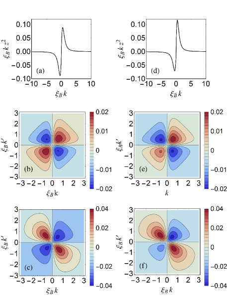
Figure 1: (Color online) The phonon momentum density $kz_{k}^{2}$, the density correlation $\rho_{k,k^{\prime}}$, and the pair correlation $\kappa_{k,k^{\prime}}$ characterizing a many-phonon system. The first column is for the polaron ground state ($p=0$) and the second column is for a polaron state at finite momentum $p\xi_{B}=1.5$. Both columns have $m_{B}/m_{I}=1$ and $\alpha^{(1)}=2$.

displays an example with $p=0$, $m_{B}/m_{I}=1$, and $\alpha^{(1)}=2$. Interesting details emerge from the 2D contour plots of $\rho_{kk^{\prime}}$ and $\kappa_{kk^{\prime}}$ in Figs. 1(b) and 1(c). First, the vertical and horizontal lines at $k=0$ and $k^{\prime}=0$ are the zero contour lines along which the correlation functions vanish or are “transparent.” This “transparency” occurs because the effective phonon interaction in momentum space is given by $kk^{\prime}/m_{I}$ [Eq. (7)] and thus vanishes when $k=0$ or $k^{\prime}=0$. Second, the $k=0$ and $k^{\prime}=0$ lines divide each contour plot into two regions, one with $kk^{\prime}>0$ (the first and third quadrants) and the other with $kk^{\prime}<0$ (the second and fourth quadrants). Each correlation is seen to have opposite signs in these two regions. Third, correlations develop peaks near but not at the origin, along the positive diagonal ($k=k^{\prime}$) and negative diagonal ($k=-k^{\prime}$), but decrease rapidly towards zero as momentum increases. This can be explained as follows. As $k$ and $k^{\prime}$ increase, phonons interact more strongly, but are tuned farther away from resonance, owing to an increase in the effective single-phonon energy, $\mathcal{C}_{i}$ [Eq. (20)] in the diagonal elements of matrix $A$ in Eq. (34). In the limit of large $k$ and $k^{\prime}$, being tuned away from resonance dominates and $\rho_{kk^{\prime}}$ and $\kappa_{kk^{\prime}}$ become diminishingly small. The peaks at intermediate momenta are the outcome of the competition between these two opposing factors.

The second column in Fig. 1 is the same as the first column except $p=1.5\xi_{B}^{-1}$, e.g. a polaronic system prepared adiabatically from one in which the impurity has a momentum $p=1.5\xi_{B}^{-1}$. In contrast to the $p=0$ case, where $p_{ph}=0$ and all diagrams [Figs. 1(a), 1(b), and 1(c)] are symmetric, nonzero $p$ leads to nonzero $p_{ph}$ and an asymmetry develops: the $k>0$ peak has a larger magnitude than the $k<0$ peak for $kz_{k}^{2}$ in Fig. 1(d), with similar scenarios for the peaks along the diagonal elements of the correlation functions, $\rho_{kk}$ and $\kappa_{kk}$ in Figs. 1(e) and 1(f). This is consistent with the expectation that for nonzero $p$, a moving impurity drags a phonon cloud with it, leading to nonzero phonon momentum $p_{ph}$. However, nonzero $p$ does not affect the symmetry of correlations between opposite momenta, $\rho_{k,-k}$ and $\kappa_{k,-k}$, as can be seen in Figs. 1(e) and 1(f). The reason is that $\rho$ and $\kappa$ are symmetric matrices and therefore $\rho_{k,-k}$ and $\kappa_{k,-k}$ must be even functions of $k$, independent of $p$.

In order to better understand the phonon cloud, such as the statistical character of the quantum fluctuations, we follow shchadilova14arXiv:1410.5691 and examine

$$g_{kk^{\prime}}^{\left(2\right)}=\frac{\left\langle\hat{b}_{k}^{{\dagger}}\hat{b}_{k^{\prime}}^{{\dagger}}\hat{b}_{k^{\prime}}\hat{b}_{k}\right\rangle}{\left\langle\hat{b}_{k}^{{\dagger}}\hat{b}_{k}\right\rangle\left\langle\hat{b}_{k^{\prime}}^{{\dagger}}\hat{b}_{k^{\prime}}\right\rangle},$$ (41)

which is the multi-mode generalization of the single-mode second-order correlation, $g_{kk}^{(2)}$, popular in the study of quantum optics Walls and Milburn (2008), where $\langle\hat{b}_{k}^{{\dagger}}\hat{b}_{k^{\prime}}\rangle=z_{k}z_{k^{\prime}}+\rho_{kk^{\prime}}$ and $\langle\hat{b}_{k}^{{\dagger}}\hat{b}_{k^{\prime}}^{{\dagger}}\hat{b}_{k^{\prime}}\hat{b}_{k}\rangle=(z_{k}z_{k^{\prime}}+\kappa_{kk^{\prime}})^{2}+z_{k}^{2}\rho_{k^{\prime}k^{\prime}}+z_{k^{\prime}}^{2}\rho_{kk}+2z_{k}z_{k^{\prime}}\rho_{kk^{\prime}}+\rho_{kk^{\prime}}^{2}+\rho_{kk}\rho_{k^{\prime}k^{\prime}}$, which are valid when quantities are real. In Fig. 2,

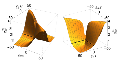
Figure 2: (Color online) Two perspectives for the second order correlation function $g_{k,k^{\prime}}^{(2)}$ as a function of $k$ and $k^{\prime}$ for the example in the first column of Fig. 1.

the thick black lines passing through the origin indicate the $g_{kk^{\prime}}^{(2)}=1$ plane (not shown), which is the value of $g_{kk^{\prime}}^{(2)}$ if phonons are prepared in a MF coherent state. The region $kk^{\prime}<0$ exhibits phonon bunching, $g_{kk^{\prime}}^{(2)}>1$, while the region $kk^{\prime}>0$ exhibits phonon anti-bunching, $g_{kk^{\prime}}^{(2)}<1$. In particular, $g_{k,-k}^{(2)}$ decreases from 1 and saturates at a value less than 1 while $g_{k,k}^{(2)}$ increases from 1 and saturates at a value larger than $1$, a phenomenon first observed in an analogous 3D model shchadilova14arXiv:1410.5691 and is believed to be accessible by noise correlation analysis in time-of-flight experiments Altman et al. (2004); Folling et al. (2005); Rom et al. (2006). A qualitative explanation may be that in the region $kk^{\prime}<0$, the phonon interaction is attractive and thus tends to cause phonons to cluster, leading to phonon bunching, while in the region $kk^{\prime}>0$, the phonon interaction is repulsive and thus tends to cause phonons to spread, leading to phonon anti-bunching.

III.2 Polaron Energy

Having discussed the variables parameterizing the polaron, we now investigate the polaron energy for a system with total momentum $p$. The polaron energy was given in Eq. (15), which may be simplified, with the help of Eqs. (21) and (18), to

$$E_{p} =\frac{p^{2}}{2m_{I}}+\frac{1}{\sqrt{\mathcal{V}}}\sum_{i}g_{{}_{i}}z_{i}-\frac{p_{ph}^{2}}{2m_{I}}$$

$$\qquad+\sum_{i}\mathcal{C}_{i}\rho_{ii}+\frac{1}{2m_{I}}\sum_{i,j}\left(k_{i}k_{j}\right)\left(\kappa_{ij}^{2}+\rho_{ij}^{2}\right),$$ (42)

which is valid in equilibrium where all variables are real.

As in the previous subsection, we begin with the MF limit where the trial state is chosen as a product of coherent states parameterized by only $z_{k}$. In this limit, the polaron energy (42) may be evaluated analytically and gives (where $\bar{E}_{p}\equiv E_{p}/[\hbar^{2}/(m_{B}\xi_{B}^{2})]$)

$$\bar{E}_{p} =\frac{\bar{m}_{B}}{2}\bar{p}^{2}-\frac{\bar{m}_{B}}{2}\bar{p}_{ph}^{2}-\frac{\alpha^{\left(1\right)}}{2}\frac{\bar{m}_{B}^{2}}{\sqrt{\left|\bar{r}\right|}}\left(1+\frac{1}{\bar{m}_{B}}\right)^{2}$$

$$\quad\times\left\{\begin{array}[]{ll}\coth^{-1}\frac{1+\bar{m}_{B}+\bar{b}}{\sqrt{\left|\bar{r}\right|}}+\coth^{-1}\frac{1+\bar{m}_{B}-\bar{b}}{\sqrt{\left|\bar{r}\right|}}&\text{ if }\bar{r}>0\\ \cot^{-1}\frac{1+\bar{m}_{B}+\bar{b}}{\sqrt{\left|\bar{r}\right|}}+\cot^{-1}\frac{1+\bar{m}_{B}-\bar{b}}{\sqrt{\left|\bar{r}\right|}}&\text{ if }\bar{r}<0,\end{array}\right.$$ (45)

which changes smoothly across $\bar{r}=0$ at which $\bar{E}_{p}=\bar{m}_{B}[\bar{p}^{2}-\bar{p}_{ph}^{2}-\alpha^{\left(1\right)}\left(1+\bar{m}_{B}^{-1}\right)^{2}]/2$. The polaron energy $\bar{E}_{p}$ depends on the total momentum $p$. However, it has been long established Spohn (1986) that the ground state, where the polaron energy is lowest, occurs at $p=0$. This is a general statement, and is thus true for both the HFB and MF descriptions. For the MF description, the ground state polaron energy is then obtained from Eq. (45) by setting $p=0$:

$$\bar{E}_{0}=-\alpha^{\left(1\right)}\frac{\left(1+\bar{m}_{B}\right)^{2}}{\sqrt{\left|\bar{m}_{B}^{2}-1\right|}}\left\{\begin{array}[]{ll}\coth^{-1}\frac{1+\bar{m}_{B}}{\sqrt{\left|\bar{m}_{B}^{2}-1\right|}}&\text{ if }\bar{m}_{B}>1\\ \cot^{-1}\frac{1+\bar{m}_{B}}{\sqrt{\left|\bar{m}_{B}^{2}-1\right|}}&\text{ if }\bar{m}_{B}<1,\end{array}\right.$$ (46)

and $\bar{E}_{0}=-2\alpha^{(1)}$ when $\bar{m}_{B}=1$.

We benchmark our HFB model by comparing its prediction for the ground state polaron energy with the predictions from MF theory (46) and Feynman’s path integral formalism, which was regarded as a superior all coupling approximation Tempere et al. (2009). Feynman’s method amounts to applying the Feynman-Jensen inequality on a variational action describing two (classical) particles coupled via a harmonic force, where one is the impurity and the other is a fictitious particle. Steps involved in integrating out the degrees of freedom for the fictitious particle leading to an effective variational action for the impurity are highlighted in Appendix A.

The first column in Fig. 3

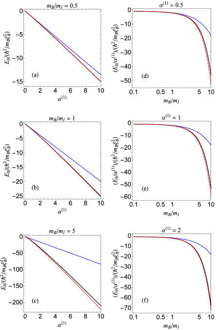
Figure 3: (Color online) The first column displays the ground state polaron energy $E_{0}$ in units of $\hbar^{2}/\left(m_{B}\xi_{B}^{2}\right)$ as a function of the dimensionless polaronic coupling constant $\alpha^{\left(1\right)}$ when (a) $m_{B}/m_{I}=0.5$, (b) $1$, and (c) $5$. The second column shows the polaron energy divided by $\alpha^{\left(1\right)},$ $E_{0}/\alpha^{\left(1\right)}$, in units of $\hbar^{2}/\left(m_{B}\xi_{B}^{2}\right)$ as a function of the boson-impurity mass ratio, $m_{B}/m_{I}$, when (d) $\alpha^{\left(1\right)}=0.5$, (e) $1$, and (f) $5$. In each plot the solid black curve is our HFB result, the dashed blue curve is the MF result, and the dash-dotted red curve is Feynman’s path integral result.

displays the ground state polaron energy, $\bar{E}_{0}$, as a function of the coupling constant $\alpha^{(1)}$ for various boson-impurity mass ratios, $\bar{m}_{B}=m_{B}/m_{I}$. The dashed blue curves are obtained from the MF theory [Eq. (46)], the solid black curves are obtained from our HFB theory, and the dash-dotted red curves from Feynman’s path integral formalism. The MF variational ansatz for finite $\bar{m}_{B}$ is motivated by the observation that the MF theory becomes exact in the limit of heavy impurity $\bar{m}_{B}\rightarrow 0$, where $\hat{H}_{int}$ in Eq. (6) is negligible and the shifting operation (9) with $z_{k}=-(g_{k}/\omega_{k})/\sqrt{\mathcal{V}}$ alone can diagonalize Eq. (6). Indeed, results from all three approaches, although not shown, would be plotted virtually atop one another for roughly $\bar{m}_{B}<0.2$. As the impurity becomes increasingly less massive, i.e. $\bar{m}_{B}$ increases, Figs. 3(a), 3(b), and 3(c) illustrate that the MF results become increasingly larger than Feynman’s, in sharp contrast to the HFB results which match nicely with Feynman’s, demonstrating that correlations, which are excluded from the MF theory, are an important part of the ground polaron state

The second column in Fig. 3 displays $\bar{E}_{0}/\alpha^{(1)}$ as a function of the mass ratio, $\bar{m}_{B}$, for various values of the coupling constant $\alpha^{(1)}$. Equation (46) tells us the MF $\bar{E}_{0}$ is proportional to $\alpha^{(1)}$ and thus $\bar{E}_{0}/\alpha^{(1)}$ is independent of $\alpha^{(1)}$, as illustrated by identical dashed curves in the second column. In the limit of heavy impurity mass, Eq. (46) asymptotes to

$$\bar{E}_{0}/\alpha^{\left(1\right)}\approx-\frac{\pi}{4}+\frac{1}{2}\bar{m}_{B}-\frac{5\pi}{8}\bar{m}_{B}^{2}+\cdots,$$ (47)

where, as explained above, the MF result becomes an exact solution. As can be seen from the second column, the HFB and Feynman results agree very well with the MF results in this limit. In the limit of light impurity, Eq. (46) asymptotes to

$$\frac{\bar{E}_{0}}{\alpha^{\left(1\right)}}\approx-\ln\left(2\bar{m}_{B}\right)\left(\frac{\bar{m}_{B}}{2}+1\right)+\frac{1-6\ln\left(2\bar{m}_{B}\right)}{8\bar{m}_{B}}+\cdots.$$ (48)

In this case we do not expect the MF result to be accurate and we find again that the HFB and Feynman results disagree strongly with the MF results but agree well with each other, indicating as before that neglecting quantum fluctuations in the light impurity limit can lead to significant errors. The HFB and Feynman energies are seen to decrease rapidly with decreasing impurity mass (increasing $\bar{m}_{B}$), while the MF energy changes slowly due to the existence of a logarithmic function in the leading term in Eq. (48).

III.3 Effective Polaron Mass

Finally, we turn our attention to the effective polaron mass $m_{I}^{\ast}$ defined by

$$m_{I}^{\ast}=\left(\left.\frac{\partial^{2}E_{p}}{\partial p^{2}}\right|_{p=0}\right)^{-1},$$ (49)

which follows from expansion of the polaron energy through second order in the total momentum $p$, $E_{p}\approx E_{0}+p^{2}/2m_{I}^{\ast}$, where $E_{0}$ is the ground state polaron energy studied in Fig. 3. $m_{I}^{\ast}$ emerges naturally from Landau’s concept of a mobile polaron, in which an impurity drags with it a cloud of nearby background particles, leading to an effective mass $m_{I}^{\ast}$ heavier than its bare mass $m_{I}$. This picture together with the conservation of momentum means the impurity momentum $p_{I}$ equals the total momentum minus the momentum of the phonon cloud $p_{ph}$: $p_{I}=p-p_{ph}$, leading to the formula Shashi et al. (2014)

$$\frac{1}{m_{I}^{\ast}}=\frac{1}{m_{I}}-\frac{1}{m_{I}}\lim_{p\rightarrow 0}\frac{p_{ph}}{p},\text{ }$$ (50)

which is consistent with Eq. (49).

Figure 4

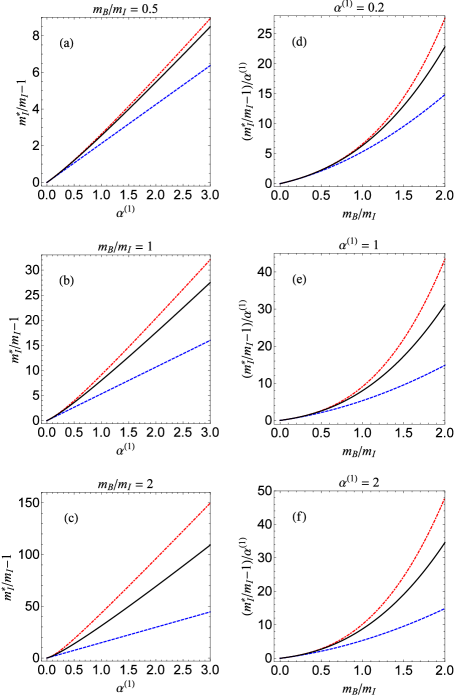
Figure 4: (Color online) A comparison of effective polaron masses according to MF theory (dashed blue curves), our HFB theory (solid black curves), and Feynman’s variational method (dash-dotted red curves). In the first column, $m_{I}^{\ast}/m_{I}-1$ is plotted as a function of $\alpha^{(1)}$ for (a) $m_{B}=0.5$, (b) $1.0$, and (c) $2.0$. In the second column, $(m_{I}^{*}/m_{I}-1)/\alpha^{(1)}$ is plotted as a function of $m_{B}/m_{I}$ for (d) $\alpha^{(1)}=0.5$, (e) $1.0$, and (f) $2.0$.

displays the effective polaron mass $m_{I}^{\ast}$. We show $\bar{m}_{I}^{\ast}$ as a function of $\alpha^{\left(1\right)}$ for various values of $\bar{m}_{B}$ in the first column and as a function of $\bar{m}_{B}$ for various values of $\alpha^{\left(1\right)}$ in the second column. In both columns the solid black curves are from our HFB method, and the dashed blue curves are from the MF theory, which, as in the previous subsection, can be computed analytically:

$$\bar{m}_{I}^{\ast}=1+\frac{2\alpha^{\left(1\right)}\bar{m}_{B}^{2}\left(1+\bar{m}_{B}\right)}{\bar{m}_{B}-1}+\frac{4\alpha^{\left(1\right)}\bar{m}_{B}\left(1+\bar{m}_{B}\right)}{\left(\bar{m}_{B}-1\right)\sqrt{\left|\bar{m}_{B}^{2}-1\right|}}$$

$$\times\left\{\begin{array}[]{ll}\tanh^{-1}\frac{1+\bar{m}_{B}}{\sqrt{\left|\bar{m}_{B}^{2}-1\right|}}-\tanh^{-1}\frac{\bar{m}_{B}}{\sqrt{\left|\bar{m}_{B}^{2}-1\right|}}&\text{ if }\bar{m}_{B}>1,\\ -\tan^{-1}\frac{1+\bar{m}_{B}}{\sqrt{\left|\bar{m}_{B}^{2}-1\right|}}+\tan^{-1}\frac{\bar{m}_{B}}{\sqrt{\left|\bar{m}_{B}^{2}-1\right|}}&\text{ if }\bar{m}_{B}<1,\end{array}\right.$$ (53)

and $\bar{m}_{I}^{\ast}=1+\frac{16}{3}\alpha^{(1)}$ if $\bar{m}_{B}=1$. Figure 4 also includes the effective mass obtained from Feynman’s approach using Eq. (64) in Appendix A as the dash-dotted red curves. Figure 4 demonstrates that the HFB theory consistently gives a heavier effective mass than the MF theory and that it can be significantly heavier for small $\bar{m}_{B}$ or large $\alpha^{(1)}$. The effective mass using Feynman’s method, while consistently heavier than in both methods, is much closer to our HFB result, once again demonstrating the nonclassical nature of the phonon cloud inside of which phonons are highly correlated. A difference between Feynman’s and our HFB masses is expected since Feynman’s approach cannot compute the polaron energy at finite $p$ and hence defines the effective mass differently from Eq. (49).

We conclude this subsection by noting that in the heavy impurity limit, Eq. (64) is found numerically to agree with the MF result

$$\bar{m}_{I}^{\ast}\approx 1+\alpha^{\left(1\right)}\pi\bar{m}_{B}+\alpha^{\left(1\right)}\left(2\pi-4\right)\bar{m}_{B}^{2}+\cdots,$$ (54)

while the variational mass $M$ is found to depart significantly from the above MF result. Thus, in Feynman’s method, $M$ does not agree with the effective polaron mass formula in Eq. (64) and we must use Eq. (64) to compute the effective polaron mass.

IV Conclusion

We considered the Fröhlich model in a moving frame defined by the LLP transformation, where the original impurity-phonon system is transformed to an interacting many-phonon system free of impurities. This LLP model distinguishes itself with the four-boson interaction term in Eq. (7) where an interaction between two phonons with momentum $\mathbf{k}$ and $\mathbf{k}^{\prime}$ does not involve any momentum exchange and is facilitated by a “potential” that depends on $\mathbf{k}\cdot\mathbf{k}^{\prime}$. In the spirit of generalized HFB theory, we formulated a field theoretical description of the LLP model where phonons are subject to this unique phonon-phonon interaction. As an application, we applied our theory to Bose polarons in quasi-1D cold atom mixtures and investigated polaron properties such as energy and mass by solving the HFB equations self-consistently and the HFB equations in the MF limit analytically.

We found in the regime of relatively light impurity and strong coupling, our HFB results were significantly closer to those from Feynman’s method than predictions from MF theory. The agreement between our HFB approach and Feynman’s method on the polaron energy was particularly impressive. We found in the strongly interacting region that the polaron ground state contains highly correlated phonon pairs. In any many-body system at (or close to) zero temperature, the exact nature of the ground state depends crucially on how particles interact with each other. We attributed the existence of both repulsive (in the region $kk^{\prime}>0$) and attractive (in the region $kk^{\prime}<0$) phonon-phonon interactions to the rich structure exhibited in various correlation functions, and to bunching and anti-bunching statistics exhibited in the second-order correlation function.

We expect the 3D polaron to behave differently than our 1D polaron since their densities of states differ. Nevertheless, it is worth pointing out that for the 3D polaron, as the polaron coupling constant increases the ground state energy first rises above the impurity-condensate interaction energy and then decreases below it, while in our 1D case the ground state energy is always below it and decreases monotonically with increasing $\alpha^{\left(1\right)}$. This difference may be traced to the fact that the 3D case suffers from an ultraviolet divergence, a complication that does not occur in our 1D model. As a result, the 1D system has allowed us to focus our attention on our main purpose: gaining clean insight into the role the effective phonon-phonon interaction and quantum fluctuations play in polaronic states.

Finally, we comment that the recent upsurge of interest in Bose polarons has been largely spurred by the prospect that the rich toolbox and the flexibility of cold atom systems may allow polaron theories to be tested, to great precision, in cold atom experiments. However, many observables, which occur as correlation functions involving various field operators, are inaccessible to Feynman’s method. Our HFB theory, however, can cast these observables into forms which are, at least in principle, amenable to numerical analysis. As a concrete example, in Appendix B we express, in terms of the variational parameters of polarons, a time-dependent overlap function that lies at the heart of radio-frequency (rf) spectroscopy, which has emerged as a powerful tool in the study of cold atom physics in general and polaron physics in particular.

Appendix A Feynman’s Variational Approach

In this appendix, we outline Feynman’s variational approach to the polaron Feynman (1955), beginning with the partition function, $Z=$Tr$(e^{-\beta\hat{H}^{\prime}})$, where $\hat{H}^{\prime}$ is given by Eq. (1) and $k_{B}\beta$ equals the inverse temperature. Tracing out the bosonic degrees of freedom gives rise to an effective action for the impurity

$$S =\int_{0}^{\beta}d\tau\frac{1}{2}m_{I}\mathbf{\dot{r}}^{2}\left(\tau\right)-\frac{1}{2\mathcal{V}}\sum_{\mathbf{k}}g_{\mathbf{k}}^{2}$$

$$\quad\times\int_{0}^{\beta}\int_{0}^{\beta}d\tau d\sigma\mathcal{G}\left(\omega_{\mathbf{k}},\left|\tau-\sigma\right|\right)e^{i\mathbf{k}\cdot\left[\mathbf{r}\left(\tau\right)-\mathbf{r}\left(\sigma\right)\right]},$$ (55)

where

$$\mathcal{G}\left(x,u\right)=\cosh\left[x\left(u-\beta/2\right)\right]/\sinh\left(\beta x/2\right),$$ (56)

with $\omega_{\mathbf{k}}$ and $g_{\mathbf{k}}$ given in Eqs. (2) and (3), respectively.

To compute the ground state free energy, $F$, of the Fröhlich Hamiltonian $\hat{H}^{\prime}$ in Eq. (1) [hence the action in Eq. (55)], Feynman introduces a novel variational approach based on the Feynman-Jensen inequality,

$$F\leq F_{var}-\left\langle S-S_{var}\right\rangle_{S_{var}},$$ (57)

where $F_{var}$ is the free energy of a variational system and the average in $\langle S-S_{var}\rangle_{S_{var}}$ is performed with respect to the variational system’s ground state. Minimizing the right-hand side of Eq. (57) gives the strongest bound on $F$, which we take to be our estimate of $F$. As a variational system, Feynman uses the impurity interacting with a fictitious particle via a harmonic potential. Integrating out the fictitious particle yields the variational action for the impurity:

$$S_{var} =\int_{0}^{\beta}d\tau\frac{1}{2}m_{I}\mathbf{\dot{r}}^{2}\left(\tau\right)+\frac{MW^{3}}{8}$$

$$\times\int_{0}^{\beta}\int_{0}^{\beta}d\tau d\sigma\mathcal{G}\left(W,\left|\tau-\sigma\right|\right)\left[\mathbf{r}\left(\tau\right)-\mathbf{r}\left(\sigma\right)\right]^{2},$$ (58)

where $M$, the mass of the fictitious particle, and $W$, the frequency of the harmonic potential, are the variational parameters. A straightforward but lengthy calculation gives for the inequality (57) Tempere et al. (2009); Casteels et al. (2012)

$$F \leq\frac{d}{\beta}\left[\ln\sinh\left(\frac{\beta\Omega}{2}\right)-\ln\sinh\left(\frac{\beta\Omega}{2\sqrt{1+M/m_{I}}}\right)\right]$$

$$-\frac{d}{2\beta}\ln\frac{m_{I}+M}{m_{I}}-\frac{d}{2\beta}\frac{M}{m_{I}+M}\left[\frac{\beta\Omega}{2}\coth\frac{\beta\Omega}{2}-1\right]$$

$$-\sum_{\mathbf{k}}g_{\mathbf{k}}^{2}\int_{0}^{\beta/2}du\,\mathcal{G}\left(\omega_{\mathbf{k}},u\right)\mathcal{M}_{M,\Omega}\left(\mathbf{k},u\right),$$ (59)

where $d$ is the dimension, $W$ is replaced in favor of the more convenient $\Omega=W\sqrt{1+(M/m_{I})}$, and

$$\mathcal{M}_{M,\Omega}\left(\mathbf{k},u\right)$$

$$=\exp\left\{-\frac{k^{2}}{2\left(m_{I}+M\right)}\left[u-\frac{u^{2}}{\beta}+\frac{M}{m_{I}\Omega}\left(\cdots\right)\right]\right\},$$ (60)

with $\left(\cdots\right)$ being defined as

$$\left(\cdots\right)=\frac{\cosh\left(\beta\Omega/2\right)-\cosh\left[\Omega\left(\beta/2-u\right)\right]}{\sinh\left(\beta\Omega/2\right)}.$$ (61)

As discussed in the main body of the paper, our interest lies in the zero temperature limit, which simplifies Eq. (59) to

$$E_{0} \leq\frac{\Omega d}{2}-\frac{\Omega d}{2\sqrt{1+M/m_{I}}}-\frac{M\Omega d}{4\left(m_{I}+M\right)}$$

$$-\frac{1}{\mathcal{V}}\sum_{\mathbf{k}}g_{\mathbf{k}}^{2}\int_{0}^{\infty}due^{-u\omega_{\mathbf{k}}}\lim_{\beta\rightarrow\infty}\mathcal{M}_{M,\Omega}\left(\mathbf{k},u\right),$$ (62)

where we have changed the free energy $F$ to the polaron ground state energy $E_{0}$ and

$$\lim_{\beta\rightarrow\infty}\mathcal{M}_{M,\Omega}\left(\mathbf{k},u\right)$$

$$=\exp\left\{-\frac{k^{2}}{2\left(m_{I}+M\right)}\left[u+\frac{M\left(1-e^{-u\Omega}\right)}{m_{I}\Omega}\right]\right\}.$$ (63)

At zero temperature, Feynman Feynman (1955) derived from the asymptotic form of the partition function a formula for the effective polaron mass,

$$m_{I}^{\ast} =m_{I}+\frac{1}{d\mathcal{V}}\sum_{\mathbf{k}}k^{2}g_{\mathbf{k}}^{2}$$

$$\qquad\times\int_{0}^{\infty}due^{-u\omega_{\mathbf{k}}}u^{2}\lim_{\beta\rightarrow\infty}\mathcal{M}_{M,\Omega}\left(\mathbf{k},u\right).$$ (64)

The positive $M$ and $\Omega$ that minimize the right hand side of Eq. (62) for $d=1$ are fed back into the left hand side of Eq. (62) to give the polaron energy $E_{0}$ which we display in Fig. 3. These same values of $M$ and $\Omega$ are then used in Eq. (64) for $d=1$ to compute the effective mass which we display in Fig. 4.

Appendix B RF Spectrum

In this appendix, we establish a framework for calculating the impurity rf spectra Chin et al. (2004); Schirotzek et al. (2009); Feld et al. (2011) in our HFB model. In rf spectroscopy, an rf field of amplitude $F_{L}$ and frequency $\omega_{L}$ is applied to promote the impurity from an initial state $|g\rangle$ to a final state $|e\rangle$, which are internal states, e.g. hyperfine states. The two states differ by energy $\omega_{eg}$ and the process is described by the Hamiltonian $\tilde{H}_{rf}=(F_{L}e^{-i\omega_{L}t}|e\rangle\langle g|+\text{h.c.})/2$. The total Hamiltonian $\tilde{H}$ for this two-state impurity-BEC system is

$$\tilde{H}=\omega_{eg}\left|e\right\rangle\left\langle e\right|+\hat{H}_{gg}\left|g\right\rangle\left\langle g\right|+\hat{H}_{ee}\left|e\right\rangle\left\langle e\right|+\tilde{H}_{rf},$$ (65)

where $\hat{H}_{gg}$ and $\hat{H}_{ee}$ describe impurity-phonon subsystems containing $|g\rangle$-type and $|e\rangle$-type impurities, respectively. The polarization of such a system is expected to oscillate periodically at rf frequency $\omega_{L}$, and the rf (or probe absorption) spectrum is then expected to be proportional to the following expectation value:

$$\operatorname{Re}\left[i\left\langle\left|g\right\rangle\left\langle e\right|\right\rangle e^{i\omega_{L}t}/F_{L}\right].$$ (66)

Let $|i_{g}\rangle$ be the ground state of $\hat{H}_{gg}$ with energy $E_{ig}$ and $|f_{e}\rangle$ be any eigenstate of $\hat{H}_{ee}$ with energy $E_{fe}$. Let $|i_{g},g\rangle$ and $|f_{e},e\rangle$ be the initial and final (impurity-phonon) states of the total system described by $\tilde{H}$ in Eq. (65). Evaluating Eq. (66), within the framework of linear response theory, yields, straightforwardly, the rf spectrum (Fermi’s golden rule),

$$I_{p}\left(\omega\right)=\sum_{f_{e}}\left|\left\langle f_{e},e\right|e\rangle\langle g\left|i_{g},g\right\rangle\right|^{2}\delta\left[\omega-\left(E_{fe}-E_{ig}\right)\right],$$ (67)

where the subscript $p$ on the left-hand side (which we suppress on the right-hand side to reduce clutter) represents the total momentum [first introduced in Eq. (6)] and the frequency $\omega\equiv\omega_{L}-\omega_{eg}$ is measured relative to the $|e\rangle\longleftrightarrow|g\rangle$ atomic transition. A standard manipulation transforms Eq. (67) into an integral Knap et al. (2012)

$$I_{p}\left(\omega\right)=\operatorname{Re}\frac{1}{\pi}\int_{0}^{\infty}dte^{i\omega t}\mathcal{A}_{p}\left(t\right),$$ (68)

involving an overlap function in the time domain defined as

$$\mathcal{A}_{p}\left(t\right)=e^{iE_{ig}t}\left\langle i_{g}\right|e^{-i\hat{H}_{ee}t}\left|i_{g}\right\rangle.$$ (69)

In the (direct) rf measurement, the rf field excites impurities in state $|g\rangle$, which interact with the BEC via $s$-wave scattering, to state $|e\rangle$, where they do not interact with the BEC. In this case, $\hat{H}_{gg}$ is the interacting phonon Hamiltonian in Eq. (6), $\hat{H}_{ee}$ is the free phonon Hamiltonian $\hat{H}_{ee}=\sum_{\mathbf{k}}\omega_{\mathbf{k}}\hat{b}_{\mathbf{k}}^{{\dagger}}\hat{b}_{\mathbf{k}}$ Shashi et al. (2014), $E_{ig}$ is the polaron energy $E_{p}$ in Eq. (15), and $|i_{g}\rangle$ is the polaron state $|\phi\rangle$ introduced in Sec. II.

To facilitate the evaluation of Eq. (69), we express the polaron state $|\phi\rangle$ in terms of the phonon vacuum $|0\rangle$ Blaizot and Ripka (1986)

$$\left|\phi\right\rangle=\frac{\exp\frac{1}{2}\sum_{\mathbf{kk}^{\prime}}\hat{c}_{\mathbf{k}}^{{\dagger}}\left(G_{\mathbf{kk}^{\prime}}^{\ast}\equiv\left(U^{\ast-1}V^{\ast}\right)_{\mathbf{kk}^{\prime}}\right)\hat{c}_{\mathbf{k}^{\prime}}^{{\dagger}}}{\left[\det\left(U^{{\dagger}}U\right)\right]^{1/4}}\left|0\right\rangle,$$ (70)

and at the same time organize $\exp(-i\hat{H}_{ee}t)$ into an antinormal ordered form Louisell (1990)

$$\exp\left(-i\hat{H}_{ee}t\right)={\displaystyle\prod_{\mathbf{k}}}\sum_{m=0}^{\infty}\frac{\left(1-\exp\left(i\omega_{\mathbf{k}}t\right)\right)^{m}}{m!}$$

$$\qquad\times\exp\left(i\omega_{\mathbf{k}}t\right)\left(z_{\mathbf{k}}+\hat{c}_{\mathbf{k}}\right)^{m}\left(z_{\mathbf{k}}^{\ast}+\hat{c}_{\mathbf{k}}^{{\dagger}}\right)^{m}.$$ (71)

Let $|c_{\mathbf{k}}\rangle$ be the coherent state of $\hat{c}_{\mathbf{k}}$, i.e. $\hat{c}_{\mathbf{k}}|c_{\mathbf{k}}\rangle=c_{\mathbf{k}}|c_{\mathbf{k}}\rangle,$ normalized according to $\langle c_{\mathbf{k}}|0\rangle=1$. In the coherent state space defined by the completeness relation

$${\displaystyle\prod_{\mathbf{k}}}\int\frac{dc_{\mathbf{k}}^{\ast}dc_{\mathbf{k}}}{2\pi i}e^{-c_{\mathbf{k}}c_{\mathbf{k}}^{\ast}}\left|c_{\mathbf{k}}\right\rangle\left\langle c_{\mathbf{k}}\right|=I,$$ (72)

we can cast the overlap function, $\mathcal{A}_{p}\left(t\right)=e^{iE_{p}t}\left\langle\phi\right|e^{-i\hat{H}_{ee}t}\left|\phi\right\rangle,$ into a Gaussian integral

$$\mathcal{A}_{p}\left(t\right) =\exp\sum_{\mathbf{k}}\left[i\omega_{\mathbf{k}}t+\left(1-e^{i\omega_{\mathbf{k}}t}\right)\left|z_{\mathbf{k}}\right|^{2}\right]$$

$$\qquad\times\frac{e^{iE_{p}t}}{\sqrt{\det\left(U^{{\dagger}}U\right)}}{\displaystyle\prod_{\mathbf{k}}}\int\frac{dc_{\mathbf{k}}^{\ast}dc_{\mathbf{k}}}{2\pi i}e^{h},$$ (73)

where

$$h=-c^{\ast}Kc+\frac{1}{2}cGc+\frac{1}{2}c^{\ast}G^{\ast}c^{\ast}+xc+y^{\ast}c^{\ast},$$ (74)

or explicitly

$$\mathcal{A}_{p}\left(t\right) =e^{iE_{p}t}\frac{\exp\sum_{\mathbf{k}}\left[i\omega_{\mathbf{k}}t+\left(1-e^{i\omega_{\mathbf{k}}t}\right)\left|z_{\mathbf{k}}\right|^{2}\right]}{\sqrt{\det\left(U^{{\dagger}}U\right)}}$$

$$\times\frac{\exp\left\{\frac{1}{2}\left(x,y^{\ast}\right)\left(\begin{array}[c]{cc}K&G^{\ast}\\ G&K\end{array}\right)^{-1}\left(\begin{array}[c]{c}y^{\ast}\\ x\end{array}\right)\right\}}{\sqrt{\det\left(\begin{array}[c]{cc}K&G^{\ast}\\ G&K\end{array}\right)}},$$ (81)

where $K$ is a diagonal matrix defined as

$$K_{ij}=\exp\left(i\omega_{\mathbf{k}_{i}}t\right)\delta_{i,j},$$ (82)

and $x$ and $y$ are vectors defined as

$$x_{i} =\left(1-\exp\left(i\omega_{\mathbf{k}_{i}}t\right)\right)z_{\mathbf{k}_{i}}^{\ast},$$ (83)

$$y_{i} =\left(1-\exp\left(-i\omega_{\mathbf{k}_{i}}t\right)\right)z_{\mathbf{k}_{i}}^{\ast}.$$ (84)

Equation (81) is the main result of this appendix, which expresses the overlap function (69) and hence the rf spectrum (68) in terms of the variables that parametrize the HFB variational polaron state. This may be extended, using the time-dependent HFB variational principle, to inverse rf spectroscopy Kohstall et al. (2012); Shashi et al. (2014), where the rf field transfers impurities in state $|g\rangle$, which do not interact with the BEC, to state $|e\rangle$, where they do interact with the BEC. We leave this as a possible future research project.

References

- Schirotzek et al. (2009) A. Schirotzek, C.-H. Wu, A. Sommer, and M. W. Zwierlein, Phys. Rev. Lett. 102, 230402 (2009).
- Nascimbène et al. (2009) S. Nascimbène, N. Navon, K. J. Jiang, L. Tarruell, M. Teichmann, J. McKeever, F. Chevy, and C. Salomon, Phys. Rev. Lett. 103, 170402 (2009).
- Prokof’ev and Svistunov (2008) N. Prokof’ev and B. Svistunov, Phys. Rev. B 77, 020408 (2008).
- Mora and Chevy (2009) C. Mora and F. Chevy, Phys. Rev. A 80, 033607 (2009).
- Chevy and Mora (2010) F. Chevy and C. Mora, Rep. Prog. Phys. 73, 112401 (2010).
- (6) P. Massignan, M. Zaccanti, and G. M. Bruum, Rep. Prog. Phys. 77, 034401 (2014).
- Jørgensen et al. (2016) N. B. Jørgensen, L. Wacker, K. T. Skalmstang, M. M. Parish, J. Levinsen, R. S. Christensen, G. M. Bruun, and J. J. Arlt, arXiv:1604.07883 (2016).
- Hu et al. (2016) M.-G. Hu, M. J. V. de Graaff, D. Kedar, J. P. Corson, E. A. Cornell, and D. S. Jin, arXiv:1605.00729 (2016).
- Huang and Wan (2009) B.-B. Huang and S.-L. Wan, Chinese Physics Letters 26, 080302 (2009).
- Shashi et al. (2014) A. Shashi, F. Grusdt, D. A. Abanin, and E. Demler, Phys. Rev. A 89, 053617 (2014).
- Kain and Ling (2014) B. Kain and H. Y. Ling, Phys. Rev. A 89, 023612 (2014).
- Cucchietti and Timmermans (2006) F. M. Cucchietti and E. Timmermans, Phys. Rev. Lett. 96, 210401 (2006).
- Sacha and Timmermans (2006) K. Sacha and E. Timmermans, Phys. Rev. A 73, 063604 (2006).
- Casteels et al. (2011a) W. Casteels, T. Cauteren, J. Tempere, and J. T. Devreese, Laser Physics 21, 1480 (2011a), ISSN 1555-6611.
- Laudan and Pekar (1946) L. D. Laudan and S. I. Pekar, Zh. Eksp. Teor. Fiz 16, 341 (1946).
- Laudan and Pekar (1948) L. D. Laudan and S. I. Pekar, Zh. Eksp. Teor. Fiz 18, 419 (1948).
- Tempere et al. (2009) J. Tempere, W. Casteels, M. K. Oberthaler, S. Knoop, E. Timmermans, and J. T. Devreese, Phys. Rev. B 80, 184504 (2009).
- Feynman (1955) R. P. Feynman, Phys. Rev. 97, 660 (1955).
- Li and Das Sarma (2014) W. Li and S. Das Sarma, Phys. Rev. A 90, 013618 (2014).
- Levinsen et al. (2015) J. Levinsen, M. M. Parish, and G. M. Bruun, Phys. Rev. Lett. 115, 125302 (2015).
- Chevy (2006) F. Chevy, Phys. Rev. A 74, 063628 (2006).
- Vlietinck et al. (2015) J. Vlietinck, W. Casteels, K. V. Houcke, J. Tempere, J. Ryckebusch, and J. T. Devreese, New Journal of Physics 17, 033023 (2015).
- Prokof’ev and Svistunov (1998) N. V. Prokof’ev and B. V. Svistunov, Phys. Rev. Lett. 81, 2514 (1998).
- Mishchenko et al. (2000) A. S. Mishchenko, N. V. Prokof’ev, A. Sakamoto, and B. V. Svistunov, Phys. Rev. B 62, 6317 (2000).
- (25) L. A. Peña Ardila and S. Giorgini, Phs. Rev. A 92, 033612 (2015).
- Rath and Schmidt (2013) S. P. Rath and R. Schmidt, Phys. Rev. A 88, 053632 (2013).
- Christensen et al. (2015) R. S. Christensen, J. Levinsen, and G. M. Bruun, Phys. Rev. Lett. 115, 160401 (2015).
- Fetter (1994) A. L. Fetter, “Quantum Theory of Many-Particle Systems,” McGraw-Hill Book Company, New York (1994).
- Mahan (2000) G. D. Mahan, “Many-Particle Physics,” 3rd ed., Kluwer Academic/Plenum Publishers, New York (2000).
- Fröhlich (1954) H. Fröhlich, Adv. Phys. 3, 325 (1954).
- A. S. Alexandrov (2007) A. S. Alexandrov, ed., “Polarons in Advanced Materials,” Springer (2007).
- Casteels et al. (2011b) W. Casteels, J. Tempere, and J. T. Devreese, Phys. Rev. A 83, 033631 (2011b).
- Bruderer et al. (2007) M. Bruderer, A. Klein, S. R. Clark, and D. Jaksch, Phys. Rev. A 76, 011605 (2007).
- Bruderer et al. (2008) M. Bruderer, A. Klein, S. R. Clark, and D. Jaksch, New Journal of Physics 10, 033015 (2008).
- Privitera and Hofstetter (2010) A. Privitera and W. Hofstetter, Phys. Rev. A 82, 063614 (2010).
- Yin et al. (2015) T. Yin, D. Cocks, and W. Hofstetter, Phys. Rev. A 92, 063635 (2015).
- (37) Y. E. Shchadilova, F. Grusdt, A. N. Rubtsov, and E. Demler, Phys. Rev. A 93, 043606 (2016).
- Grusdt et al. (2015) F. Grusdt, Y. E. Shchadilova, A. N. Rubtsov, and E. Demler, Scientific Reports 5, 12124 (2015).
- Grusdt and Demler (2015) F. Grusdt and E. Demler, arXiv:1510.04934 (2015).
- Lee et al. (1953) T. D. Lee, F. E. Low, and D. Pines, Phys. Rev. 90, 297 (1953).
- Kandemir and Altanhan (1994) B. S. Kandemir and T. Altanhan, J. Phys. Condens. Matter 6, 4505 (1994).
- Altanhan and Kandemir (1993) T. Altanhan and B. S. Kandemir, J. Phys. Condens. Matter 5, 6729 (1993).
- (43) A. C. Hewson, “The Kondo Problem to Heavy Fermions”, Cambridge, UK (1997).
- Bloch et al. (2008) I. Bloch, J. Dalibard, and W. Zwerger, Rev. Mod. Phys. 80, 885 (2008).
- Schreck et al. (2001) F. Schreck, L. Khaykovich, K. L. Corwin, G. Ferrari, T. Bourdel, J. Cubizolles, and C. Salomon, Phys. Rev. Lett. 87, 080403 (2001).
- Truscott et al. (2001) A. G. Truscott, K. E. Strecker, W. I. McAlexander, G. B. Partridge, and R. G. Hulet, Science 291, 2570 (2001).
- Ferrier-Barbut et al. (2014) I. Ferrier-Barbut, M. Delehaye, S. Laurent, A. T. Grier, M. Pierce, B. S. Rem, F. Chevy, and C. Salomon, Science 345, 1035 (2014).
- Hadzibabic et al. (2002) Z. Hadzibabic, C. A. Stan, K. Dieckmann, S. Gupta, M. W. Zwierlein, A. Görlitz, and W. Ketterle, Phys. Rev. Lett. 88, 160401 (2002).
- Stan et al. (2004) C. A. Stan, M. W. Zwierlein, C. H. Schunck, S. M. F. Raupach, and W. Ketterle, Phys. Rev. Lett. 93, 143001 (2004).
- Schuster et al. (2012) T. Schuster, R. Scelle, A. Trautmann, S. Knoop, M. K. Oberthaler, M. M. Haverhals, M. R. Goosen, S. J. J. M. F. Kokkelmans, and E. Tiemann, Phys. Rev. A 85, 042721 (2012).
- Ferrari et al. (2002) G. Ferrari, M. Inguscio, W. Jastrzebski, G. Modugno, G. Roati, and A. Simoni, Phys. Rev. Lett. 89, 053202 (2002).
- Roati et al. (2002) G. Roati, F. Riboli, G. Modugno, and M. Inguscio, Phys. Rev. Lett. 89, 150403 (2002).
- Inouye et al. (2004) S. Inouye, J. Goldwin, M. L. Olsen, C. Ticknor, J. L. Bohn, and D. S. Jin, Phys. Rev. Lett. 93, 183201 (2004).
- Ferlaino et al. (2006) F. Ferlaino, C. D’Errico, G. Roati, M. Zaccanti, M. Inguscio, G. Modugno, and A. Simoni, Phys. Rev. A 73, 040702 (2006).
- Park et al. (2012) J. W. Park, C.-H. Wu, I. Santiago, T. G. Tiecke, S. Will, P. Ahmadi, and M. W. Zwierlein, Phys. Rev. A 85, 051602 (2012).
- Silber et al. (2005) C. Silber, S. Günther, C. Marzok, B. Deh, P. W. Courteille, and C. Zimmermann, Phys. Rev. Lett. 95, 170408 (2005).
- McNamara et al. (2006) J. M. McNamara, T. Jeltes, A. S. Tychkov, W. Hogervorst, and W. Vassen, Phys. Rev. Lett. 97, 080404 (2006).
- Bloch et al. (2001) I. Bloch, M. Greiner, O. Mandel, T. W. Hänsch, and T. Esslinger, Phys. Rev. A 64, 021402 (2001).
- Modugno et al. (2001) G. Modugno, G. Ferrari, G. Roati, R. J. Brecha, A. Simoni, and M. Inguscio, Science 294, 1320 (2001).
- Catani et al. (2008) J. Catani, L. De Sarlo, G. Barontini, F. Minardi, and M. Inguscio, Phys. Rev. A 77, 011603 (2008).
- Catani et al. (2012) J. Catani, G. Lamporesi, D. Naik, M. Gring, M. Inguscio, F. Minardi, A. Kantian, and T. Giamarchi, Phys. Rev. A 85, 023623 (2012).
- McCarron et al. (2011) D. J. McCarron, H. W. Cho, D. L. Jenkin, M. P. Köppinger, and S. L. Cornish, Phys. Rev. A 84, 011603 (2011).
- Spethmann et al. (2012) N. Spethmann, F. Kindermann, S. John, C. Weber, D. Meschede, and A. Widera, Phys. Rev. Lett. 109, 235301 (2012).
- Schmid et al. (2010) S. Schmid, A. Härter, and J. H. Denschlag, Phys. Rev. Lett. 105, 133202 (2010).
- Olshanii (1998) M. Olshanii, Phys. Rev. Lett. 81, 938 (1998).
- Bergeman et al. (2003) T. Bergeman, M. G. Moore, and M. Olshanii, Phys. Rev. Lett. 91, 163201 (2003).
- Chin et al. (2010) C. Chin, R. Grimm, P. Julienne, and E. Tiesinga, Rev. Mod. Phys. 82, 1225 (2010).
- Casteels et al. (2012) W. Casteels, J. Tempere, and J. T. Devreese, Phys. Rev. A 86, 043614 (2012).
- Peeters and Devreese (1985) F. M. Peeters and J. T. Devreese, Phys. Rev. B 32, 3515 (1985).
- Ring and Schuck (2004) P. Ring and P. Schuck, “The Nuclear Many-Body Problem,” Springer-Verlag Berlin Heidelberg (2004).
- Blaizot and Ripka (1986) J.-P. Blaizot and G. Ripka, “Quantum Theory of Finite Systems,” The MIT Press, Cambridge, Massachusetts (1986).
- Walls and Milburn (2008) D. F. Walls and G. J. Milburn, “Quantum Optics,” Springer-Verlag Berlin Heidelberg (2008).
- Altman et al. (2004) E. Altman, E. Demler, and M. D. Lukin, Phys. Rev. A 70, 013603 (2004).
- Folling et al. (2005) S. Folling, F. Gerbier, A. Widera, O. Mandel, T. Gericke, and I. Bloch, Nature 434, 481 (2005).
- Rom et al. (2006) T. Rom, T. Best, D. van Oosten, U. Schneider, S. Folling, B. Paredes, and I. Bloch, Nature 444, 733 (2006).
- Spohn (1986) H. Spohn, J. Phys. A 19, 533 (1986).
- Chin et al. (2004) C. Chin, M. Bartenstein, A. Altmeyer, S. Riedl, S. Jochim, J. H. Denschlag, and R. Grimm, Science 305, 1128 (2004).
- Feld et al. (2011) M. Feld, B. Froöhlich, E. Vogt, M. Koschorreck, and M. Köhl, Nature 480, 75 (2011).
- Knap et al. (2012) M. Knap, A. Shashi, Y. Nishida, A. Imambekov, D. A. Abanin, and E. Demler, Phys. Rev. X 2, 041020 (2012).
- Louisell (1990) W. H. Louisell, “Quantum Statistical Properties of Radiation,” John Wiley and Sons, New York (1990).
- Kohstall et al. (2012) C. Kohstall, M. Zaccanti, M. Jag, A. Trenkwalder, P. Massignan, G. M. Bruun, F. Schreck, and R. Grimm, Nature 485, 615 (2012).