Network inference in the non-equilibrium steady state

Abstract

Non-equilibrium systems lack an explicit characterisation of their steady state like the Boltzmann distribution for equilibrium systems. This has drastic consequences for the inference of parameters of a model when its dynamics lacks detailed balance. Such non-equilibrium systems occur naturally in applications like neural networks or gene regulatory networks. Here, we focus on the paradigmatic asymmetric Ising model and show that we can learn its parameters from independent samples of the non-equilibrium steady state. We present both an exact inference algorithm and a computationally more efficient, approximate algorithm for weak interactions based on a systematic expansion around mean-field theory. Obtaining expressions for magnetisations, two- and three-point spin correlations, we establish that these observables are sufficient to infer the model parameters. Further, we discuss the symmetries characterising the different orders of the expansion around the mean field and show how different types of dynamics can be distinguished on the basis of samples from the non-equilibrium steady state.

Inverse problems in statistical physics are motivated by the challenges of big data in different fields, especially high-throughput experiments in biology: Can one learn, for instance, the synaptic connections between neurons from observations of neural activity Cocco et al. (2009), or the regulatory interactions between genes from gene expression levels D’haeseleer et al. (2000)? Inverse statistical problems such as these also include the determination of three-dimensional protein structures Weigt et al. (2009), the inference of fitness landscapes diverseFitness , and flocking dynamics Bialek et al. (2012). The paradigmatic inverse statistical problem is the inverse Ising problem, which seeks to infer the parameters of a spin model – external fields and interactions between spins – from observables like magnetisations and spin correlations. For the equilibrium case, which is characterised by symmetric interactions between pairs of spins and detailed balance, a wide range of approaches have been developed on the basis of the Boltzmann distribution diverseInvIsing . Yet in many applications, like neural networks or gene regulatory networks, interactions are generally asymmetric. For instance, a synaptic connection from neuron $A$ to neuron $B$ does not imply a reverse connection back from $B$ to $A$. The resulting non-equilibrium steady state (NESS) lacks detailed balance and is not described by a Boltzmann distribution. We ask if it is possible to learn the parameters of a non-equilibrium model from independent samples of the NESS, even though the probability with which each state of the system occurs in the long-time limit is unknown. Key result of this paper is the identification of observables from which the parameters of a non-equilibrium model can be reconstructed, and a systematic procedure to infer the model parameters based on these observables.

For concreteness, we start with the asymmetric Ising model in discrete time under so-called Glauber dynamics Glauber (1963): At a given time $t$, the state of a system of $N$ binary spins is characterised by variables $s_{i}(t)$ with $i=1,\ldots,N$. The dynamics of spins is defined by randomly picking a spin variable, say $i$, at each time step. The value of that spin variable is then updated, with $s_{i}(t+1)=\pm 1$ sampled from the probability distribution

$$w(s_{i}(t+1)|\boldsymbol{s}(t))=\frac{\exp\{s_{i}(t+1)\theta_{i}(t)\}}{2\cosh(\theta_{i}(t))}\ ,$$ (1)

where the effective local field is

$$\theta_{i}(t)=h_{i}+\sum_{j=1}^{N}J_{ij}s_{j}(t)\ ,$$ (2)

with external fields $h_{i}$ and couplings between spins $J_{ij}$. This dynamics has been used as a model of neural dynamics Derrida et al. (1987) and as a model of gene expression dynamics Bailly-Bechet et al. (2010). Similar to this sequential dynamics that updates one spin after the other, one can define a dynamics with parallel updates, where the updates (1) are carried out simultaneously for all spins.

For a symmetric coupling matrix without self-couplings, the Glauber dynamics (1) converges to the equilibrium state characterised by the Boltzmann distribution ${p_{B}(\mathbf{s})=e^{-\mathcal{H}(\mathbf{s})}/Z}$ with the well-known Ising Hamiltonian ${\mathcal{H}(\mathbf{s})=-\sum_{i}s_{i}(h_{i}+\sum_{j>i}J_{ij}s_{j})}$. (For convenience we have subsumed the inverse temperature into the couplings and fields.) For asymmetric couplings, however, Glauber dynamics (1) converges to a non-equilibrium steady state, which lacks detailed balance and is hard to characterise.

In the inverse problem, the task is to infer the parameters of the asymmetric Ising model, namely the couplings $J_{ij}$ and external fields $h_{i}$ of (2). This is a comparatively easy task when we can observe time series of consecutive states of the system $\boldsymbol{s}(t),\boldsymbol{s}(t+1),\boldsymbol{s}(t+2),\ldots$. Using the dynamical rule (1), the probability of a particular trajectory $\prod_{t}w(\boldsymbol{s}(t+1)|\boldsymbol{s}(t))$ can be written down explicitly and be maximised with respect to the couplings and fields Roudi and Hertz (2011); Zeng et al. (2013) in polynomial time in $N$ and the length of the trajectory. This yields the maximum likelihood estimate of the model parameters. An estimate of the couplings and fields that can be computed even faster has been derived using mean-field theory Roudi and Hertz (2011); Mézard and Sakellariou (2011).

However, there are situations where a time series of the system’s dynamics is not available. An example is genome-wide gene expression levels measured in single cells, a process which involves the physical destruction of cells. In such cases, only independent samples from the non-equilibrium steady state are available. Beyond the practical relevance, it is also a fundamental question whether we can characterise the NESS sufficiently well to solve the inverse problem.

Already elementary arguments show that, unlike in the equilibrium case Ackley et al. (1985); diverseInvIsing , pairwise spin-correlations are insufficient to infer the model parameters: the matrix of pairwise correlations $\langle s_{i}s_{j}\rangle$ is symmetric and has only $N(N-1)/2$ independent entries, whereas there are $N(N-1)$ entries of the asymmetric coupling matrix $J_{ij}$ to be determined (self-interactions $J_{ii}\neq 0$ are excluded). Thus we expect that at least three-point correlations $\langle s_{i}s_{j}s_{k}\rangle$ are required. On the other hand, the information one can extract from single-time measurements in the NESS is limited to the frequencies of the $2^{N}$ different spin configurations. Taking into account the normalisation constraint, there are thus at most $2^{N}-1$ independent observables available to determine the $N(N-1)+N$ parameters of couplings and external fields. This implies that the parameters can only be inferred for $N\geq 5$.

Self-consistent magnetisations and spin-correlations.

In the following, we write the magnetisations and $n$-point spin-correlations self-consistently as single-time expectations in the steady state involving the effective local fields (2). Further, we employ an expansion around a probability distribution factorising in the spins (mean-field theory) to derive magnetisations, two-, and three-point correlations as an explicit function of the couplings and external fields. By inverting either of these relationships we can solve the inverse problem.

We consider the magnetisations $m_{i}\equiv\langle s_{i}\rangle$ in the steady state, and the fluctuations $\delta s_{i}\equiv(s_{i}-m_{i})$ of spins around this mean. By averaging over the statistics (1), we obtain for the magnetisations and the $n$-point connected correlations $C_{i_{1},i_{2},\ldots,i_{n}}\equiv\langle\delta s_{i_{1}}\delta s_{i_{2}}\cdots\delta s_{i_{n}}\rangle$

$$m_{i}=\langle\tanh(\theta_{i})\rangle\equiv\sum_{\boldsymbol{s}}p(\boldsymbol{s}|\mathbf{h},\boldsymbol{J})\tanh(\theta_{i}(\boldsymbol{s},\mathbf{h},\boldsymbol{J}))$$ (3)

$$C_{i_{1},\ldots,i_{n}}=\frac{1}{n}\sum_{k=1}^{n}\left\langle\left(\prod_{\begin{subarray}{c}j=1\\ j\neq k\end{subarray}}^{n}\delta s_{i_{j}}\right)[\tanh(\theta_{i_{k}})-m_{i_{k}}]\right\rangle,$$ (4)

where $\{i_{1},\ldots,i_{n}\}\subset\{1,\ldots N\}$ is a subset of $n$ spins and $p(\boldsymbol{s}|\mathbf{h},\boldsymbol{J})$ denotes the steady-state probability over spin configurations $\boldsymbol{s}$. These equations are a set of self-consistent equations whose left-hand side gives magnetisations and correlations, which together specify the probability distribution $p(\boldsymbol{s}|\mathbf{h},\boldsymbol{J})$ in the the NESS. The right hand sides depend on this distribution via averages over functions of $\theta_{i}=h_{i}+\sum_{j=1}^{N}J_{ij}s_{j}$. A similar result holds for a dynamics with parallel updates ${C_{i_{1},\ldots,i_{n}}^{\text{par}}=\left\langle\prod_{k=1}^{n}[\tanh(\theta_{i_{k}})-m_{i_{k}}]\right\rangle}$. Given independent samples from the steady state, the expectations in (3) and (4) can be evaluated numerically by averaging over the sampled configurations.

An expansion around mean-field theory.

Although the steady-state probability distribution $p(\boldsymbol{s}|\mathbf{h},\boldsymbol{J})$ underlying the expectations is not known, it turns out that its moments can be calculated in a systematic expansion around a distribution factorising in the spins, ${q(\boldsymbol{s}|\mathbf{h}_{q})\equiv p(\boldsymbol{s}|\mathbf{h}_{q},\boldsymbol{J}_{q}=0)}$. In equilibrium statistical physics, this distribution is the well-known mean-field ansatz. Its application to the non-equilibrium setting has been pioneered by Kappen and Spanjers Kappen and Spanjers (2000). As usual in mean-field theory, the external fields ${\mathbf{h}_{q}=\mathbf{h}_{q}(\mathbf{h},\boldsymbol{J}):=\mathbf{h}-\delta\mathbf{h}}$ characterising the mean-field distribution $q(\boldsymbol{s}|\mathbf{h}_{q})$ are fixed by a self-consistent equation for the magnetisations ${\mathbf{m}(\mathbf{h}_{q},\boldsymbol{J}_{q}=0)=\mathbf{m}(\mathbf{h},\boldsymbol{J})}$, so the mean-field distribution yields the same magnetisations as the original model with couplings $\boldsymbol{J}$ and fields $\mathbf{h}$. Considering external fields $\mathbf{h}_{q}+\lambda\delta\mathbf{h}$ and couplings $\lambda\boldsymbol{J}$, one can smoothly interpolate between $\lambda=0$, describing the factorising distribution $q$, to the NESS described by $\lambda=1$. Expanding the moments of this distribution in a Taylor-series around the mean-field distribution $\lambda=0$ gives

$$\mathbf{m}(\mathbf{h},\boldsymbol{J}) = \sum_{k=0}^{\infty}\frac{1}{k!}\frac{\text{d}^{k}\mathbf{m}(\mathbf{h}_{q}+\lambda\delta\mathbf{h},\lambda\boldsymbol{J})}{\text{d}\lambda^{k}}\Big{|}_{\lambda=0}$$ (5)

$$\mathbf{C}(\mathbf{h},\boldsymbol{J}) = \sum_{k=0}^{\infty}\frac{1}{k!}\frac{\text{d}^{k}\mathbf{C}(\mathbf{h}_{q}+\lambda\delta\mathbf{h},\lambda\boldsymbol{J})}{\text{d}\lambda^{k}}\Big{|}_{\lambda=0}\ .$$

Using this approach, Kappen and Spanjers computed the magnetisations and two-point correlations to second order in $\lambda$ Kappen and Spanjers (2000)

$$m_{i} = \tanh\left(h_{i}+\sum_{j=1}^{N}J_{ij}m_{j}-m_{i}\sum_{j=1}^{N}J_{ij}^{2}(1-m_{j}^{2})\right)$$ (6)

$$C_{ij} = (1-m_{i}^{2})(1-m_{j}^{2})\Bigg{(}J_{ij}^{\text{sym}}+m_{i}m_{j}\left(J_{ij}^{2}+J_{ji}^{2}\right)$$ (7)

$$+\sum_{\begin{subarray}{c}k=1\\ k\neq i\end{subarray}}^{N}\frac{J_{jk}J_{ik}^{sym}+J_{ik}J_{jk}^{sym}}{2}(1-m_{k}^{2})\Bigg{)}\ ,$$

where $\boldsymbol{J}^{\text{sym}}=\frac{1}{2}(\boldsymbol{J}+\boldsymbol{J}^{T})$ and $\boldsymbol{J}^{\text{asym}}=\frac{1}{2}(\boldsymbol{J}-\boldsymbol{J}^{T})$ are the symmetric and antisymmetric parts of the coupling matrix respectively.

Three-point correlations and their symmetries.

To infer couplings and fields we turn to the connected three-point correlations. To second order in $\lambda$ we find

$$C_{ijk}= \frac{1}{3}(1-m_{i}^{2})(1-m_{j}^{2})(1-m_{k}^{2})\times$$

$$[-6A_{ijk}(\boldsymbol{J}^{\text{sym}},\mathbf{m})-2A_{ijk}(\boldsymbol{J}^{\text{asym}},\mathbf{m})]\ ,$$

where

$$A_{ijk}(\boldsymbol{J},\textbf{m})=J_{ij}J_{kj}m_{j}+J_{ji}J_{ki}m_{i}+J_{jk}J_{ik}m_{k}\ .$$ (9)

These spin correlations exhibit particular symmetries, which affect the reconstruction of model parameters. Already the two-point correlations (7) depend, to first order in $\boldsymbol{J}$, only on the symmetric part of the coupling matrix. However, also the three-point correlations show a symmetry; (Three-point correlations and their symmetries.) is unchanged when the coupling matrix is replaced with its transpose so $\boldsymbol{J}^{\text{asym}}$ transforms to $-\boldsymbol{J}^{\text{asym}}$, since $A_{ijk}(\boldsymbol{J},\textbf{m})$ is quadratic in the couplings. Thus jointly solving (7) and (Three-point correlations and their symmetries.) for the coupling matrix $\boldsymbol{J}$ either yields the reconstruction of the original coupling matrix, or its transpose. This binary symmetry is lifted only at third order in $\lambda$, see Supplemental Material.

Parameter inference.

Given empirical samples from the NESS we can now solve the inverse problem in two ways: (i) exact inference. We jointly solve the self-consistent equations (3) and (4) up to three-point correlations for the couplings $\boldsymbol{J}$ and external fields $\mathbf{h}$. (ii) mean-field inference. We jointly solve the explicit correlation expressions (7) and (Three-point correlations and their symmetries.) (taken to third order in $\lambda$) for the coupling matrix $\boldsymbol{J}$. Subsequently solving the magnetisation equations (6) for $\mathbf{h}$ completes the parameter reconstruction.

To test these inference schemes, we numerically simulate a system of $N=10$ spins with random asymmetric couplings. Off-diagonal entries of the matrix of couplings are chosen independently from a Gaussian distribution with zero mean and standard deviation $\beta/\sqrt{N}$ (self-interactions are excluded: $J_{ii}\equiv 0$) , and external fields from a Gaussian distribution with zero mean and standard deviation $\beta$. Samples of the state of the system under Glauber dynamics (1) with sequential updates are recorded at each update after an initial settling-in period of $10^{5}N$ updates to reach the steady state. Based on these measurements, we reconstruct the parameters by minimising the sum of the relative squared prediction errors of the magnetisation and two- and three-point correlation equations using the Levenberg-Marquardt algorithm (see Supplemental Material for details).

Figure 1 shows the reconstruction of the couplings for different numbers of samples and coupling strengths. Three-point correlations are small and as a result the inference is affected by sampling noise. For the exact inference, the reconstruction improves significantly with the number of samples (left hand plots). For the mean-field inference, the correlations (7)-(Three-point correlations and their symmetries.) computed to finite order in $\lambda$ become inaccurate in the limit of strong couplings, which can also limit the reconstruction quality. As a result, the mean-field reconstruction performs best for intermediate coupling strengths (right hand plots). Also, the reconstruction error for the symmetric part of the couplings $\boldsymbol{J}^{\text{sym}}$ is smaller than for the antisymmetric part $\boldsymbol{J}^{\text{asym}}$, since the former is primarily determined by the connected two-point correlations (7), which are considerably larger than the three-point correlations. For this reason, fewer samples are required for the accurate inference of the symmetric part of the couplings. The reconstruction of the external fields shows a similar behavior; see Fig. S1 in the Supplemental Material.

Figure 1: Couplings inferred from the NESS. We consider a system of $N=10$ spins with random asymmetric couplings under Glauber dynamics (1), see text. We plot the relative root-mean-squared reconstruction error $\epsilon$ between the inferred and the true couplings against the coupling strength $\beta$ for different numbers of samples $M$. Left: reconstruction errors for the exact inference. Right: reconstruction errors for the mean-field inference. The symmetric part of the couplings $\boldsymbol{J}^{\text{sym}}=(\boldsymbol{J}+\boldsymbol{J}^{T})/2$ (top) generally has a lower reconstruction error than the antisymmetric part $\boldsymbol{J}^{\text{asym}}=(\boldsymbol{J}-\boldsymbol{J}^{T})/2$ (bottom).

Model selection.

Beyond estimating the parameters of a particular dynamical model, an important question is what type of dynamics produced a particular NESS. In inference, this question is known as the model selection problem. Here, we compare three different dynamics: (i) Glauber dynamics with sequential updates, (ii) Glauber dynamics with parallel updates, and (iii) equilibrium dynamics (sequential updates with $\boldsymbol{J}^{\text{asym}}=0$). We start by taking independent samples from the NESS produced by a model with sequential dynamics as described above and calculate magnetisations and correlations. Next, we solve the exact self-consistent equations for the magnetisations, two- and three-point correlations for the different dynamics by minimising the relative prediction error as above. This gives the model parameters for a particular dynamics that best reproduce the sampled correlations. In Fig. 2 we compare the three-point correlations predicted by these best fits of the three different dynamical models with the sampled correlations. Indeed, the sequential model shows the best match with the sampled data, leading to the conclusion that out of the three alternatives, the data was indeed most likely produced by a model with sequential Glauber dynamics. We find analogous results for the dynamics generated by parallel updates, see Fig. S2 in the Supplemental Material. This shows that one can distinguish the different types of dynamics based on samples from their NESS alone.

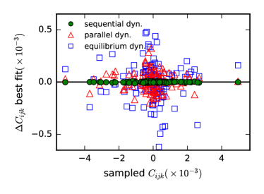
Figure 2: Distinguishing different dynamical models on the basis of three-point correlations. We sample configurations from the NESS of Glauber dynamics with sequential updates, see text. Next, we reconstruct the model parameters from the magnetisations, two- and three-point correlations, assuming the data was generated by Glauber dynamics with sequential updates (circles), parallel updates (triangles), or equilibrium dynamics (squares). The deviations $\Delta C_{ijk}=C_{ijk}(\mathbf{h},\boldsymbol{J})-C_{ijk}^{\text{sampled}}$ of the three-point correlations predicted by these three models from the corresponding correlations seen in the original samples are plotted against the sampled correlations. The relative root-mean-squared prediction errors $\|\Delta C_{ijk}\|_{2}/\|C_{ijk}^{\text{sampled}}\|_{2}$ are $0.003$, $0.06$, and $0.13$ for the sequential, parallel, and equilibrium dynamics respectively, clearly favouring the dynamics with sequential updates. The horizontal line is a guide to the eye representing a perfect fit. We used $N=10$ spins, a coupling and external field strength of $\beta=0.2$ and $M=10^{10}N$ samples.

The inverse Langevin problem.

Our approach is not limited to the asymmetric Ising problem with its binary spins and discrete-time dynamics. Consider the dynamics of continuous variables $x_{i}$ under a model of the form

$$\partial_{t}x_{i}=f(\theta_{i})-x_{i}+\xi_{i}(t)\ ,$$ (10)

where the effective local field is $\theta_{i}(t)=h_{i}+\sum_{j}J_{ij}x_{j}(t)$, $f(\theta)$ is an arbitrary monotonic function, and $\xi_{i}(t)$ describes $\delta$-correlated white noise. This is a multivariate Langevin equation; the steady state, if it exists, generally does not obey detailed balance. For the particular choice $f(\theta)=\tanh(\theta)$, this Langevin equation has magnetisations and correlations given by (3) and (4), and these results can be generalised easily to arbitrary choices of $f(\theta)$. Hence these equations and their generalisations can also be used to solve the inverse problem for the class of non-equilibrium stochastic differential equations of the form (10).

To conclude, we have used a self-consistent characterisation of the non-equilibrium steady state for the inference of model parameters from independent samples, that is, without direct recourse to the dynamics of the system. We showed that in the case of the asymmetric Ising model, correlations beyond two-point correlation are necessary for parameter inference, and that three-point correlations are in fact sufficient for this task.

References

- Cocco et al. (2009) S. Cocco, S. Leibler, and R. Monasson, Proc. Natl. Acad. Sci. USA 106, 14058 (2009).
- D’haeseleer et al. (2000) P. D’haeseleer, S. Liang, and R. Somogyi, Bioinformatics 16, 707 (2000).
- Weigt et al. (2009) M. Weigt, R. A. White, H. Szurmant, J. A. Hoch, and T. Hwa, Proc. Natl. Acad. Sci. USA 106, 67 (2009).
- (4) T. Mora, A. M. Walczak, W. Bialek, and C. G. Callan, Proc. Natl. Acad. Sci. USA 107, 5405 (2010), K. Shekhar et al. Phys. Rev. E 88, 062705 (2013).
- Bialek et al. (2012) W. Bialek et al. Proc. Natl. Acad. Sci. USA 109, 4786 (2012).
- (6) H. J. Kappen and F. B. Rodríguez, Neural Comput. 10, 1137 (1998) , V. Sessak and R. Monasson, J. Phys. A: Math. Theor. 42, 055001 (2009) , S. Cocco and R. Monasson, Phys. Rev. Lett. 106, 090601 (2011) , P. Ravikumar, M. J. Wainwright, and J. D. Lafferty, Ann. Stat. 38, 1287 (2010) , E. Aurell and M. Ekeberg, Phys. Rev. Lett. 108, 090201 (2012) , H. C. Nguyen and J. Berg, Phys. Rev. Lett. 109, 050602 (2012).
- Glauber (1963) R. J. Glauber, Journal of Mathematical Physics 4, 294 (1963).
- Derrida et al. (1987) B. Derrida, E. Gardner, and A. Zippelius, Europhys. Lett. 4, 167 (1987).
- Bailly-Bechet et al. (2010) M. Bailly-Bechet, A. Braunstein, A. Pagnani, M. Weigt, and R. Zecchina, BMC Bioinformatics 11, 355 (2010).
- Roudi and Hertz (2011) Y. Roudi and J. Hertz, Phys. Rev. Lett. 106, 048702 (2011).
- Zeng et al. (2013) H.-L. Zeng, M. Alava, E. Aurell, J. Hertz, and Y. Roudi, Phys. Rev. Lett. 110, 210601 (2013).
- Mézard and Sakellariou (2011) M. Mézard and J. Sakellariou, J. Stat. Mech. , L07001 (2011).
- Ackley et al. (1985) D. H. Ackley, G. E. Hinton, and T. J. Sejnowski, Cognitive Science 9, 147 (1985).
- Kappen and Spanjers (2000) H. J. Kappen and J. J. Spanjers, Phys. Rev. E 61, 5658 (2000).