$b\to ss{\bar{d}}$ decay in Randall-Sundrum models

Abstract

The extremely small branching ratio of $b\to ss{\bar{d}}$ decay in the Standard Model makes it a suitable channel to explore new-physics signals. We study this $\Delta S=2$ process in Randall-Sundrum models, including the custodially protected and the bulk-Higgs Randall-Sundrum models. Exploring the experimentally favored parameter spaces of these models, it suggests a possible enhancement of the decay rate, compared to the Standard Model result, by at most two orders of magnitude.

1 Introduction

In studying flavor-changing neutral-current (FCNC) transitions in rare B decays for exploring new physics (NP), one major difficulty is, how to reliably subtract the Standard Model (SM) background. Theoretical uncertainties in FCNC transitions make it hard to conclude about definite new physics signals against SM predictions. For this reason, an alternative approach suggested in [1, 2] is to consider processes which have tiny strengths in SM so that mere detection of such processes will indicate NP. One such process is the rare $b\to ss{\bar{d}}$ decay, as reported in [1, 2], which can serve the purpose of exposing NP.

The $\Delta S=2$ $b\to ss{\bar{d}}$ process is box mediated in SM and is found to occur with a branching ratio of the order of $10^{-12}$. The authors of Ref. [1] suggested $B^{-}\to K^{-}K^{-}\pi^{+}$ as the most appropriate mode for experimental searches and many other studies of the $b\to ss{\bar{d}}$ decay have been conducted in various beyond SM scenarios [3, 4, 5]. The first search was reported in [6] and upper limits were given by both B factories [7, 8, 9], with the current upper limit reported by BABAR Collaboration to be $\mathcal{B}(B^{-}\to K^{-}K^{-}\pi^{+})<1.6\times 10^{-7}$. Moreover, two-body exclusive decays of $B^{-}$ [10] and $B_{c}$ [11], which are driven by the $b\to ss{\bar{d}}$ transition, have also been studied in SM and in various extensions of it.

In this paper, we consider the inclusive $b\to ss{\bar{d}}$ decay in Randall-Sundrum (RS) models [12, 13]. We shall study two models known as the RS model with custodial protection $(\text{RS}_{c})$ [14, 15, 16, 17, 18] and the bulk-Higgs RS model [19, 20], in both of which FCNC transitions occur at tree level.

2 RS model with custodial protection

$\text{RS}_{c}$ model is based on a single warped extra-dimension with the bulk gauge group $\text{SU}(3)_{c}\times\text{SU}(2)_{L}\times\text{SU}(2)_{R}\times\text{U}(1)_{X}\times P_{LR}$. In the $\text{RS}_{c}$ model, the $\Delta S=2$ $b\to ss{\bar{d}}$ decay receives tree level contributions from the Kaluza-Klein (KK) gluons, the heavy KK photons, new heavy electroweak (EW) gauge bosons $Z_{H}$ and $Z^{\prime}$, and in principle the $Z^{0}$ boson. Custodial protection of the $Zb_{L}{\bar{b}}_{L}$ coupling through the discrete $P_{LR}$ symmetry in order to satisfy EW precision constraints render tree-level $Z^{0}$ contributions to be negligible. It was pointed out in [21] that for the $\text{RS}_{c}$ model the $\Delta F=2$ contributions from Higgs boson exchange are of $\mathcal{O}(v^{4}/{M_{\text{KK}}}^{4})$ ($v\approx$ 246 GeV is the Higgs vacuum expectation value and $M_{\mathrm{KK}}$ is the KK scale always larger than 1 TeV) and the importance of Higgs FCNCs is limited with the most pronounced effects occurring in the case of the CP-violating parameter $\epsilon_{K}$, but even there they are typically smaller than the corrections due to KK-gluon exchanges [22]. Therefore, in view of the possible Higgs-boson effects to be insignificant in $\Delta F=2$ processes, we simply neglect them in our study of the $b\to ss{\bar{d}}$ decay in the $\text{RS}_{c}$ model.

For the $\text{RS}_{c}$ model, we consider only first KK excitations of gauge bosons with $M_{\text{KK}}$ setting the mass scale for the low-lying KK excitations of the SM particles such that the mass of the first KK bosons are given by $M_{g^{(1)}}\approx 2.45$ $M_{\text{KK}}$. Here it is important to mention that we have used a different notation for the mass of the first KK gluon than in [23], our $M_{\text{KK}}$ corresponds to their $f$. The dominant contribution comes from the KK gluon, while the new heavy EW gauge bosons $(Z_{H},Z^{\prime})$ can compete with it. The tree-level $Z^{0}$ and KK photon contributions are very small. The effective Hamiltonian for the $\Delta S=2$ $b\to ss{\bar{d}}$ decay mediated by exchanges of the lightest KK gluon, the lightest KK photon and $(Z_{H},Z^{\prime})$ with the Wilson coefficients corresponding to $\mu=\mathcal{O}(M_{g^{(1)}})$ is given by

$$[\mathcal{H}_{\text{eff}}^{\Delta S=2}]_{\text{KK}} =\frac{1}{2(M_{g^{(1)}})^{2}}[C_{1}^{VLL}\mathcal{Q}_{1}^{VLL}+C_{1}^{VRR}\mathcal{Q}_{1}^{VRR}$$

$$+C_{1}^{LR}\mathcal{Q}_{1}^{LR}+C_{2}^{LR}\mathcal{Q}_{2}^{LR}+C_{1}^{RL}\mathcal{Q}_{1}^{RL}+C_{2}^{RL}\mathcal{Q}_{2}^{RL}],$$ (1)

where

$$\mathcal{Q}_{1}^{VLL} =(\bar{s}\gamma_{\mu}P_{L}b)(\bar{s}\gamma^{\mu}P_{L}d),$$

$$\mathcal{Q}_{1}^{VRR} =(\bar{s}\gamma_{\mu}P_{R}b)(\bar{s}\gamma^{\mu}P_{R}d),$$

$$\mathcal{Q}_{1}^{LR} =(\bar{s}\gamma_{\mu}P_{L}b)(\bar{s}\gamma^{\mu}P_{R}d),$$

$$\mathcal{Q}_{2}^{LR} =(\bar{s}P_{L}b)(\bar{s}P_{R}d),$$

$$\mathcal{Q}_{1}^{RL} =(\bar{s}\gamma_{\mu}P_{R}b)(\bar{s}\gamma^{\mu}P_{L}d),$$

$$\mathcal{Q}_{2}^{RL} =(\bar{s}P_{R}b)(\bar{s}P_{L}d),$$ (2)

and

$$C_{i}^{j}(M_{g^{(1)}}) =[C_{i}^{j}(M_{g^{(1)}})]^{G}+[\Delta C_{i}^{j}(M_{g^{(1)}})]^{\text{QED}}+[\Delta C_{i}^{j}(M_{g^{(1)}})]^{\text{EW}},$$ (3)

with $i=1,2$ and $j=VLL,VRR,LR,RL$. Note that, in the $\text{RS}_{c}$ model, compared to the analogous processes $K^{0}-\bar{K}^{0}$ and $B_{s}^{0}-\bar{B}_{s}^{0}$ mixings [23], the $b\to ss{\bar{d}}$ decay receives additional contributions from the $RL$ operators. $[C_{i}^{j}(M_{g^{(1)}})]^{G}$ in Eq. (3) denote the contributions from the KK gluon to the Wilson coefficients that are calculated to be

$$[C_{1}^{VLL}(M_{g^{(1)}})]^{G}=\frac{2}{3}{p_{\text{UV}}}^{2}\Delta_{L}^{sb}\Delta_{L}^{sd},$$

$$[C_{1}^{VRR}(M_{g^{(1)}})]^{G}=\frac{2}{3}{p_{\text{UV}}}^{2}\Delta_{R}^{sb}\Delta_{R}^{sd},$$

$$[C_{1}^{LR}(M_{g^{(1)}})]^{G}=-\frac{1}{3}{p_{\text{UV}}}^{2}\Delta_{L}^{sb}\Delta_{R}^{sd},$$

$$[C_{2}^{LR}(M_{g^{(1)}})]^{G}=-2{p_{\text{UV}}}^{2}\Delta_{L}^{sb}\Delta_{R}^{sd},$$

$$[C_{1}^{RL}(M_{g^{(1)}})]^{G}=-\frac{1}{3}{p_{\text{UV}}}^{2}\Delta_{R}^{sb}\Delta_{L}^{sd},$$

$$[C_{2}^{RL}(M_{g^{(1)}})]^{G}=-2{p_{\text{UV}}}^{2}\Delta_{R}^{sb}\Delta_{L}^{sd},$$ (4)

where, $p_{\text{UV}}$ parameterizes the influence of brane kinetic terms on the $\text{SU}(3)_{c}$ coupling. In our analysis we set $p_{\text{UV}}\equiv 1$. Similarly, for the KK photon and $(Z_{H},Z^{\prime})$ contributions, we find the following corrections to the Wilson coefficients $C_{i}^{j}(M_{g^{(1)}})$,

$$[\Delta C_{1}^{VLL}(M_{g^{(1)}})]^{\text{QED}} =2[\Delta_{L}^{sb}(A^{(1)})][\Delta_{L}^{sd}(A^{(1)})],$$

$$[\Delta C_{1}^{VRR}(M_{g^{(1)}})]^{\text{QED}} =2[\Delta_{R}^{sb}(A^{(1)})][\Delta_{R}^{sd}(A^{(1)})],$$

$$[\Delta C_{1}^{LR}(M_{g^{(1)}})]^{\text{QED}} =2[\Delta_{L}^{sb}(A^{(1)})][\Delta_{R}^{sd}(A^{(1)})],$$

$$[\Delta C_{2}^{LR}(M_{g^{(1)}})]^{\text{QED}} =0,$$

$$[\Delta C_{1}^{RL}(M_{g^{(1)}})]^{\text{QED}} =2[\Delta_{R}^{sb}(A^{(1)})][\Delta_{L}^{sd}(A^{(1)})],$$

$$[\Delta C_{2}^{RL}(M_{g^{(1)}})]^{\text{QED}} =0,$$ (5)

$$[\Delta C_{1}^{VLL}(M_{g^{(1)}})]^{\text{EW}} =2[\Delta_{L}^{sb}(Z^{(1)})\Delta_{L}^{sd}(Z^{(1)})+\Delta_{L}^{sb}(Z_{X}^{(1)})\Delta_{L}^{sd}(Z_{X}^{(1)})],$$

$$[\Delta C_{1}^{VRR}(M_{g^{(1)}})]^{\text{EW}} =2[\Delta_{R}^{sb}(Z^{(1)})\Delta_{R}^{sd}(Z^{(1)})+\Delta_{R}^{sb}(Z_{X}^{(1)})\Delta_{R}^{sd}(Z_{X}^{(1)})],$$

$$[\Delta C_{1}^{LR}(M_{g^{(1)}})]^{\text{EW}} =2[\Delta_{L}^{sb}(Z^{(1)})\Delta_{R}^{sd}(Z^{(1)})+\Delta_{L}^{sb}(Z_{X}^{(1)})\Delta_{R}^{sd}(Z_{X}^{(1)})],$$

$$[\Delta C_{2}^{LR}(M_{g^{(1)}})]^{\text{EW}} =0,$$

$$[\Delta C_{1}^{RL}(M_{g^{(1)}})]^{\text{EW}} =2[\Delta_{R}^{sb}(Z^{(1)})\Delta_{L}^{sd}(Z^{(1)})+\Delta_{R}^{sb}(Z_{X}^{(1)})\Delta_{L}^{sd}(Z_{X}^{(1)})],$$

$$[\Delta C_{2}^{RL}(M_{g^{(1)}})]^{\text{EW}} =0,$$ (6)

where the overlap integrals $\Delta_{L,R}^{sb}(Z^{(1)})$, $\Delta_{L,R}^{sb}(Z_{X}^{(1)})$, $\Delta_{L,R}^{sd}(Z^{(1)})$ and $\Delta_{L,R}^{sd}(Z_{X}^{(1)})$ are given in Appendix B of [23]. These overlap integrals contain the profiles of the zero mode fermions and shape functions of the KK gauge bosons. We estimate the size of EW contributions compared to the KK gluon contributions in the $b\to ss{\bar{d}}$ decay by factoring out all the couplings and charge factors from $\Delta_{L,R}^{sb}$ and $\Delta_{L,R}^{sd}$. The remaining $\tilde{\Delta}_{L,R}^{sb}$ and $\tilde{\Delta}_{L,R}^{sd}$ are then universal for all the gauge bosons considered up to the different boundary conditions. Combining contributions in Eqs. (2), (2) and (2) and evaluating the various couplings, we have

$$C_{1}^{VLL}(M_{g^{(1)}})=[0.67+0.02+0.56]\tilde{\Delta}_{L}^{sb}\tilde{\Delta}_{L}^{sd}=1.25\tilde{\Delta}_{L}^{sb}\tilde{\Delta}_{L}^{sd},$$

$$C_{1}^{VRR}(M_{g^{(1)}})=[0.67+0.02+0.98]\tilde{\Delta}_{R}^{sb}\tilde{\Delta}_{R}^{sd}=1.67\tilde{\Delta}_{R}^{sb}\tilde{\Delta}_{R}^{sd},$$

$$C_{1}^{LR}(M_{g^{(1)}})=[-0.333+0.02+0.56]\tilde{\Delta}_{L}^{sb}\tilde{\Delta}_{R}^{sd}=0.25\tilde{\Delta}_{L}^{sb}\tilde{\Delta}_{R}^{sd},$$

$$C_{1}^{RL}(M_{g^{(1)}})=[-0.333+0.02+0.56]\tilde{\Delta}_{R}^{sb}\tilde{\Delta}_{L}^{sd}=0.25\tilde{\Delta}_{R}^{sb}\tilde{\Delta}_{L}^{sd},$$ (7)

where the three contributions in the bracket correspond to the KK gluon, the KK photon and combined $(Z_{H},Z^{\prime})$ exchange, respectively. The Wilson coefficients $C_{2}^{LR}(M_{g^{(1)}})$ and $C_{2}^{RL}(M_{g^{(1)}})$ receive only the KK-gluon contributions. We see that the EW contributions, dominated by $(Z_{H},Z^{\prime})$ exchanges, give +87$\%$ and +150$\%$ corrections in the case of $C_{1}^{VLL}(M_{g^{(1)}})$ and $C_{1}^{VRR}(M_{g^{(1)}})$, respectively, while corrections of $-$174$\%$ are observed for $C_{1}^{LR}(M_{g^{(1)}})$ and $C_{1}^{RL}(M_{g^{(1)}})$. The Hamiltonian in Eq. (2) is valid at scales of $\mathcal{O}(M_{g^{(1)}})$ and has to be evolved to a low energy scale $\mu_{b}$ = 4.6 GeV. For that, the anomalous dimension matrices for $\Delta F=2$ four-quark dimension-six operators have already been calculated at two loop level in [24, 25]. As gluons are flavor blind and QCD preserves chirality so the anomalous dimension matrices of the operators in $b\to ss{\bar{d}}$ are the same as for the case of $B_{d,s}^{0}-\bar{B}_{d,s}^{0}$ mixing operators. Therefore, the renormalization group running of the Wilson coefficients for the $b\to ss{\bar{d}}$ decay is performed by using analytic formulae for the relevant QCD factors given in Section 3.1 and appendix C of [26]. Finally, the decay width for the $b\to ss{\bar{d}}$ decay in the $\text{RS}_{c}$ model is given by

$${\it\Gamma} =\frac{m_{b}^{5}}{3072(2\pi)^{3}(M_{g^{(1)}})^{4}}[16(|C_{1}^{VLL}(\mu_{b})|^{2}+|C_{1}^{VRR}(\mu_{b})|^{2})$$

$$+12(|C_{1}^{LR}(\mu_{b})|^{2}+|C_{1}^{RL}(\mu_{b})|^{2})+3(|C_{2}^{LR}(\mu_{b})|^{2}+|C_{2}^{RL}(\mu_{b})|^{2})$$

$$-2\mathcal{R}e(C_{1}^{LR}(\mu_{b})C_{2}^{*LR}(\mu_{b})+C_{2}^{LR}(\mu_{b})C_{1}^{*LR}(\mu_{b})$$

$$+C_{1}^{RL}(\mu_{b})C_{2}^{*RL}(\mu_{b})+C_{2}^{RL}(\mu_{b})C_{1}^{*RL}(\mu_{b}))].$$ (8)

3 Bulk-Higgs RS model

The bulk-Higgs RS model is based on the 5D gauge group $\text{SU}(3)_{c}\times\text{SU}(2)_{V}\times\text{U}(1)_{Y}$, where all the fields are allowed to propagate in the 5D space-time [20]. $b\to ss{\bar{d}}$ decay in the bulk-Higgs RS model results from tree-level exchanges of Kaluza-Klein gluons and photons, the $Z^{0}$ boson and the Higgs boson as well as their KK excitations and the extended scalar fields $\phi^{Z(n)}$. For the bulk-Higgs RS model we consider the summation over the contributions from the entire KK towers, with the lightest KK states having mass $M_{g^{(1)}}\approx 2.45$ $M_{\text{KK}}$. We start with the effective NP Hamiltonian

$$[\mathcal{H}_{\text{eff}}^{\Delta S=2}]_{\text{KK}} =\sum_{n=1}^{5}[C_{n}\mathcal{O}_{n}+\tilde{C}_{n}\tilde{\mathcal{O}}_{n}],$$ (9)

where

$$\mathcal{O}_{1} =(\bar{s}_{L}\gamma_{\mu}b_{L})(\bar{s}_{L}\gamma^{\mu}d_{L}),$$

$$\mathcal{O}_{2} =(\bar{s}_{R}b_{L})(\bar{s}_{R}d_{L}),$$

$$\mathcal{O}_{3} =(\bar{s}_{R}^{\alpha}b_{L}^{\beta})(\bar{s}_{R}^{\beta}d_{L}^{\alpha}),$$

$$\mathcal{O}_{4} =(\bar{s}_{R}b_{L})(\bar{s}_{L}d_{R}),$$

$$\mathcal{O}_{5} =(\bar{s}_{R}^{\alpha}b_{L}^{\beta})(\bar{s}_{L}^{\beta}d_{R}^{\alpha}).$$ (10)

A summation over color indices $\alpha$ and $\beta$ is understood. The $\tilde{O}_{n}$ operators are obtained from $O_{n}$ by $L\leftrightarrow R$ exchange. Wilson coefficients at $\mathcal{O}(M_{\text{KK}})$ are given by

$$C_{1} =\frac{4\pi L}{M_{\text{KK}}^{2}}(\tilde{\Delta}_{D})_{23}\otimes(\tilde{\Delta}_{D})_{21}[\frac{\alpha_{s}}{2}(1-\frac{1}{N_{c}})+\alpha Q_{d}^{2}+\frac{\alpha}{s_{w}^{2}c_{w}^{2}}(T_{3}^{d}-Q_{d}s_{w}^{2})^{2}],$$

$$\tilde{C}_{1} =\frac{4\pi L}{M_{\text{KK}}^{2}}(\tilde{\Delta}_{d})_{23}\otimes(\tilde{\Delta}_{d})_{21}[\frac{\alpha_{s}}{2}(1-\frac{1}{N_{c}})+\alpha Q_{d}^{2}+\frac{\alpha}{s_{w}^{2}c_{w}^{2}}(-Q_{d}s_{w}^{2})^{2}],$$

$$C_{4} =-\frac{4\pi L\alpha_{s}}{M_{\text{KK}}^{2}}(\tilde{\Delta}_{D})_{23}\otimes(\tilde{\Delta}_{d})_{21}-\frac{L}{\pi\beta M_{\text{KK}}^{2}}(\tilde{\Omega}_{d})_{23}\otimes(\tilde{\Omega}_{D})_{21},$$

$$\tilde{C}_{4} =-\frac{4\pi L\alpha_{s}}{M_{\text{KK}}^{2}}(\tilde{\Delta}_{d})_{23}\otimes(\tilde{\Delta}_{D})_{21}-\frac{L}{\pi\beta M_{\text{KK}}^{2}}(\tilde{\Omega}_{D})_{23}\otimes(\tilde{\Omega}_{d})_{21},$$

$$C_{5} =\frac{4\pi L}{M_{\text{KK}}^{2}}(\tilde{\Delta}_{D})_{23}\otimes(\tilde{\Delta}_{d})_{21}[\frac{\alpha_{s}}{N_{c}}-2\alpha Q_{d}^{2}+\frac{2\alpha}{s_{w}^{2}c_{w}^{2}}(T_{3}^{d}-Q_{d}s_{w}^{2})(Q_{d}s_{w}^{2})],$$

$$\tilde{C}_{5} =\frac{4\pi L}{M_{\text{KK}}^{2}}(\tilde{\Delta}_{d})_{23}\otimes(\tilde{\Delta}_{D})_{21}[\frac{\alpha_{s}}{N_{c}}-2\alpha Q_{d}^{2}+\frac{2\alpha}{s_{w}^{2}c_{w}^{2}}(T_{3}^{d}-Q_{d}s_{w}^{2})(Q_{d}s_{w}^{2})],$$ (11)

where $Q_{d}=-1/3$, $T_{3}^{d}=-1/2$, and $N_{c}=3$. Higgs and scalar field $\phi^{Z}$ give opposite contributions to the Wilson coefficient $C_{2}$, thus they cancel each other giving $C_{2}=0$. Similarly, $\tilde{C}_{2}=0$. The expressions of the mixing matrices $(\tilde{\Delta}_{F(f)})_{mn}\otimes(\tilde{\Delta}_{F(f)})_{m^{\prime}n^{\prime}}$ and $(\tilde{\Omega}_{F(f)})_{mn}\otimes(\tilde{\Omega}_{F(f)})_{m^{\prime}n^{\prime}}$ (with $F=U,D$ and $f=u,d,$ and similarly in the lepton sector) in terms of the overlap integrals of boson and fermion profiles in the bulk-Higgs RS model, will be reported in [19]. For the present study, we restrict ourselves to the $3\times 3$ submatrices governing the couplings of the SM fermion fields. In the zero mode approximation (ZMA), the required expressions are simplified considerably with (see also [27])

$$(\tilde{\Delta}_{D})_{23}\otimes(\tilde{\Delta}_{d})_{21} \rightarrow(U_{d}^{\dagger})_{2i}(U_{d})_{i3}(\tilde{\Delta}_{Dd})_{ij}(W_{d}^{\dagger})_{2j}(W_{d})_{j1},$$

$$(\tilde{\Delta}_{Dd})_{ij} =\frac{F^{2}(c_{Q_{i}})}{3+2c_{Q_{i}}}\frac{3+c_{Q_{i}}+c_{d_{j}}}{2(2+c_{Q_{i}}+c_{d_{j}})}\frac{F^{2}(c_{d_{j}})}{3+2c_{d_{j}}},$$

$$(\tilde{\Omega}_{D})_{23}\otimes(\tilde{\Omega}_{d})_{21} \rightarrow(U_{d}^{\dagger})_{2i}(W_{d})_{j3}(\tilde{\Omega}_{Dd})_{ijkl}(W_{d}^{\dagger})_{2k}(U_{d})_{l1},$$

$$(\tilde{\Omega}_{Dd})_{ijkl}= \frac{\pi(1+\beta)}{4L}\frac{F(c_{Q_{i}})F(c_{d_{j}})}{2+\beta+c_{Q_{i}}+c_{d_{j}}}$$

$$\times\frac{(Y_{d})_{ij}(Y_{d}^{\dagger})_{kl}(4+2\beta+c_{Q_{i}}+c_{d_{j}}+c_{d_{k}}+c_{Q_{l}})}{4+c_{Q_{i}}+c_{d_{j}}+c_{d_{k}}+c_{Q_{l}}}$$

$$\times\frac{F(c_{d_{k}})F(c_{Q_{l}})}{2+\beta+c_{d_{k}}+c_{Q_{l}}},$$

where $U_{d}$ and $W_{d}$ are flavor matrices diagonalising the SM down-type Yukawa matrix. $\beta$ is a parameter of the model related to the Higgs profile and $c^{\prime}s$ are bulk-mass parameters of fermions, which control the localization of fermions in the warped extra dimension. The 5D Yukawa matrix $Y_{d}$ has anarchic $\mathcal{O}(1)$ complex elements, which together with other flavor parameters generate the right quark masses. Summation over indices $i,j,k$ and $l$ is understood. Analogous expressions hold for remaining combinations of $D$ and $d$. The Effective Hamiltonian given in Eq. (9) is valid at $\mathcal{O}(M_{\text{KK}})$, which must be evolved to a low-energy scale $\mu_{b}$. Hence for the evolution of the Wilson coefficients we use the formulae of NLO QCD factors given in [28]. After that, the decay width in the bulk-Higgs RS model is given by

$${\it\Gamma} =\frac{m_{b}^{5}}{3072(2\pi)^{3}}[64(|C_{1}(\mu_{b})|^{2}+|\tilde{C}_{1}(\mu_{b})|^{2})$$

$$+12(|C_{4}(\mu_{b})|^{2}+|\tilde{C}_{4}(\mu_{b})|^{2}+|C_{5}(\mu_{b})|^{2}+|\tilde{C}_{5}(\mu_{b})|^{2})$$

$$+4\mathcal{R}e(C_{4}(\mu_{b})C_{5}^{*}(\mu_{b})+C_{4}^{*}(\mu_{b})C_{5}(\mu_{b})$$

$$+\tilde{C}_{4}(\mu_{b})\tilde{C}_{5}^{*}(\mu_{b})+\tilde{C}_{4}^{*}(\mu_{b})\tilde{C}_{5}(\mu_{b}))].$$ (12)

4 Phenomenological bounds on RS models

In this section we discuss the relevant constraints on the parameter spaces of the RS models coming from the EW precision tests and the latest measurements of the Higgs signal strengths at the LHC. In addition, we will also consider the constraints coming from $K^{0}-\bar{K}^{0}$ and $B_{s}^{0}-\bar{B}_{s}^{0}$ mixing in Section 5.

First, considering the $\text{RS}_{c}$ model, the bounds induced from EW precision tests allow for KK masses in the few TeV range. A recent tree-level analysis of the S and T parameters yields $M_{g^{(1)}}>4.8$ TeV at $95\%$ confidence level (CL) for the mass of the lightest KK gluon and photon resonances [29]. While comparing the predictions of the signal rates for the various Higgs-boson decays with the latest data from the LHC, it is suggested in [30] that the most stringent bounds emerge from the signal rates for $pp\rightarrow h\rightarrow ZZ^{\ast},WW^{\ast}$. In the RS_c model, KK gluon masses lighter than $22.7$ $\text{TeV}\times(y_{\star}/3)$ in the brane-Higgs case and $13.2$ $\text{TeV}\times(y_{\star}/3)$ in the narrow bulk-Higgs scenario are excluded at $95\%$ CL, where the $y_{\star}=\mathcal{O}(1)$ is a free parameter and is defined as the upper bound on the various entries of the Yukawa matrices that are taken to be complex random numbers such that $|(Y_{f})_{ij}|\leq y_{\star}$. Thus, for $y_{\star}=3$ the bounds derived from Higgs physics are much stronger than those stemming from EW precision measurements. In order to lower these bounds, smaller values of $y_{\star}$ can be considered. For that it was also presented in Ref. [30] that for the lowest value of the lightest KK gluon mass $M_{g^{(1)}}=4.8$ TeV implied by EW precision constraints, in the RS_c model, the constraints at $95\%$ CL on the values of the $y_{\star}$ are given by $y_{\star}<0.3$ for the brane-Higgs scenario, and $y_{\star}<1.1$ for the narrow bulk-Higgs case. However, realizing the fact that too small Yukawa couplings would give rise to enhanced corrections to $\epsilon_{K}$ and hence they would reinforce the RS flavor problem, relatively loose bound on the values of the $y_{\star}$ can be obtained for the lightest KK gluon mass of $M_{g^{(1)}}=10$ TeV. For instance, in the $\text{RS}_{c}$ model, the constraints on the value of $y_{\star}$ at $95\%$ CL valid for $M_{g^{(1)}}=10$ TeV are given by $y_{\star}<1.1$ and $y_{\star}<2.25$ for the brane-Higgs case and the narrow bulk-Higgs case, respectively [30].

Next, we consider the bulk-Higgs RS model. The constraints on the KK mass scale in the bulk-Higgs RS model implied by the analyses of EW precision data are given in [20]. Under a constrained fit (i.e. $U=0$), the obtained lower bounds on the KK mass scale at $95\%$ CL vary between $M_{\text{KK}}>3.0$ TeV for $\beta=0$ to $M_{\text{KK}}>5.1$ TeV for $\beta=10$. With an unconstrained fit, these bounds relax to $M_{\text{KK}}>2.5$ TeV and $M_{\text{KK}}>4.3$ TeV, respectively. For significantly larger values of $\beta$, the lower bounds increase towards the brane localized Higgs limit.

Table 1: Default values of the input parameters used in the SM calculation [31].

$G_{F}=1.16637\times 10^{-5}$ GeV-2, $m_{b}=4.66_{-0.03}^{+0.04}$ GeV,

$m_{c}=1.27\pm 0.03$ GeV, $m_{t}=173.21\pm 0.51$ GeV, $m_{W}=80.385\pm 0.015$ GeV,

$\tau_{B}=(1.566\pm 0.003)\times 10^{-12}$ sec, $\sin{2\beta}=0.691\pm 0.017$,

$|V_{tb}V_{ts}^{\ast}|=(40\pm 2)\times 10^{-3}$, $|V_{td}V_{ts}^{\ast}|=(32\pm 3)\times 10^{-5}$, $|V_{cd}V_{cs}^{\ast}|=(21.8\pm 0.6)\times 10^{-2}$.

5 Numerical analysis

In this section we present the results of the $b\to ss{\bar{d}}$ decay rate in RS models. Before proceeding to analyze the NP, we first estimate the size of the leading order SM result. The numerical values of the parameters that are involved in the SM calculation are listed in table 1. Employing the formula of the SM $b\to ss{\bar{d}}$ decay rate [2], we get

$$\mathcal{B}(b\to ss{\bar{d}})_{\text{SM}}=(2.19\pm 0.38)\times 10^{-12}.$$ (13)

Next, we explore the parameter space of the $\text{RS}_{c}$ model by the strategy outlined in [23]. It was pointed out in [23] that there exist regions in parameter space, without much fine-tuning in the 5D Yukawa couplings, which satisfy all existing $\Delta F=2$ and EW precision constraints for scales of masses of lightest KK gauge bosons $M_{\text{KK}}\simeq$ 3 TeV. However, as mentioned above that for the anarchic Yukawa couplings with $y_{\star}=3$ in the $\text{RS}_{c}$ model with the a brane Higgs, the constraints on $M_{g^{(1)}}$ emerging from Higgs physics, are much stronger than the EW precision constraints, so in our study of the $\text{RS}_{c}$ model, we generate two sets of fundamental 5D Yukawa matrices with $y_{\star}=1.5$ and $3$. For the first set the 28 parameters contained in the fundamental 5D Yukawa matrices are randomly chosen in their respective ranges, $[0,\pi/2]$, $[0,2\pi]$ and $[0.1,1.5]$ for angles, phases and $|(Y_{f})_{ij}|$, respectively. Whereas, in the second set $|(Y_{f})_{ij}|$ are chosen randomly in the range $[0.1,3]$, by keeping ranges for angles and phases same as previously. In order to determine the nine quark bulk-mass parameters $c_{Q,u,d}^{i}$, we take $0.4\leq c_{Q}^{3}\leq 0.45$ in our scan, allowing for consistency with EW precision data, so that the remaining bulk mass parameters are determined making use of the analytic formulae presented in section 3 of [23]. Finally, by diagonalising numerically the obtained effective 4D Yukawa coupling matrices, we keep only those parameter sets that in addition to the quark masses and CKM mixing angles also reproduce the proper value of the Jarlskog determinant, all within their respective $2\sigma$ ranges. The flavor transitions that would be involved in the $b\to ss{\bar{d}}$ mode will commonly also give contributions to $K^{0}-\bar{K}^{0}$ and $B_{s}^{0}-\bar{B}_{s}^{0}$ mixings, so we consider $\Delta M_{K}$, $\epsilon_{K}$ and $\Delta M_{B_{s}}$ constraints on the parameter space in addition to EW precision constraints and the Higgs constraints mentioned above. Expressions of $(M_{12}^{K})_{\text{KK}}$ and $(M_{12}^{s})_{\text{KK}}$ relevant for $K^{0}-\bar{K}^{0}$ and $B_{s}^{0}-\bar{B}_{s}^{0}$ mixings constraints, calculated in the $\text{RS}_{c}$ model, are contained in Eqs. (4.32) and (4.33) of [23], respectively. Figure 1 shows the branching ratio of the RS_c predictions for the $b\to ss{\bar{d}}$ decay as a function of $M_{g^{(1)}}$ with two different values of $y_{\star}$. Note that we have excluded the SM contribution to display the decoupling behavior of the NP contribution as $M_{g^{(1)}}$ increases. The red and blue scatter points represent the cases of $y_{\star}=1.5$ and $3$, respectively. While imposing the experimental constraints for $\Delta M_{K}$, $\Delta M_{B_{s}}$ and $\epsilon_{K}$ in both cases, we set input parameters in table 2 to their central values and allow the resulting observables to deviate by $\pm 50\%$, $\pm 30\%$ and $\pm 30\%$, respectively. The predictions of the $b\to ss{\bar{d}}$ decay rates for the parameter points with $y_{\star}=1.5$ are generally larger than those with $y_{\star}=3$, but it can be seen in figure 1 that after applying the $\Delta M_{K}$, $\epsilon_{K}$ and $\Delta M_{B_{s}}$ constraints simultaneously, the maximum possible $y_{\star}=1.5$ prediction is reduced relatively close to that for the case of $y_{\star}=3$. However, after imposing the $K^{0}-\bar{K}^{0}$ and $B_{s}^{0}-\bar{B}_{s}^{0}$ mixings constraints, still for some parameter points with $y_{\star}=1.5$ in the low $M_{g^{(1)}}$ range, the branching ratio of $b\to ss{\bar{d}}$ decay in the $\text{RS}_{c}$ model can be close to the order of $10^{-10}$, which is approximately two orders of magnitude larger compared to the SM result. Considering the effects of the new heavy EW gauge bosons $Z_{H}$ and $Z^{\prime}$ in the $\text{RS}_{c}$ model, we found in agreement with [23] that while imposing the $\Delta M_{K}$ and $\epsilon_{K}$ constraints $Z_{H}$ and $Z^{\prime}$ give subleading contributions because the strong QCD renormalization group enhancement of the $C_{2}^{LR}$ coefficient and the chiral enhancement of the $\mathcal{Q}_{2}^{LR}$ hadronic matrix element in $(M_{12}^{K})_{\text{KK}}$ assure that the first KK gluon contributions still dominate over EW contributions. However, for the prediction of the branching ratio in the $b\to ss{\bar{d}}$ decay the QCD renormalization group enhancement in the $C_{2}^{LR}$ and $C_{2}^{RL}$ coefficients is smaller and the chiral enhancement is absent. Therefore, for a parameter point that satisfies the $\Delta M_{K}$, $\Delta M_{B_{s}}$ and $\epsilon_{K}$ constraints simultaneously, $Z_{H}$ and $Z^{\prime}$ increase the prediction of the branching ratio with comparable contributions to that of the first KK gluon.

Table 2: Values of experimental and theoretical quantities used as input parameters while scanning the parameter spaces of the RS models and in calculation of $\Delta M_{K}$, $\Delta M_{B_{s}}$ and $\epsilon_{K}$. Values of the parameters $B_{i}^{K}$ at $\mu_{L}=2$ GeV and $B_{i}^{s}$ at $\mu_{b}=4.6$ GeV are given in $\overline{\text{MS}}$-NDR scheme obtained for $K^{0}-\bar{K}^{0}$ and $B_{s}^{0}-\bar{B}_{s}^{0}$ mixings, respectively.

$|V_{us}|=0.226(2)$	$s_{w}^{2}=0.2312$
$|V_{ub}|=3.8(4)\times 10^{-3}$	$\alpha(m_{Z})=1/127.9$
$|V_{cb}|=4.1(1)\times 10^{-2}$ [32]	$\alpha_{s}(m_{Z})=0.1182\pm 0.0012$ [31]
$\lambda=0.2250\pm 0.0005$	$m_{K}=497.611$ MeV
$A=0.811\pm 0.026$	$m_{B_{s}}=5366.82$ MeV [31]
${\bar{\rho}}=0.124_{-0.018}^{+0.019}$	$\eta_{tt}=0.57\pm 0.01$ [33]
${\bar{\eta}}=0.356\pm 0.011$ [31]	$\eta_{cc}=1.50\pm 0.37$ [34]
$\Delta M_{K}=(3.484\pm 0.006)\times 10^{-15}$ GeV	$\eta_{ct}=0.47\pm 0.05$ [35, 36]
$\Delta M_{B_{s}}=(1.1688\pm 0.0014)\times 10^{-11}$ GeV	$\eta_{B}=0.55\pm 0.01$ [33]
$|\epsilon_{K}|=(2.228\pm 0.011)\times 10^{-3}$ [31]	$F_{K}=156$ MeV
$\phi_{\epsilon}=(43.52\pm 0.05)^{\circ}$ [31]	$F_{B_{s}}=245\pm 25$ MeV [37]
$\kappa_{\epsilon}=0.92\pm 0.02$ [38]
$\hat{B}_{K}=0.75$	$\mu_{L}=2$ GeV	$B_{1}^{K}=0.57,B_{4}^{K}=0.81,B_{5}^{K}=0.56$ [39]
$\hat{B}_{B_{s}}=1.22$ [37]	$\mu_{b}=4.6$ GeV	$B_{1}^{s}=0.87,B_{4}^{s}=1.16,B_{5}^{s}=1.75$ [40]

Figure 1: The branching ratio of $b\to ss{\bar{d}}$ as a function of the KK gluon mass $M_{g^{(1)}}$ in $\text{RS}_{c}$ model. The red and blue points correspond to $y_{\star}=1.5$ and $3$, respectively.

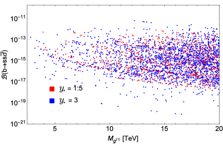
(a) $\beta$=1;

(b) $\beta$=10.

Figure 2: The branching ratio of $b\to ss{\bar{d}}$ as a function of the KK gluon mass $M_{g^{(1)}}$ in the bulk-Higgs RS model with $\beta=1$ and $\beta=10$. The red and blue scatter points correspond to $y_{\star}=1.5$ and $3$, respectively.

For the bulk-Higgs RS model, following the directions given in [20, 21], for a given value of $\beta$ and $M_{\text{KK}}$, we generate two sets of random and anarchic 5D Yukawa matrices, whose entries satisfy $|(Y_{u,d})_{ij}|\leq y_{\star}$ with $y_{\star}=1.5$ and 3. These values of $y_{\star}$ lie below the perturbativity bound, which is given by $y_{\star}<y_{\text{max}}$ with $y_{\text{max}}\sim 8.3/\sqrt{1+\beta}$ [20]. Moreover, for values of $y_{\star}<1$ it becomes increasingly difficult to fit the top-quark mass. Next, we require that the 5D Yukawa matrices with proper bulk-mass parameters $c_{Q_{i}}<1.5$ and $c_{q_{i}}<1.5$ reproduce the correct values for the SM quark masses evaluated at the scale $\mu=1$ TeV. In our analysis, we consider the two representative values $\beta=1$ and $\beta=10$ corresponding to broad Higgs profile and narrow Higgs profile, respectively. In figure 2, we show the NP predictions with $\beta=1$ and $10$, respectively, for the $b\to ss{\bar{d}}$ decay rate as a function of $M_{g^{(1)}}$, after simultaneously imposing the $\Delta M_{K}$, $\epsilon_{K}$ and $\Delta M_{B_{s}}$ constraints. The red and blue scatter points again correspond to model points obtained using $y_{\star}=1.5$ and 3, respectively. For the case of $y_{\star}=1.5$, the branching ratios are generally larger because of less suppressed FCNCs compared to $y_{\star}=3$ case, but as mentioned earlier the lower values of $y_{\star}$ are subject to more stringent constraints from flavour physics, so after imposing the $\Delta M_{K}$, $\epsilon_{K}$ and $\Delta M_{B_{s}}$ constraints, the maximum possible branching ratio of the parameter points with $y_{\star}=1.5$ in the bulk-Higgs RS model lies close to the SM result as shown in figure 2(a). While for the case of $y_{\star}=3$ in figure 2(a), subject to relatively less severe constraints from the $K^{0}-\bar{K}^{0}$ and $B_{s}^{0}-\bar{B}_{s}^{0}$ mixings compared with $y_{\star}=1.5$ case, the maximum possible branching ratio for some of the parameter points, even with suppressed FCNCs, lies close to the order $10^{-11}$. Situation is similar in the $\beta=10$ case, except that compared to the $\beta=1$ scenario, an order of magnitude enhancement for the maximum possible branching ratio is observed for both cases of $y_{\star}$, as displayed in figure 2(b).

6 Conclusions

We studied the $b\to ss{\bar{d}}$ decay in the $\text{RS}_{c}$ and the bulk-Higgs RS model. In both models, main contribution to the $b\to ss{\bar{d}}$ decay comes from tree level exchanges of KK gluons, while in the $\text{RS}_{c}$ model the contributions from the new heavy EW gauge bosons $Z_{H}$ and $Z^{\prime}$ can compete with the KK-gluon contributions. We employed renormalization group runnings of the Wilson coefficients with NLO QCD factors in both models. Although this decay receives tree level contributions, the parameter space is severely constrained by $K^{0}-\bar{K}^{0}$ mixing and $B_{s}^{0}-\bar{B}_{s}^{0}$ mixing experiments such that for broad Higgs profile corresponding to $\beta=1$ case no significant increase in the branching ratio is observed in the bulk-Higgs RS model compared to the SM result. Whereas, for the value $\beta=10$, it is possible to achieve an order of magnitude enhancement of the branching ratio for some of the parameter points. While, the $\text{RS}_{c}$ model with additional contributions from the new heavy EW gauge bosons $Z_{H}$ and $Z^{\prime}$ enhances the branching ratio, compared to SM result, by at least one order of magnitude for some points in the parameter space with $y_{\star}=1.5$, which leaves this decay free for search of new physics in future experiments.

7 Acknowledgements

We are grateful to Wei Wang, Fu-Sheng Yu, Ying Li, Si-Hong Zhou and Yan-Bing Wei for useful discussions. F.M. would like to acknowledge financial support from CAS-TWAS president’s fellowship programme 2014. Q.Q. thanks the support from the UCAS-BHP Billliton Scholarship. This work is supported in part by National Natural Science Foundation of China under Grant No. 11375208, 11521505, 11235005 and 11621131001.

References

• [1] K. Huitu, C.-D. Lü, P. Singer, and D.-X. Zhang, Searching for new physics in $\mathit{b}\rightarrow\mathit{ss}\overline{\mathit{d}}$ decays, Phys. Rev. Lett. 81 (1998) 4313–4316, [hep-ph/9809566].
• [2] K. Huitu, C.-D. Lu, P. Singer, and D.-X. Zhang, $\mathit{b}\rightarrow\mathit{ss}\overline{\mathit{d}}$ decay in two Higgs doublet models, Phys. Lett. B445 (1999) 394–398, [hep-ph/9812253].
• [3] X.-H. Wu and D.-X. Zhang, Chargino contribution to the rare decay $\mathit{b}\rightarrow\mathit{ss}\overline{\mathit{d}}$, Phys. Lett. B587 (2004) 95–99, [hep-ph/0312177].
• [4] S. Fajfer and P. Singer, Constraints on heavy $Z^{\prime}$ couplings from $\Delta S=2\quad B^{-}\rightarrow K^{-}K^{-}\pi^{+}$ decay, Phys. Rev. D65 (2002) 017301, [hep-ph/0110233].
• [5] D. Pirjol and J. Zupan, Predictions for $\mathit{b}\rightarrow\mathit{ss}\overline{\mathit{d}}$, and $\mathit{b}\rightarrow\mathit{dd}\overline{\mathit{s}}$ decays in the SM and with new physics, JHEP 02 (2010) 028, [arXiv:0908.3150].
• [6] OPAL Collaboration, G. Abbiendi et al., Search for new physics in rare B decays, Phys. Lett. B476 (2000) 233–242, [hep-ex/0002008].
• [7] Belle Collaboration, A. Garmash et al., Study of B meson decays to three body charmless hadronic final states, Phys. Rev. D69 (2004) 012001, [hep-ex/0307082].
• [8] BaBar Collaboration, B. Aubert et al., Measurements of the branching fractions and charge asymmetries of charmless three-body charged $B$ decays, Phys. Rev. Lett. 91 (2003) 051801, [hep-ex/0304006].
• [9] BaBar Collaboration, B. Aubert et al., Search for the highly suppressed decays $B^{-}\to K^{+}\pi^{-}\pi^{-}$ and $B^{-}\to K^{-}K^{-}\pi^{+}$, Phys. Rev. D78 (2008) 091102, [arXiv:0808.0900].
• [10] S. Fajfer and P. Singer, Search for new physics in $\Delta S=2$ two-body (VV, PP, VP) decays of the B- meson, Phys. Rev. D62 (2000) 117702, [hep-ph/0007132].
• [11] S. Fajfer, J. F. Kamenik, and P. Singer, New-physics scenarios in $\Delta S=2$ decays of the $B_{c}$ meson, Phys. Rev. D70 (2004) 074022, [hep-ph/0407223].
• [12] L. Randall and R. Sundrum, A Large mass hierarchy from a small extra dimension, Phys. Rev. Lett. 83 (1999) 3370–3373, [hep-ph/9905221].
• [13] Y. Grossman and M. Neubert, Neutrino masses and mixings in nonfactorizable geometry, Phys. Lett. B474 (2000) 361–371, [hep-ph/9912408].
• [14] K. Agashe, R. Contino, L. Da Rold, and A. Pomarol, A Custodial symmetry for $Zb\bar{b}$, Phys. Lett. B641 (2006) 62–66, [hep-ph/0605341].
• [15] M. Carena, E. Ponton, J. Santiago, and C. E. M. Wagner, Light Kaluza Klein States in Randall-Sundrum Models with Custodial SU(2), Nucl. Phys. B759 (2006) 202–227, [hep-ph/0607106].
• [16] M. E. Albrecht, M. Blanke, A. J. Buras, B. Duling, and K. Gemmler, Electroweak and Flavour Structure of a Warped Extra Dimension with Custodial Protection, JHEP 09 (2009) 064, [arXiv:0903.2415].
• [17] P. Biancofiore, P. Colangelo, and F. De Fazio, Rare semileptonic $B\to K^{*}\ell^{+}\ell^{-}$ decays in RSc model, Phys. Rev. D89 (2014), no. 9 095018, [arXiv:1403.2944].
• [18] P. Biancofiore, P. Colangelo, F. De Fazio, and E. Scrimieri, Exclusive $b\to s\nu\bar{\nu}$ induced transitions in RSc model, Eur. Phys. J. C75 (2015) 134, [arXiv:1408.5614].
• [19] A. Acosta, C.-D. Lu, M. Neubert, and Q. Qin, Flavor phenomenology in the bulk-Higgs Randall-Sundrum model, In preparation.
• [20] P. R. Archer, M. Carena, A. Carmona, and M. Neubert, Higgs Production and Decay in Models of a Warped Extra Dimension with a Bulk Higgs, JHEP 01 (2015) 060, [arXiv:1408.5406].
• [21] M. Bauer, S. Casagrande, U. Haisch, and M. Neubert, Flavor Physics in the Randall-Sundrum Model: II. Tree-Level Weak-Interaction Processes, JHEP 09 (2010) 017, [arXiv:0912.1625].
• [22] B. Duling, A Comparative Study of Contributions to $\epsilon_{K}$ in the RS Model, JHEP 05 (2010) 109, [arXiv:0912.4208].
• [23] M. Blanke, A. J. Buras, B. Duling, S. Gori, and A. Weiler, $\Delta F=2$ Observables and Fine-Tuning in a Warped Extra Dimension with Custodial Protection, JHEP 03 (2009) 001, [arXiv:0809.1073].
• [24] M. Ciuchini, E. Franco, V. Lubicz, G. Martinelli, I. Scimemi, and L. Silvestrini, Next-to-leading order QCD corrections to $\Delta F=2$ effective Hamiltonians, Nucl. Phys. B523 (1998) 501–525, [hep-ph/9711402].
• [25] A. J. Buras, M. Misiak, and J. Urban, Two loop QCD anomalous dimensions of flavor changing four quark operators within and beyond the standard model, Nucl. Phys. B586 (2000) 397–426, [hep-ph/0005183].
• [26] A. J. Buras, S. Jager, and J. Urban, Master formulae for $\Delta F=2$ NLO QCD factors in the standard model and beyond, Nucl. Phys. B605 (2001) 600–624, [hep-ph/0102316].
• [27] M. Bauer, S. Casagrande, L. Grunder, U. Haisch, and M. Neubert, Little Randall-Sundrum models: $\epsilon_{K}$ strikes again, Phys. Rev. D79 (2009) 076001, [arXiv:0811.3678].
• [28] D. Becirevic, M. Ciuchini, E. Franco, V. Gimenez, G. Martinelli, A. Masiero, M. Papinutto, J. Reyes, and L. Silvestrini, $B_{d}-\bar{B}_{d}$ mixing and the $B_{d}\to J/\psi K_{s}$ asymmetry in general SUSY models, Nucl. Phys. B634 (2002) 105–119, [hep-ph/0112303].
• [29] R. Malm, M. Neubert, K. Novotny, and C. Schmell, 5D Perspective on Higgs Production at the Boundary of a Warped Extra Dimension, JHEP 01 (2014) 173, [arXiv:1303.5702].
• [30] R. Malm, M. Neubert, and C. Schmell, Higgs Couplings and Phenomenology in a Warped Extra Dimension, JHEP 02 (2015) 008, [arXiv:1408.4456].
• [31] Particle Data Group Collaboration, C. Patrignani et al., Review of Particle Physics, Chin. Phys. C40 (2016), no. 10 100001.
• [32] UTfit Collaboration, M. Bona et al., The UTfit collaboration report on the unitarity triangle beyond the standard model: spring 2006, Phys. Rev. Lett. 97 (2006) 151803, [hep-ph/0605213].
• [33] A. J. Buras, M. Jamin, and P. H. Weisz, Leading and Next-to-leading QCD Corrections to $\epsilon$ Parameter and $B^{0}-\bar{B}^{0}$ Mixing in the Presence of a Heavy Top Quark, Nucl. Phys. B347 (1990) 491–536.
• [34] S. Herrlich and U. Nierste, Enhancement of the $K_{L}-K_{S}$ mass difference by short distance QCD corrections beyond leading logarithms, Nucl. Phys. B419 (1994) 292–322, [hep-ph/9310311].
• [35] S. Herrlich and U. Nierste, Indirect CP violation in the neutral kaon system beyond leading logarithms, Phys. Rev. D52 (1995) 6505–6518, [hep-ph/9507262].
• [36] S. Herrlich and U. Nierste, The Complete $|\Delta S|=2$ Hamiltonian in the next-to-leading order, Nucl. Phys. B476 (1996) 27–88, [hep-ph/9604330].
• [37] V. Lubicz and C. Tarantino, Flavour physics and Lattice QCD: Averages of lattice inputs for the Unitarity Triangle Analysis, Nuovo Cim. B123 (2008) 674–688, [arXiv:0807.4605].
• [38] A. J. Buras and D. Guadagnoli, Correlations among new CP violating effects in $\Delta F=2$ observables, Phys. Rev. D78 (2008) 033005, [arXiv:0805.3887].
• [39] R. Babich, N. Garron, C. Hoelbling, J. Howard, L. Lellouch, and C. Rebbi, $K^{0}-\bar{K}^{0}$ mixing beyond the standard model and CP-violating electroweak penguins in quenched QCD with exact chiral symmetry, Phys. Rev. D74 (2006) 073009, [hep-lat/0605016].
• [40] D. Becirevic, V. Gimenez, G. Martinelli, M. Papinutto, and J. Reyes, B parameters of the complete set of matrix elements of $\Delta B=2$ operators from the lattice, JHEP 04 (2002) 025, [hep-lat/0110091].