A note on semilinear fractional elliptic equation: analysis and discretization

Abstract

In this paper we study existence, regularity, and approximation of solution to a fractional semilinear elliptic equation of order $s\in(0,1)$. We identify minimal conditions on the nonlinear term and the source which leads to existence of weak solutions and uniform $L^{\infty}$-bound on the solutions. Next we realize the fractional Laplacian as a Dirichlet-to-Neumann map via the Caffarelli-Silvestre extension. We introduce a first-degree tensor product finite elements space to approximate the truncated problem. We derive a priori error estimates and conclude with an illustrative numerical example.

AMS subject classification 35S15, 26A33, 65R20, 65N12, 65N30

1 Introduction

Let $\Omega\subset\mathbb{R}^{N}$ be a bounded open set with boundary $\partial\Omega$. In this paper we investigate the existence, regularity, and finite element approximation of weak solutions of the following semilinear Dirichlet problem

$$\begin{cases}(-\Delta_{D})^{s}u+f(x,u)=g\;\;&\mbox{ in }\;\Omega,\\ u=0&\mbox{ on }\;\partial\Omega.\end{cases}$$ (1.1)

Here, $g$ is a given measurable function on $\Omega$, $f\mathrel{\mathop{\mathchar 58\relax}}\;\Omega\times\mathbb{R}\to\mathbb{R}$ is measurable and satisfies certain conditions (that we shall specify later), $0<s<1$ and $(-\Delta_{D})^{s}$ denotes the spectral fractional Laplace operator, that is, the fractional $s$ power of the realization in $L^{2}(\Omega)$ of the Laplace operator with zero Dirichlet boundary condition on $\partial\Omega$.

Notice that $(-\Delta_{D})^{s}$ is a nonlocal operator and $f$ is nonlinear with respect to $u$. This makes it challenging to identify the minimum assumptions on $\Omega$, $f$ and $g$ in the study of the existence, uniqueness, regularity and the numerical analysis of the system. The later is the main objective of our paper.

When $f$ is linear in $u$, problems of type (1.1) have received a great deal of attention. See [11] for results in $\mathbb{R}^{N}$ and [1, 12, 13, 34] for results in bounded domains. However, [11, 12, 34] only deal with the linear problems, on the other hand [1, 13] deal with a different class of semilinear problems and assumes $\Omega$ and $f$ to be smooth. We refer to [31] where a numerical scheme to approximate the linear problem was first established. To the best of our knowledge our paper is the first work addressing the existence, regularity, and numerical approximation of (1.1) with almost minimum conditions on $\Omega$, $f$ and $g$.

We use Musielak-Orlicz spaces, endowed with Luxemburg norm, to deal with the nonlinearity. Using the Browder-Minty theorem, we first show the existence and uniqueness of a weak solution. Additional integrability condition on $g$ brings the solution in $L^{\infty}(\Omega)$. For the latter result, we apply a well-known technique due to Stampacchia. However, when $\Omega$ has a Lipschitz continuous boundary and $f$ is locally Lipschitz continuous we illustrate the regularity shift. For completeness we also derive the Hölder regularity of solution for smooth $\Omega$.

Numerical realization of nonlocal operators poses various challenges for instance, direct discretization of (1.1), by using finite elements, requires access to eigenvalues and eigenvectors of $(-\Delta_{D})$ which is an intractable problem in general domains. Instead we use the so-called Caffarelli-Silvestre extension to realize the fractional power $(-\Delta_{D})^{s}$. Such an approach is a more suitable choice for numerical methods, see [31] for the linear case. The extension idea was introduced by Caffarelli and Silvestre in $\mathbb{R}^{N}$ [11] and its extensions to bounded domains is given in e.g. [13, 34]. The extension says that fractional powers $(-\Delta_{D})^{s}$ of the spatial operator $-\Delta_{D}$ can be realized as an operator that maps a Dirichlet boundary condition to a Neumann condition via an extension problem on the semi-infinite cylinder $\mathcal{C}=\Omega\times(0,\infty)$, that is, a Dirichlet-to-Neumann operator. See Section 3 for more details.

We derive a priori finite element error estimates for our numerical scheme. Our proof requires the solution to a discrete linearized problem to be uniformly bounded in $L^{\infty}(\Omega)$, which can be readily derived by using the inverse estimates and under the assumption $s>(N-2)/2$. As a result, when $N\geq 3$, we only have error estimates in case $s>(N-2)/2$. We notice that no restriction on $s$ is needed when $N\leq 2$. In summary we are only limited by the $L^{\infty}(\Omega)$ regularity of the solution to a discrete linearized problem when $N\geq 3$.

Recently, fractional order PDEs have made a remarkable appearance in various scientific disciplines, and have received a great deal of attention. For instance, image processing [21]; nonlocal electrostatics [25]; biophysics [9]; chaotic dynamical systems [33]; finance [28]; mechanics [4], where they are used to model viscoelastic behavior [16], turbulence [15, 18] and the hereditary properties of materials [23]; diffusion processes [2, 30], in particular processes in disordered media, where the disorder may change the laws of Brownian motion and thus leads to anomalous diffusion [5, 7] and many others [8, 17]. In view of the fact that most of the underlying physics in the aforementioned applications can be described by nonlinear PDEs, it is natural to analyze a prototypical semilinear PDE given in (1.1).

The paper is organized as follows: In Section 2.1 we provide definitions of the fractional order Sobolev spaces and the spectral Dirichlet Laplacian. These results are well known. Section 2.2 is devoted to essential properties of Orlicz spaces. We also specify assumptions on $f$ and state several embedding results which are due to Sobolev embedding theorems. Our main results begin in Section 2.3, where we first show existence and uniqueness of a weak solution $u$ to the system (1.1) in Proposition 2.8 and later with additional integrability assumption on $g$ we obtain uniform $L^{\infty}$-bound on $u$ in Theorem 2.9. When $\Omega$ is smooth we derive the Hölder regularity of $u$ in Corollary 2.12. In case $\Omega$ has a Lipschitz continuous boundary and $f$ is locally Lipschitz continuous we deduce regularity shift on $u$ in Corollary 2.15. We state the extension problem in Section 3 and show the existence and uniqueness of a solution $\mathcal{U}$ to the extension problem on $\mathcal{C}\mathrel{\mathop{\mathchar 58\relax}}=\Omega\times(0,\infty)$ in Lemma 3.1. We notice that $u=\mathcal{U}(\cdot,0)$. In Section 4 we begin the numerical analysis of our problem. We first derive the energy norm and the $L^{2}$-norm a priori error estimates for an intermediate linear problem in Lemma 4.2. This is followed by a uniform $L^{\infty}$-bound on the discrete solution to an intermediate linear problem in Lemma 4.3. We conclude with the error estimates for our numerical scheme to solve (1.1) in Theorem 4.5 and a numerical example.

2 Analysis of the semilinear elliptic problem

Throughout this section without any mention, $\Omega\subset\mathbb{R}^{N}$ denotes an arbitrary bounded open set with boundary $\partial\Omega$. For each result, if a regularity of $\Omega$ is needed, then we shall specify and if no specification is given, then we mean that the result holds without any regularity assumption on the open set.

2.1 The spectral fractional Laplacian

Let $H_{0}^{1}(\Omega)=\overline{\mathcal{D}(\Omega)}^{H^{1}(\Omega)}$ where

$$H^{1}(\Omega)=\{u\in L^{2}(\Omega)\mathrel{\mathop{\mathchar 58\relax}}\;\int_{\Omega}|\nabla u|^{2}\;dx<\infty\}$$

is the first order Sobolev space endowed with the norm

$$\|u\|_{H^{1}(\Omega)}=\left(\int_{\Omega}|u|^{2}\;dx+\int_{\Omega}|\nabla u|^{2}\;dx\right)^{\frac{1}{2}}.$$

Let $-\Delta_{D}$ be the realization on $L^{2}(\Omega)$ of the Laplace operator with the Dirichlet boundary condition. That is, $-\Delta_{D}$ is the positive and self-adjoint operator on $L^{2}(\Omega)$ associated with the closed, bilinear symmetric form

$$\mathcal{A}_{D}(u,v)=\int_{\Omega}\nabla u\cdot\nabla v\;dx,\;\;u,v\in H_{0}^{1}(\Omega),$$

in the sense that

$$\begin{cases}D(\Delta_{D})=\{u\in W_{0}^{1,2}(\Omega)\mathrel{\mathop{\mathchar 58\relax}}\;\exists\;w\in L^{2}(\Omega),\;\mathcal{A}_{D}(u,v)=(w,v)_{L^{2}(\Omega)}\;\forall\;v\in H_{0}^{1}(\Omega)\},\\ -\Delta_{D}u=w.\end{cases}$$

For instance if $\Omega$ has a smooth boundary, then $D(\Delta_{D})=H^{2}(\Omega)\cap H_{0}^{1}(\Omega)$, where

$$H^{2}(\Omega)\mathrel{\mathop{\mathchar 58\relax}}=\{u\in H^{1}(\Omega),\partial_{x_{j}}u\in H^{1}(\Omega),\;j=1,2,\ldots,N\}.$$

It is well-known that $-\Delta_{D}$ has a compact resolvent and it eigenvalues form a non-decreasing sequence $0<\lambda_{1}\leq\lambda_{2}\leq\cdots\leq\lambda_{n}\leq\cdots$ satisfying $\lim_{n\to\infty}\lambda_{n}=\infty$. We denote by $\varphi_{n}$ the orthonormal eigenfunctions associated with $\lambda_{n}$.

Next, for $0<s<1$, we define the fractional order Sobolev space

$$H^{s}(\Omega)\mathrel{\mathop{\mathchar 58\relax}}=\left\{u\in L^{2}(\Omega)\mathrel{\mathop{\mathchar 58\relax}}\;\int_{\Omega}\int_{\Omega}\frac{|u(x)-u(y)|^{2}}{|x-y|^{N+2s}}\;dxdy<\infty\right\},$$

and we endow it with the norm defined by

$$\|u\|_{H^{s}(\Omega)}=\left(\int_{\Omega}|u|^{2}\;dx+\int_{\Omega}\int_{\Omega}\frac{|u(x)-u(y)|^{2}}{|x-y|^{N+2s}}\;dxdy\right)^{\frac{1}{2}}.$$

We also let

$$H_{0}^{s}(\Omega)\mathrel{\mathop{\mathchar 58\relax}}=\overline{\mathcal{D}(\Omega)}^{H^{s}(\Omega)},$$

and

$$H_{00}^{\frac{1}{2}}(\Omega)\mathrel{\mathop{\mathchar 58\relax}}=\left\{u\in L^{2}(\Omega)\mathrel{\mathop{\mathchar 58\relax}}\;\int_{\Omega}\frac{u^{2}(x)}{\mbox{dist}(x,\partial\Omega)}\;dx<\infty\right\}.$$

Note that

$$\|u\|_{H_{0}^{s}(\Omega)}=\left(\int_{\Omega}\int_{\Omega}\frac{|u(x)-u(y)|^{2}}{|x-y|^{N+2s}}\;dxdy\right)^{\frac{1}{2}}$$ (2.1)

defines a norm on $H_{0}^{s}(\Omega)$.

Since $\Omega$ is assumed to be bounded we have the following continuous embedding:

$$H_{0}^{s}(\Omega)\hookrightarrow\begin{cases}L^{\frac{2N}{N-2s}}(\Omega)\;\;&\mbox{ if }\;N>2s,\\ L^{p}(\Omega),\;\;p\in[1,\infty)\;\;&\mbox{ if }\;N=2s,\\ C^{0,s-\frac{N}{2}}(\overline{\Omega})\;\;&\mbox{ if }\;N<2s.\end{cases}$$ (2.2)

We notice that if $N\geq 2$, then $N\geq 2>2s$ for every $0<s<1$, or if $N=1$ and $0<s<\frac{1}{2}$, then $N=1>2s$, and thus the first embedding in (2.2) will be used. If $N=1$ and $s=\frac{1}{2}$, then we will use the second embedding. Finally, if $N=1$ and $\frac{1}{2}<s<1$, then $N=1<2s$ and hence, the last embedding will be used.

For any $s\geq 0$, we also introduce the following fractional order Sobolev space

$$\mathbb{H}^{s}(\Omega)\mathrel{\mathop{\mathchar 58\relax}}=\left\{u=\sum_{n=1}^{\infty}u_{n}\varphi_{n}\in L^{2}(\Omega)\mathrel{\mathop{\mathchar 58\relax}}\;\;\|u\|_{\mathbb{H}^{s}(\Omega)}^{2}\mathrel{\mathop{\mathchar 58\relax}}=\sum_{n=1}^{\infty}\lambda_{n}^{s}u_{n}^{2}<\infty\right\},$$

where we recall that $\lambda_{n}$ are the eigenvalues of $-\Delta_{D}$ with associated normalized eigenfunctions $\varphi_{n}$ and

$$u_{n}=(u,\varphi_{n})_{L^{2}(\Omega)}=\int_{\Omega}u\varphi_{n}\;dx.$$

It is well-known that

$$\mathbb{H}^{s}(\Omega)=\begin{cases}H^{s}(\Omega)=H_{0}^{s}(\Omega)\;\;\;&\mbox{ if }\;0<s<\frac{1}{2},\\ H_{00}^{\frac{1}{2}}(\Omega)\;\;&\mbox{ if }\;s=\frac{1}{2},\\ H_{0}^{s}(\Omega)\;\;&\mbox{ if }\;\frac{1}{2}<s<1.\end{cases}$$ (2.3)

It follows from (2.3) that the embedding (2.2) holds with $H_{0}^{s}(\Omega)$ replaced by $\mathbb{H}^{s}(\Omega)$.

Definition 2.1.

The spectral fractional Laplacian is defined on the space $\mathbb{H}^{s}(\Omega)$ by

$$(-\Delta_{D})^{s}u=\sum_{n=1}^{\infty}\lambda_{n}^{s}u_{n}\varphi_{n}\qquad\text{ with }u_{n}=\int_{\Omega}u\varphi_{n}.$$

We notice that in this case we have

$$\|u\|_{\mathbb{H}^{s}(\Omega)}=\|(-\Delta_{D})^{\frac{s}{2}}u\|_{L^{2}(\Omega)}.$$ (2.4)

Let $\mathcal{D}(\Omega)$ be the space of test functions on $\Omega$, that is, the space of infinitely continuously differentiable functions with compact support in $\Omega$. Then $\mathcal{D}(\Omega)\hookrightarrow\mathbb{H}^{s}(\Omega)\hookrightarrow L^{2}(\Omega)$, so, the operator $(-\Delta_{D})^{s}$ is unbounded, densely defined and with bounded inverse $(-\Delta_{D})^{-s}$ in $L^{2}(\Omega)$. The following integral representation of the operator $(-\Delta_{D})^{s}$ given in [1, p.2 Formula (3)] will be useful. For a.e. $x\in\Omega$,

$$(-\Delta_{D})^{s}u(x)=\mbox{P.V.}\int_{\Omega}\left[u(x)-u(y)\right]J(x,y)\;dy+\kappa(x)u(x),$$ (2.5)

where, letting $K_{\Omega}(t,x,y)$ denote the heat kernel of the semigroup generated by the operator $-\Delta_{D}$ on $L^{2}(\Omega)$,

$$J(x,y)=\frac{s}{\Gamma(1-s)}\int_{0}^{\infty}\frac{K_{\Omega}(t,x,y)}{t^{1+s}}\;dt$$

and

$$\kappa(x)=\frac{s}{\Gamma(1-s)}\int_{0}^{\infty}\left(1-\int_{\Omega}K_{\Omega}(t,x,y)\;dy\right)\frac{dt}{t^{1+s}},$$

where $\Gamma$ denotes the usual Gamma function. We mention that it follows from the properties of the kernel $K_{\Omega}$ that $J$ is symmetric and nonnegative; i.e. $J(x,y)=J(x,y)\geq 0$ for a.e. $x,y\in\Omega$. In addition we have that $\kappa(x)\geq 0$ for a.e. $x\in\Omega$.

For more details on these topics we refer the reader to [1, 19, 24, 29, 31] and their references.

2.2 Some results on Orlicz spaces

Here we give some important properties of Orlicz type spaces that will be used throughout the paper.

Assumption 2.2.

For a function $f\mathrel{\mathop{\mathchar 58\relax}}\Omega\times\mathbb{R}\to\mathbb{R}$ we consider the following assumption:

$$\begin{cases}f(x,\cdot)\text{ is odd, strictly increasing}&\text{ for a.e. }x\in\Omega,\\ f(x,0)=0&\text{ for a.e. }x\in\Omega,\\ f(x,\cdot)\text{ is continuous }\;&\text{ for a.e. }x\in\Omega,\\ f(\cdot,t)\text{ is measurable }&\mbox{ for all }t\in\mathbb{R},\\ \lim_{t\to\infty}f(x,t)=\infty&\text{ for a.e. }x\in\Omega.\end{cases}$$

Since $f(x,\cdot)$ is strictly increasing for a.e. $x\in\Omega$, it has an inverse which we denote by $\widetilde{f}(x,\cdot)$. Let $F,\widetilde{F}\mathrel{\mathop{\mathchar 58\relax}}\;\Omega\times\mathbb{R}\to[0,\infty)$ be defined for a.e. $x\in\Omega$ by

$$F(x,t)\mathrel{\mathop{\mathchar 58\relax}}=\int_{0}^{|t|}f(x,\tau)\;d\tau\;\mbox{ and }\;\widetilde{F}(x,t)\mathrel{\mathop{\mathchar 58\relax}}=\int_{0}^{|t|}\widetilde{f}(x,\tau)\;d\tau.$$

The functions $F$ and $\widetilde{F}$ are complementary Musielak-Orlicz functions such that $F(x,\cdot)$ and $\widetilde{F}(x,\cdot)$ are complementary ${\mathcal{N}}$-functions for a.e. $x\in\Omega$ (in the sense of [3, p.229]).

Assumption 2.3.

Under the setting of Assumption 2.2, and for a.e. $x\in\Omega$, let both $F(x,\cdot)$ and $\widetilde{F}(x,\cdot)$ satisfy the global $(\triangle_{2})$-condition, that is, there exist two constants $c_{1},c_{2}\in(0,1]$ independent of $x$, such that for a.e. $x\in\Omega$ and for all $t\geq 0$,

$$c_{1}tf(x,t)\leq F(x,t)\leq tf(x,t)\;\mbox{ and }\;c_{2}t\widetilde{f}(x,t)\leq\widetilde{F}(x,t)\leq t\widetilde{f}(x,t).$$ (2.6)

First we notice that since the functions $f,\widetilde{f}$ are odd and $F,\widetilde{F}$ are even functions, we have that if (2.6) holds, then it also holds for all $t\in\mathbb{R}$. Second, Assumption 2.3 is equivalent to saying that the Musielak-Orlicz functions $F$ and $\widetilde{F}$ satisfy the $(\triangle_{2}^{0})$-condition in the sense that there exist two constants $C_{1},C_{2}>0$ such that

$$F(x,2t)\leq C_{1}F(x,t)\;\mbox{ and }\;\widetilde{F}(x,2t)\leq C_{2}\widetilde{F}(x,t),\;\forall\;t\in\mathbb{R}\;\mbox{ and a.e. }x\in\Omega.$$

This can be easily verified by following the argument given in the monograph [3, p.232]. In that case, we let

$$L_{F}(\Omega)\mathrel{\mathop{\mathchar 58\relax}}=\{u\mathrel{\mathop{\mathchar 58\relax}}\Omega\to\mathbb{R}\text{ measurable}\mathrel{\mathop{\mathchar 58\relax}}F(\cdot,u(\cdot))\in L^{1}(\Omega)\}$$

be the Musielak-Orlicz space. The space $L_{\widetilde{F}}(\Omega)$ is defined similarly with $F$ replaced by $\widetilde{F}$.

Remark 2.4.

If Assumption 2.3 holds, then by [20, Theorems 1 and 2] (see also [3, Theorem 8.19]), $L_{F}(\Omega)$ endowed with the Luxemburg norm given by

$$\mathinner{\!\left\lVert u\right\rVert}_{F,\Omega}\mathrel{\mathop{\mathchar 58\relax}}=\inf\left\{k>0\mathrel{\mathop{\mathchar 58\relax}}\;\int_{\Omega}F\left(x,\frac{u(x)}{k}\right)\;dx\leq 1\right\},$$

is a reflexive Banach space. The same result also holds for $L_{\widetilde{F}}(\Omega)$. Moreover, we have the following improved Hölder inequality for Musielak-Orlicz spaces (see e.g. [3, Formula (8.11) p.234]):

$$\left|\int_{\Omega}uv\;dx\right|\leq 2\mathinner{\!\left\lVert u\right\rVert}_{F,\Omega}\mathinner{\!\left\lVert v\right\rVert}_{\widetilde{F},\Omega},\;\forall\;u\in L_{F}(\Omega),\;v\in L_{\widetilde{F}}(\Omega).$$ (2.7)

In addition, by [6, Corollary 5.10], we have that

$$\lim_{\|u\|_{F,\Omega}\to\infty}\frac{\int_{\Omega}F(x,u)\;dx}{\|u\|_{F,\Omega}}=\infty.$$ (2.8)

We have the following result.

Lemma 2.5.

Let Assumption 2.3 hold. Then $f(\cdot,u(\cdot))\in L_{\widetilde{F}}(\Omega)$ for all $u\in L_{F}(\Omega)$.

Proof.

Assume that Assumption 2.3 holds. It follows from the assumptions that there exists a constant $C>0$ such that for all $\xi\in\mathbb{R}$ and a.e. $x\in\Omega$,

$$\widetilde{F}(x,f(x,\xi))\leq\xi f(x,\xi)\leq CF(x,\xi).$$

Hence,

$$\int_{\Omega}\widetilde{F}(x,f(x,u(x)))\;dx\leq C\int_{\Omega}F(x,u(x))\;dx<\infty$$

and the proof is finished. ∎

Definition 2.6.

Let $0<s<1$. Under Assumption 2.3 we can define the Banach space ${\mathcal{V}}$ by

$${\mathcal{V}}\mathrel{\mathop{\mathchar 58\relax}}={\mathcal{V}}(\Omega,F)\mathrel{\mathop{\mathchar 58\relax}}=\{u\in\mathbb{H}^{s}(\Omega)\mathrel{\mathop{\mathchar 58\relax}}F(\cdot,u(\cdot))\in L^{1}(\Omega)\}$$

and we endow it with the norm defined by

$$\mathinner{\!\left\lVert u\right\rVert}_{{\mathcal{V}}}\mathrel{\mathop{\mathchar 58\relax}}=\mathinner{\!\left\lVert u\right\rVert}_{\mathbb{H}^{s}(\Omega)}+\mathinner{\!\left\lVert u\right\rVert}_{F,\Omega}.$$

In this case ${\mathcal{V}}$ is a reflexive Banach space which is continuously embedded into $\mathbb{H}^{s}(\Omega)$. In addition, it follows from (2.2) that we have the following continuous embedding

$${\mathcal{V}}\hookrightarrow\mathbb{H}^{s}(\Omega)\hookrightarrow L^{2^{\star}}(\Omega),$$ (2.9)

where we recall that

$$2^{\star}=\frac{2N}{N-2s}\;\mbox{ if }\;N\geq 2>2s\;\mbox{ or if }\,N=1\;\mbox{ and }\;0<s<\frac{1}{2}.$$

If $N=1$ and $s=\frac{1}{2}$, then $2^{\star}$ is any number in the interval $[1,\infty)$. If $N=1$ and $\frac{1}{2}<s<1$, then we have the continuous embedding

$${\mathcal{V}}\hookrightarrow\mathbb{H}^{s}(\Omega)\hookrightarrow C^{0,s-\frac{1}{2}}(\overline{\Omega}).$$ (2.10)

2.3 Weak solutions of the semilinear problem

Now we can introduce our notion of weak solutions to the system (1.1).

We recall that we have set ${\mathcal{V}}\mathrel{\mathop{\mathchar 58\relax}}=\mathbb{H}^{s}(\Omega)\cap L_{F}(\Omega)$. We shall denote by ${\mathcal{V}}^{\star}=(\mathbb{H}^{s}(\Omega)\cap L_{F}(\Omega))^{\star}$ the dual of the reflexive Banach space ${\mathcal{V}}$ and by $\langle\cdot,\cdot\rangle$ their duality map.

Definition 2.7.

A function $u\in{\mathcal{V}}$ is said to be a weak solution of (1.1) if the identity

$$\mathcal{F}(u,v)\mathrel{\mathop{\mathchar 58\relax}}=\int_{\Omega}(-\Delta_{D})^{\frac{s}{2}}u(-\Delta_{D})^{\frac{s}{2}}v\;dx+\int_{\Omega}f(x,u)v\;dx=\langle g,v\rangle,$$ (2.11)

holds for every $v\in{\mathcal{V}}$ and the right hand side $g\in{\mathcal{V}}^{\star}$.

We have the following result of existence and uniqueness of weak solution.

Proposition 2.8 (Existence of weak solution).

Let Assumption 2.3 hold. Then for every $g\in{\mathcal{V}}^{\star}$, the system (1.1) has a unique weak solution $u$. In addition, if $g\in\mathbb{H}^{-s}(\Omega)\mathrel{\mathop{\mathchar 58\relax}}=(\mathbb{H}^{s}(\Omega))^{\star}$, then there exists a constant $C>0$ such that

$$\|u\|_{\mathbb{H}^{s}(\Omega)}\leq C\|g\|_{\mathbb{H}^{-s}(\Omega)}.$$ (2.12)

Proof.

Let $u\in{\mathcal{V}}$ be fixed. First we notice that it follows from Lemma 2.5 that $f(\cdot,u(\cdot))\in L_{\widetilde{F}}(\Omega)$. Next, using the classical Hölder inequality and (2.7) we have that for all $v\in{\mathcal{V}}$,

$$|\mathcal{F}(u,v)|\leq \|(-\Delta_{D})^{\frac{s}{2}}u\|_{L^{2}(\Omega)}\|(-\Delta_{D})^{\frac{s}{2}}v\|_{L^{2}(\Omega)}+2\|f(\cdot,u)\|_{\widetilde{F},\Omega}\|v\|_{F,\Omega}$$

$$\leq \left(\|(-\Delta_{D})^{\frac{s}{2}}u\|_{L^{2}(\Omega)}+2\|f(\cdot,u)\|_{\widetilde{F},\Omega}\right)\|v\|_{{\mathcal{V}}}.$$ (2.13)

Since $\mathcal{F}(u,\cdot)$ is linear (in the second variable) we have shown that $\mathcal{F}(u,\cdot)\in{\mathcal{V}}^{\star}$ for every $u\in{\mathcal{V}}$. Since $f(x,\cdot)$ is strictly monotone, we have that every $u,v\in{\mathcal{V}}$, $u\neq v$,

$$\mathcal{F}(u,u-v)-\mathcal{F}(v,u-v)>0.$$

Hence, $\mathcal{F}$ is strictly monotone. It follows from the continuity of the norm function and the continuity of $f(x,\cdot)$ that $\mathcal{F}$ is hemi-continuous. It follows also from the $(\Delta_{2})$-condition and (2.8) that

$$\lim_{\|u\|_{F,\Omega}\to\infty}\frac{\int_{\Omega}f(x,u)u\;dx}{\|u\|_{F,\Omega}}=\infty,$$

and this implies that

$$\lim_{\|u\|_{{\mathcal{V}}}\to\infty}\frac{\mathcal{F}(u,u)}{\|u\|_{{\mathcal{V}}}}=\infty.$$

Hence, $\mathcal{F}$ is coercive. We have shown that for every $u\in{\mathcal{V}}$ there exists a unique $A_{F}\in{\mathcal{V}}^{\star}$ such that $\mathcal{F}(u,v)=\langle A_{F}(u),v\rangle$ for every $v\in{\mathcal{V}}$. This defines an operator $A_{F}\mathrel{\mathop{\mathchar 58\relax}}\;{\mathcal{V}}\to{\mathcal{V}}^{\star}$ which is hemi-continuous, strictly monotone, coercive and bounded (the boundedness follows from (2.3)). Therefore $A_{F}({\mathcal{V}})={\mathcal{V}}^{\star}$ and hence, by the Browder-Minty theorem, for every $g\in{\mathcal{V}}^{\star}$, there exists a unique $u\in{\mathcal{V}}$ such that $A_{F}(u)=v$. Now assume that $g\in\mathbb{H}^{-s}(\Omega)\hookrightarrow{\mathcal{V}}^{\star}$. Then taking $v=u$ in (2.11), using the fact that $f(x,u)u\geq 0$ and noticing that $\langle g,u\rangle_{{\mathcal{V}}^{\star},{\mathcal{V}}}=\langle g,u\rangle_{\mathbb{H}^{-s}(\Omega),\mathbb{H}^{s}(\Omega)}$ (recall that $g\in\mathbb{H}^{-s}(\Omega)$ and $u\in\mathbb{H}^{s}(\Omega)$) we get that

$$\|u\|_{\mathbb{H}^{s}(\Omega)}^{2}\leq|\langle g,u\rangle|\leq\|g\|_{\mathbb{H}^{-s}(\Omega)}\|u\|_{\mathbb{H}^{s}(\Omega)}.$$

We have shown (2.12) and the proof is finished. ∎

The following theorem is the main result of this section.

Theorem 2.9.

Let Assumption 2.3 hold and that $g\in L^{p}(\Omega)$ with

$$\begin{cases}p>\frac{N}{2s}\;\;&\mbox{ if }\;N>2s,\\ p>1\;\;&\mbox{ if }\;N=2s,\\ p=1\;\;&\mbox{ if }\;N<2s.\end{cases}$$ (2.14)

Then every weak solution $u$ of (1.1) belongs to $L^{\infty}(\Omega)$. Moreover there is a constant $C=C(N,s,p,\Omega)>0$ such that

$$\|u\|_{L^{\infty}(\Omega)}\leq C\|g\|_{L^{p}(\Omega)}.$$ (2.15)

Remark 2.10.

We mention that if $N=1$ and $\frac{1}{2}<s<1$, then it follows from (2.10) that the weak solution of (1.1) is globally Hölder continuous on $\overline{\Omega}$ and in this case there is nothing to prove. Thus we need to prove the theorem only in the cases $N\geq 2$, or $N=1$ and $0<s\leq\frac{1}{2}$.

To prove the theorem we need the following lemma which is of analytic nature and will be useful in deriving some a priori estimates of weak solutions of elliptic type equations (see e.g. [26, Lemma B.1.]).

Lemma 2.11.

Let $\Xi=\Xi(t)$ be a nonnegative, non-increasing function on a half line $t\geq k_{0}\geq 0$ such that there are positive constants $c,\alpha$ and $\delta$ ($\delta>1$) with

$$\Xi(h)\leq c(h-k)^{-\alpha}\Xi(k)^{\delta}\mbox{ for }h>k\geq k_{0}.$$

Then

$$\Xi(k_{0}+d)=0\quad\mbox{ with }\quad d^{\alpha}=c\Xi(k_{0})^{\delta-1}2^{\alpha\delta/(\delta-1)}.$$

Proof of Theorem 2.9.

Invoking Assumption 2.3 and $g\in L^{p}(\Omega)$ with $p$ satisfying (2.14), it follows from (2.9) that $g\in{\mathcal{V}}^{\star}$. Hence, by Proposition 2.8, the system (1.1) has a unique weak solution $u\in{\mathcal{V}}$. We prove the result in two steps.

Step 1. Let $u\in{\mathcal{V}}$, $k\geq 0$ and set $u_{k}\mathrel{\mathop{\mathchar 58\relax}}=(|u|-k)^{+}\operatorname{sgn}(u)$. Using [36, Lemma 2.7] we get that $u_{k}\in{\mathcal{V}}$. We claim that

$$\mathcal{F}(u_{k},u_{k})\leq\mathcal{F}(u,u_{k}).$$ (2.16)

Indeed, let $A_{k}\mathrel{\mathop{\mathchar 58\relax}}=\{x\in\Omega\mathrel{\mathop{\mathchar 58\relax}}\;|u(x)|\geq k\}$, $A_{k}^{+}\mathrel{\mathop{\mathchar 58\relax}}=\{x\in\Omega\mathrel{\mathop{\mathchar 58\relax}}\;u(x)\geq k\}$ and $A_{k}^{-}\mathrel{\mathop{\mathchar 58\relax}}=\{x\in\Omega\mathrel{\mathop{\mathchar 58\relax}}\;u(x)\leq-k\}$ so that $A_{k}=A_{k}^{+}\cup A_{k}^{-}$. Then

$$u_{k}=\begin{cases}u-k\;\;&\mbox{ in }\;A_{k}^{+},\\ u+k&\mbox{ in }\;A_{k}^{-},\\ 0&\mbox{ in }\;\Omega\setminus A_{k}.\end{cases}$$ (2.17)

Since $f(x,\cdot)$ is odd, monotone increasing and $0\leq u_{k}=u-k\leq u$ on $A_{k}^{+}$, we have that for a.e. $x\in A_{k}^{+}$,

$$f(x,u_{k})u_{k}=f(x,u-k)u_{k}\leq f(x,u)u_{k}.$$ (2.18)

Similarly, since $u\leq u+k=u_{k}\leq 0$ on $A_{k}^{-}$, it follows that for a.e. $x\in A_{k}^{-}$,

$$f(x,u_{k})u_{k}=f(x,u+k)u_{k}\leq f(x,u)u_{k}.$$ (2.19)

It follows from (2.18) and (2.19) that for every $k\geq 0$,

$$\int_{\Omega}f(x,u_{k})u_{k}\;dx\leq\int_{\Omega}f(x,u)u_{k}\;dx.$$ (2.20)

Next, we show that for every $k\geq 0$,

$$\int_{\Omega}(-\Delta_{D})^{\frac{s}{2}}u_{k}(-\Delta_{D})^{\frac{s}{2}}u_{k}\;dx\leq\int_{\Omega}(-\Delta_{D})^{\frac{s}{2}}u(-\Delta_{D})^{\frac{s}{2}}u_{k}\;dx.$$ (2.21)

We notice that it follows from the integral representation (2.5) that

$$\int_{\Omega}(-\Delta_{D})^{\frac{s}{2}}u_{k}(-\Delta_{D})^{\frac{s}{2}}u_{k}\;dx=\|u_{k}\|_{\mathbb{H}^{s}(\Omega)}^{2}$$

$$= \frac{1}{2}\int_{\Omega}\int_{\Omega}|u_{k}(x)-u_{k}(y)|^{2}J(x,y)\;dxdy+\int_{\Omega}\kappa(x)|u_{k}(x)|^{2}\;dx.$$

Calculating and using (2.17) we get that for every $k\geq 0$,

$$\int_{\Omega}\int_{\Omega} |u_{k}(x)-u_{k}(y)|^{2}J(x,y)\;dxdy$$ (2.22)

$$= \int_{A_{k}^{+}}\int_{A_{k}^{+}}(u(x)-u(y))(u_{k}(x)-u_{k}(y))J(x,y)\;dxdy$$

$$+\int_{A_{k}^{+}}\int_{A_{k}^{-}}|u(x)-u(y)-2k|^{2}J(x,y)\;dxdy$$

$$+\int_{A_{k}^{-}}\int_{A_{k}^{-}}(u(x)-u(y))(u_{k}(x)-u_{k}(y))J(x,y)\;dxdy$$

$$+\int_{A_{k}^{-}}\int_{A_{k}^{+}}|u(x)-u(y)+2k|^{2}J(x,y)\;dxdy$$

$$+\int_{\Omega\setminus A_{k}}\int_{A_{k}}|u_{k}(y)|^{2}J(x,y)\;dxdy$$

$$+\int_{A_{k}}\int_{\Omega\setminus A_{k}}|u_{k}(x)|^{2}J(x,y)\;dxdy.$$

Since $u(x)-u(y)-2k\geq 0$ for a.e. $(x,y)\in A_{k}^{+}\times A_{k}^{-}$, we have that for a.e. $(x,y)\in A_{k}^{+}\times A_{k}^{-}$,

$$(u(x)-u(y)-2k)^{2} \leq(u(x)-u(y))(u(x)-u(y)-2k)$$ (2.23)

$$=(u(x)-u(y))(u_{k}(x)-u_{k}(y)).$$

Since $u(x)-u(y)+2k\leq 0$ for a.e $(x,y)\in A_{k}^{-}\times A_{k}^{+}$, it follows that for a.e $(x,y)\in A_{k}^{-}\times A_{k}^{+}$,

$$(u(x)-u(y)+2k)^{2} \leq(u(x)-u(y))(u(x)-u(y)+2k)$$ (2.24)

$$=(u(x)-u(y))(u_{k}(x)-u_{k}(y)).$$

For a.e. $(x,y)\in(\Omega\setminus A_{k})\times A_{k}$, we have that (recall that $u_{k}(x)=0$),

$$(u(x)-u(y))(u_{k}(x)-u_{k}(y))=-(u(x)-u(y))u_{k}(y)=(u(y)-u(x))u_{k}(y).$$ (2.25)

Using (2.25) we get the following estimates:

• For a.e. $(x,y)\in(\Omega\setminus A_{k})\times A_{k}^{+}$ we have that (as $k-u(x)>0$ and $u(y)-k\geq 0$)

  $$(u(x)-u(y))(u_{k}(x)-u_{k}(y))= (u(y)-k+k-u(x))(u(y)-k)$$

  $$= (u(y)-k)^{2}+(k-u(x))(u(y)-k)$$

  $$\geq (u(y)-k)^{2}=|u_{k}(y)|^{2}.$$ (2.26)

• For a.e. $(x,y)\in(\Omega\setminus A_{k})\times A_{k}^{-}$ we have that (as $k+u(x)>0$ and $u(y)+k\leq 0$)

  $$(u(x)-u(y))(u_{k}(x)-u_{k}(y))= (u(y)+k-k-u(x))(u(y)+k)$$

  $$= (u(y)+k)^{2}-(k+u(x))(u(y)+k)$$

  $$\geq (u(y)+k)^{2}=|u_{k}(y)|^{2}.$$ (2.27)

Combining (• ‣ 2.3) and (• ‣ 2.3) yields for a.e. $(x,y)\in(\Omega\setminus A_{k})\times A_{k}$

$$(u(x)-u(y))(u_{k}(x)-u_{k}(y))\geq|u_{k}(y)|^{2}.$$ (2.28)

Proceeding in the same manner, we also get that for a.e. $(x,y)\in A_{k}\times(\Omega\setminus A_{k})$ (recall that here $u_{k}(y)=0$),

$$(u(x)-u(y))(u_{k}(x)-u_{k}(y))\geq|u_{k}(x)|^{2}.$$ (2.29)

Using (2.23), (2.24), (2.28), and (2.29) we get from (2.22) that for every $k\geq 0$ (recall that $J(x,y)\geq 0$ for a.e. $x,y\in\Omega$),

$$\int_{\Omega}\int_{\Omega} |u_{k}(x)-u_{k}(y)|^{2}J(x,y)\;dxdy$$ (2.30)

$$\leq \int_{\Omega}\int_{\Omega}(u(x)-u(y))(u_{k}(x)-u_{k}(y))J(x,y)\;dxdy.$$

As for (2.20) we have that for every $k\geq 0$ (recall that $\kappa(x)\geq 0$ for a.e. $x\in\Omega$),

$$\int_{\Omega}\kappa(x)|u_{k}(x)|^{2}\;dx\leq\int_{\Omega}\kappa(x)u(x)u_{k}(x)\;dx.$$ (2.31)

Now the estimate (2.21) follows from (2.30) and (2.31) since according to (2.5) there holds

$$\int_{\Omega}(-\Delta_{D})^{\frac{s}{2}}u(-\Delta_{D})^{\frac{s}{2}}u_{k}\;dx =\frac{1}{2}\int_{\Omega}\int_{\Omega}(u(x)-u(y))(u_{k}(x)-u_{k}(y))J(x,y)\;dxdy$$

$$\quad+\int_{\Omega}\kappa(x)u(x)u_{k}(x)\;dx.$$

It follows from (2.20) and (2.21) that for every $k\geq 0$,

$$\mathcal{F}(u_{k},u_{k})= \int_{\Omega}(-\Delta_{D})^{\frac{s}{2}}u_{k}(-\Delta_{D})^{\frac{s}{2}}u_{k}\;dx+\int_{\Omega}f(x,u_{k})u_{k}\;dx$$

$$\leq \int_{\Omega}(-\Delta_{D})^{\frac{s}{2}}u(-\Delta_{D})^{\frac{s}{2}}u_{k}\;dx+\int_{\Omega}f(x,u)u_{k}\;dx$$

$$\leq \mathcal{F}(u,u_{k}),$$

and we have proved the claim (2.16).

Step 2. Let $u\in{\mathcal{V}}$ be the unique weak solution of the system (1.1), $k\geq 0$ and let $u_{k}$ be as above. Let $p_{1}\in[1,\infty]$ be such that $\frac{1}{p}+\frac{1}{2^{\star}}+\frac{1}{p_{1}}=1$ where we recall that $2^{\star}=\frac{2N}{N-2s}>2$. Since $p>\frac{N}{2s}=\frac{2^{\star}}{2^{\star}-2}$, we have that

$$\frac{1}{p_{1}}=1-\frac{1}{2^{\star}}-\frac{1}{p}>\frac{2^{\star}}{2^{\star}}-\frac{1}{2^{\star}}-\frac{2^{\star}-2}{2^{\star}}=\frac{1}{2^{\star}}\Longrightarrow p_{1}<2^{\star}.$$ (2.32)

Taking $v=u_{k}$ as a test function in (2.11) and using the classical Hölder inequality we get that there exists a constant $C=C(N,s,p)>0$ such that

$$\mathcal{F}(u,u_{k})=\int_{\Omega}gu_{k}\;dx\leq \|g\|_{L^{p}(\Omega)}\|u_{k}\|_{L^{2^{\star}}(\Omega)}\|\chi_{A_{k}}\|_{L^{p_{1}}(\Omega)},$$ (2.33)

where $\chi_{A_{k}}$ denotes the characteristic function of the set $A_{k}$. Using (2.16), (2.33), (2.9) and the fact that $\int_{\Omega}f(x,u_{k})u_{k}\;dx\geq 0$, we get that there exist two constants $C,C_{1}>0$ such that for every $k\geq 0$,

$$C\|u_{k}\|_{L^{2^{\star}}(\Omega)}^{2} \leq\|u_{k}\|_{\mathbb{H}^{s}(\Omega)}^{2}\leq\mathcal{F}(u_{k},u_{k})\leq\mathcal{F}(u,u_{k})$$

$$\leq C_{1}\|g\|_{L^{p}(\Omega)}\|u_{k}\|_{L^{2^{\star}}(\Omega)}\|\chi_{A_{k}}\|_{L^{p_{1}}(\Omega)},$$

and this implies that there exists a constant $C>0$ such that for every $k\geq 0$,

$$\|u_{k}\|_{L^{2^{\star}}(\Omega)}\leq C\|g\|_{L^{p}(\Omega)}\|\chi_{A_{k}}\|_{L^{p_{1}}(\Omega)}.$$ (2.34)

Let $h>k$. Then $A_{h}\subset A_{k}$ and on $A_{h}$ we have that $|u_{k}|\geq h-k$. Therefore, it follows from (2.34) that for every $h>k\geq 0$,

$$\|\chi_{A_{h}}\|_{L^{2^{\star}}(\Omega)}\leq C(h-k)^{-1}\|g\|_{L^{p}(\Omega)}\|\chi_{A_{k}}\|_{L^{p_{1}}(\Omega)}.$$ (2.35)

Let $\delta\mathrel{\mathop{\mathchar 58\relax}}=\frac{2^{\star}}{p_{1}}>1$ by (2.32). Then using the Hölder inequality again we get that there exists a constant $C>0$ such that for every $k\geq 0$, we have

$$\|\chi_{A_{k}}\|_{L^{p_{1}}(\Omega)}\leq C\|\chi_{A_{k}}\|_{L^{2^{\star}}(\Omega)}^{\delta}.$$ (2.36)

It follows from (2.35) and (2.36) that there exists a constant $C>0$ such that for every $h>k\geq 0$,

$$\|\chi_{A_{h}}\|_{L^{2^{\star}}(\Omega)}\leq C(h-k)^{-1}\|g\|_{L^{p}(\Omega)}\|\chi_{A_{k}}\|_{L^{2^{\star}}(\Omega)}^{\delta}.$$

It follows from Lemma 2.11 with $\Xi(k)=\|\chi_{A_{k}}\|_{L^{2^{\star}}(\Omega)}$ that there exists a constant $C_{1}>0$ such that

$$\|\chi_{A_{K}}\|_{L^{2^{\star}}(\Omega)}=0\;\mbox{ with }\;K=CC_{1}\|g\|_{L^{p}(\Omega)}.$$

We have shown the estimate (2.15) and the proof is finished. ∎

We have the following improved regularity of weak solutions to the system (1.1), in case $\Omega$ is a smooth open set.

Corollary 2.12 (Regularity: $\Omega$ smooth).

Let $\Omega\subset\mathbb{R}^{N}$ be a bounded open set with smooth boundary. Let Assumption 2.3 hold and that

$$f(\cdot,t)\in L^{\infty}(\Omega),\;\;\forall\;t\in\mathbb{R},\;|t|\leq\alpha\;\mbox{ for some constant }\alpha>0.$$ (2.37)

Then the following assertions hold.

1. Let $g\in L^{p}(\Omega)$ with $p$ as in (2.14). If $2s-\frac{N}{p}\neq 1$ (resp. $2s-\frac{N}{p}=1$) then the weak solution of (1.1) belongs to $C^{0,2s-\frac{N}{p}}(\overline{\Omega})$ (resp. $C_{\star}^{1}(\overline{\Omega})$), where $C_{\star}^{1}(\overline{\Omega})$ is the Hölder-Zygmund space.

2. If $g\in L^{\infty}(\Omega)$, then $u\in\cap_{\varepsilon>0}C^{0,2s-\varepsilon}(\overline{\Omega})$.

Proof.

Let Assumption 2.3 hold and that $f$ satisfies (2.37). Let $g\in L^{p}(\Omega)$ with $p$ as in part (a) or part (b). Then by Theorem 2.9 the solution $u\in L^{\infty}(\Omega)$. Hence, by (2.37) we have that the function $f(\cdot,u(\cdot))\in L^{\infty}(\Omega)$. Let then $h\mathrel{\mathop{\mathchar 58\relax}}=g-f(\cdot,u(\cdot))$. Then $h$ belongs to same space as the function $g$ and $u$ is a weak solution of the Dirichlet problem

$$(-\Delta_{D})^{s}u=h\;\;\mbox{ in }\;\Omega,\;u=0\;\mbox{ on }\;\partial\Omega.$$

Now the regularity of $u$ given in part (a) and part (b) follows from [24, Corollary 3.5]. ∎

For all the results presented so far, Assumption 2.3 is sufficient. However, to show higher regularity in $\mathbb{H}^{2s+\beta}(\Omega)$ with $0\leq\beta<1$ and for the discretization error estimates in the sequel, we need an assumption on the local Lipschitz continuity of the nonlinearity in addition.

Assumption 2.13.

For all $M>0$ there exists a constant $L_{M}>0$ such that $f$ satisfies

$$|f(x,u_{1})-f(y,u_{2})|\leq L_{M}|u_{1}-u_{2}|$$

for a.e. $x,y\in\Omega$ and $u_{i}\in\mathbb{R}$ with $|u_{i}|\leq M$, $i=1,2$.

The following result will be frequently used throughout the paper.

Lemma 2.14.

Let $0\leq\beta<1$ and assume that $f$ satisfies Assumption 2.13. Then for every $u\in\mathbb{H}^{\beta}(\Omega)\cap L^{\infty}(\Omega)$, we have that $f(\cdot,u(\cdot))\in\mathbb{H}^{\beta}(\Omega)$.

Proof.

We notice that if $\beta=0$ then there is nothing to prove. Let then $0<\beta<1$ and $u\in\mathbb{H}^{\beta}(\Omega)\cap L^{\infty}(\Omega)$. Since $f(x,0)=0$, $u\in L^{2}(\Omega)$, $|u(x)|\leq M$ for a.e. $x\in\Omega$, for some constant $M>0$, we have that (by Assumption 2.13)

$$|f(x,u(x))|=|f(x,u(x))-f(x,0)|\leq L_{M}|u(x)|\;\;\mbox{ for a.e. }\;x\in\Omega.$$ (2.38)

This implies that $f(\cdot,u(\cdot))\in L^{2}(\Omega)$. Assumption 2.13 also implies that

$$|f(x,u(x))-f(x,u(y))|\leq L_{M}|u(x)-u(y)|\;\;\mbox{ for a.e. }\;x,y\in\Omega.$$ (2.39)

We have the following three cases.

• If $\beta=\frac{1}{2}$, then using (2.38) we obtain that

  $$\int_{\Omega}\frac{|f(x,u(x))|^{2}}{\mbox{dist}(x,\partial\Omega)}\;dx\leq L_{M}^{2}\int_{\Omega}\frac{|u(x)|^{2}}{\mbox{dist}(x,\partial\Omega)}\;dx<\infty.$$

  Hence, $f(\cdot,u(\cdot))\in\mathbb{H}^{\frac{1}{2}}(\Omega)$.

• If $0<\beta<\frac{1}{2}$, then it follows from (2.39) that

  $$\int_{\Omega}\int_{\Omega}\frac{|f(x,u(x))-f(y,u(y))|^{2}}{|x-y|^{N+2\beta}}\;dxdy\leq L_{M}^{2}\int_{\Omega}\int_{\Omega}\frac{|u(x)-u(y)|^{2}}{|x-y|^{N+2\beta}}\;dxdy<\infty,$$ (2.40)

  and this implies that $f(\cdot,u(\cdot))\in H^{\beta}(\Omega)=\mathbb{H}^{\beta}(\Omega)$.

• If $\frac{1}{2}<\beta<1$, then the estimate (2.40) also holds and this implies that $f(\cdot,u(\cdot))\in H^{\beta}(\Omega)$. Since $f(x,0)=0$ for a.e. $x\in\Omega$, we also get that $f(\cdot,u(\cdot))\in\mathbb{H}^{\beta}(\Omega)$ by approximation if necessary.

The proof of the lemma is finished. ∎

We have the following elliptic regularity.

Corollary 2.15 (Regularity: $\Omega$ Lipschitz).

Let $\Omega\subset\mathbb{R}^{N}$ be a bounded open set with Lipschitz continuous boundary. Assume Assumptions 2.3 and 2.13 are fulfilled. In addition, let $0\leq\beta<1$, $g\in\mathbb{H}^{\beta}(\Omega)\cap L^{p}(\Omega)$ with $p$ as in (2.14)and let $u\in\mathbb{H}^{s}(\Omega)$ be the weak solution of (1.1). Then $u\in\mathbb{H}^{2s+\beta}(\Omega)$.

Proof.

In view of the assumption on $f$ and $g$, it follows from Proposition 2.8 and Theorem 2.9 that the system (1.1) has a unique weak solution $u\in\mathbb{H}^{s}(\Omega)\cap L^{\infty}(\Omega)$. Since $f(\cdot,u(\cdot))\in L^{2}(\Omega)$ (by Lemma 2.14) we have that $g-f(\cdot,u(\cdot))\in L^{2}(\Omega)$ then

$$u_{n}=\lambda_{n}^{-s}\int_{\Omega}(g-f(\cdot,u))\varphi_{n},\quad n\in{\mathbb{N}}.$$ (2.41)

Using the $\mathbb{H}^{2s}$ norm definition we arrive at

$$\|u\|_{\mathbb{H}^{2s}(\Omega)}^{2}=\|g-f(\cdot,u)\|_{L^{2}(\Omega)}^{2},$$

i.e., $u\in\mathbb{H}^{2s}(\Omega)\cap L^{\infty}(\Omega)$ (see also [12, Section 2 pp.772-773]). We have two cases.

• If $2s\geq 1$, then $u\in\mathbb{H}^{\beta}(\Omega)$ (recall that $0<\beta<1$) and hence, $f(\cdot,u(\cdot))\in\mathbb{H}^{\beta}(\Omega)$ by Lemma 2.14. We have shown that $g-f(\cdot,u(\cdot))\in\mathbb{H}^{\beta}(\Omega)$. Since $g-f(\cdot,u(\cdot))\in\mathbb{H}^{\beta}(\Omega)$, using (2.41) and the definition of $\mathbb{H}^{2s+\beta}$ we obtain

  $$\|u\|_{\mathbb{H}^{2s+\beta}(\Omega)}^{2} =\sum_{n=1}^{\infty}u_{n}^{2}\lambda_{n}^{2s+\beta}=\sum_{n=1}^{\infty}\left(\lambda_{n}^{-s}\int_{\Omega}(g-f(\cdot,u))\varphi_{n}\right)^{2}\lambda_{n}^{2s+\beta}$$

  $$=\|g-f(\cdot,u)\|_{\mathbb{H}^{\beta}(\Omega)}^{2},$$

  and we have shown that $u\in\mathbb{H}^{2s+\beta}(\Omega)$ (see also e.g. [12, Section 2]).

• If $2s<1$, then $f(\cdot,u(\cdot))\in\mathbb{H}^{2s}(\Omega)$ (by Lemma 2.14) and this implies that $g-f(\cdot,u(\cdot))\in\mathbb{H}^{\min\{2s,\beta\}}(\Omega)$. As above we then get that $u\in\mathbb{H}^{2s+\min\{2s,\beta\}}(\Omega)$. Repeating the same argument with $2s+\min\{2s,\beta\}$ in place of $2s$ and so on, we can arrive that in fact $g-f(\cdot,u(\cdot))\in\mathbb{H}^{\beta}(\Omega)$ and as above this implies that $u\in\mathbb{H}^{2s+\beta}(\Omega)$.

The proof is finished. ∎

We conclude this section with the following example.

Example 2.16.

Let $q\in[1,\infty)$ and let $b\mathrel{\mathop{\mathchar 58\relax}}\Omega\to(0,\infty)$ be a function in $L^{\infty}(\Omega)$, that is, $b(x)>0$ for a.e. $x\in\Omega$. Define the function $f\mathrel{\mathop{\mathchar 58\relax}}\Omega\times\mathbb{R}\to\mathbb{R}$ by $f(x,t)=b(x)|t|^{q-1}t$. It is clear that $f$ satisfies Assumption 2.2 and the associated function $F\mathrel{\mathop{\mathchar 58\relax}}\Omega\times\mathbb{R}\to[0,\infty)$ is given by $F(x,t)=\frac{1}{q+1}b(x)|t|^{q+1}$. For a.e. $x\in\Omega$, the inverse $\widetilde{f}(x,\cdot)$ of $f(x,\cdot)$ is given by $\widetilde{f}(x,t)=\left(b(x)\right)^{-\frac{1}{q}}|t|^{\frac{1-q}{q}}t$. Therefore, the complementary function $\widetilde{F}$ of $F$ is given by $\widetilde{F}(x,t)=\frac{q}{q+1}\left(b(x)\right)^{-\frac{1}{q}}|t|^{\frac{q+1}{q}}$. Hence,

$$tf(x,t)=(q+1)F(x,t)\;\mbox{ and }\;t\widetilde{f}(x,t)=\frac{q+1}{q}\widetilde{F}(x,t),$$

and we have shown that Assumption 2.3 is also satisfied. Moreover, we have that $f$ satisfies (2.37) in Corollary 2.12. In particular, if $b(x)=C$ for a.e. $x\in\Omega$, for some constant $C>0$, then the function $f$ also satisfies Assumption 2.13.

3 The extended problem in the sense of Caffarelli and Silvestre

In case that the nonlinearity $f(x,t)$ is identically zero, it is well known that problem (1.1) can equivalently be posed on a semi-infinite cylinder. This approach is originally due to Caffarelli and Silvestre [11]. While they assume the unbounded domain $\mathbb{R}^{N}$, the restriction to bounded domains was considered in [10, 13, 34]. We mention that for the existence and uniqueness of solutions to the problem on this semi-infinite cylinder it is sufficient to consider an open set with a Lipschitz continuous boundary, see [12, Theorem 2.5] for details. We operate under the same setup in the present section. Since we will send the non-linearity in (1.1) to its right hand side, it is straightforward to introduce the extended problem in the semi-linear case.

We begin by introducing the required notation. In the following, we denote by $\mathcal{C}$ the aforementioned semi-infinite cylinder with base $\Omega$, i.e., $\mathcal{C}=\Omega\times(0,\infty)$, and its lateral boundary by $\partial_{L}\mathcal{C}\mathrel{\mathop{\mathchar 58\relax}}=\partial\Omega\times[0,\infty)$. For later purposes, we also introduce for any $\mathpzc{Y}>0$ a truncation of the cylinder $\mathcal{C}$ by $\mathcal{C}{Y}\mathrel{\mathop{\mathchar 58\relax}}=\Omega\times(0,\mathpzc{Y})$. Similar to the lateral boundary $\partial_{L}\mathcal{C}{Y}$, we set $\partial_{L}\mathcal{C}{Y}\mathrel{\mathop{\mathchar 58\relax}}=\partial\Omega\times[0,\mathpzc{Y}]$. Consequently, the semi-infinite cylinder and its truncated version are objects defined in $\mathbb{R}^{N+1}$. Throughout the remaining part of the paper, $y$ denotes the extended variable, such that a vector $x^{\prime}\in\mathbb{R}^{N+1}$ admits the representation $x^{\prime}=(x_{1},\ldots,x_{N},x_{N+1})=(x,x_{N+1})=(x,y)$ with $x_{i}\in\mathbb{R}$ for $i=1,\ldots,N+1$, $x\in\mathbb{R}^{N}$ and $y\in\mathbb{R}$.

Due to the degenerate/singular nature of the extended problem by Caffarelli and Silvestre, it will be necessary to discuss the solvability of this problem in certain weighted Sobolev spaces with weight function $y^{\alpha}$, $\alpha\in(-1,1)$, see [35, Section 2.1], [27] and [22, Theorem 1] for a more sophisticated discussion of such spaces. In this regard, let $\mathcal{D}\subset\mathbb{R}^{N}\times[0,\infty)$ be an open set, such as $\mathcal{C}$ or $\mathcal{C}{Y}$, then we define the weighted space $L^{2}(y^{\alpha},\mathcal{D})$ as the space of all measurable functions defined on $\mathcal{D}$ with finite norm $\|w\|_{L^{2}(y^{\alpha},\mathcal{D})}\mathrel{\mathop{\mathchar 58\relax}}=\|y^{\alpha/2}w\|_{L^{2}(\mathcal{D})}$. Similarly, using a standard multi-index notation, the space $H^{1}(y^{\alpha},\mathcal{D})$ denotes the space of all measurable functions $w$ on $\mathcal{D}$ whose weak derivatives $D^{\delta}w$ exist for $|\delta|=1$ and fulfill

$$\|w\|_{H^{1}(y^{\alpha},\mathcal{D})}\mathrel{\mathop{\mathchar 58\relax}}=\left(\sum_{|\delta|\leq 1}\|D^{\delta}w\|^{2}_{L^{2}(y^{\alpha},\mathcal{D})}\right)^{1/2}<\infty.$$

To study the extended problems we also need to introduce the space

$$\mathring{H}^{1}_{L}(y^{\alpha},\mathcal{C})\mathrel{\mathop{\mathchar 58\relax}}=\{w\in H^{1}(y^{\alpha},\mathcal{C})\mathrel{\mathop{\mathchar 58\relax}}w=0\text{ on }\partial_{L}\mathcal{C}\}.$$

The space $\mathring{H}^{1}_{L}(y^{\alpha},\mathcal{C}{Y})$ is defined in an analogous manner. Formally, we need to indicate the trace of a function on $\Omega$ by introducing the trace mapping on $\Omega$. However, we skip this notation since it will be clear whenever we speak about traces.

Now, the extended problem reads as follows: Given $g\in\mathcal{V}^{\star}$, find $\mathcal{U}\in\mathring{H}^{1}_{L}(y^{\alpha},\mathcal{C})$ such that

$$\int_{\mathcal{C}}y^{\alpha}\nabla\mathcal{U}\cdot\nabla\Phi\;dxdy+d_{s}\int_{\Omega}f(x,\mathcal{U})\Phi\;dx=d_{s}\langle g,\Phi\rangle_{{\mathcal{V}}^{\star},{\mathcal{V}}}\quad\forall\Phi\in\mathring{H}^{1}_{L}(y^{\alpha},\mathcal{C})$$ (3.1)

with $\alpha=1-2s$ and $d_{s}=2^{\alpha}\frac{\Gamma(1-s)}{\Gamma(s)}$, where we recall that $0<s<1$. That is, the function $\mathcal{U}\in\mathring{H}^{1}_{L}(y^{\alpha},\mathcal{C})$ is a weak solution of the following problem

$$\begin{cases}\mbox{div}(y^{\alpha}\nabla\mathcal{U})=0\;\;&\mbox{ in}\;\mathcal{C}\\ \frac{\partial\mathcal{U}}{\partial\nu^{\alpha}}+d_{s}f(x,\mathcal{U})=d_{s}g\;\;\;&\mbox{ on }\;\Omega\times\{0\},\end{cases}$$ (3.2)

where we have set

$$\frac{\partial\mathcal{U}}{\partial\nu^{\alpha}}(x,0)=\lim_{y\to 0}y^{\alpha}\mathcal{U}_{y}(x,y)=\lim_{y\to 0}y^{\alpha}\frac{\partial\mathcal{U}(x,y)}{\partial y}.$$

We have the following result.

Lemma 3.1.

Let Assumption 2.3 on $f$ be fulfilled and $g\in\mathcal{V}^{\star}$ with $\mathcal{V}\mathrel{\mathop{\mathchar 58\relax}}=\mathbb{H}^{s}(\Omega)\cap L_{F}(\Omega)$ as defined at the beginning of Section 2.3. Then there exists a unique weak solution $\mathcal{U}\in\mathcal{V}_{L}\mathrel{\mathop{\mathchar 58\relax}}=\left\{v\in\mathring{H}^{1}_{L}(y^{\alpha},\mathcal{C})\mathrel{\mathop{\mathchar 58\relax}}v|_{\Omega\times\{0\}}\in\mathcal{V}\right\}$ of (3.1). Furthermore, there holds $\mathcal{U}(\cdot,0)=u\in\mathcal{V}$, where $u$ represents the weak solution of (1.1) according to (2.11).

Proof.

We already know that if the solution $\mathcal{U}\in\mathring{H}^{1}_{L}(y^{\alpha},\mathcal{C})$ of (3.1) exists then $\mathcal{U}(\cdot,0)=u\in\mathbb{H}^{s}(\Omega)$. This is a trivial consequence of the corresponding result for linear problems. Therefore, we just have to prove the existence and uniqueness part. Let us set

$$\mathcal{E}(\mathcal{U},\Phi)\mathrel{\mathop{\mathchar 58\relax}}=\int_{\mathcal{C}}y^{\alpha}\nabla\mathcal{U}\cdot\nabla\Phi\;dxdy+d_{s}\int_{\Omega}f(x,\mathcal{U})\,\Phi\;dx,\;\;\;\mathcal{U},\Phi\in\mathcal{V}_{L}.$$

Next, let $\mathcal{U}\in\mathcal{V}_{L}$ be fixed. It is clear that $\mathcal{E}(\mathcal{U},\cdot)$ is linear in the second variable. Proceeding exactly as in the proof of Proposition 2.8, we get that $\mathcal{E}(\mathcal{U},\cdot)\in\mathcal{V}_{L}^{\star}$. In addition, we have that $\mathcal{E}$ is strictly monotone, hemi-continuous and coercive. This finishes the proof. ∎

In contrast to the nonlocal fractional Dirichlet problem (1.1), the extended problem (3.1) (or equivalently (3.2)) is localized such that a discretization by standard finite elements becomes feasible. However, a direct discretization is still challenging due to the semi-infinite computational domain. As remedy, one can employ the exponential decay of the solution $\mathcal{U}$ in certain norms as $y$ tends to infinity, see [31]. In this regard, a truncation of the semi-infinite cylinder is reasonable. This leads to a problem posed on the truncated cylinder $\mathcal{C}{Y}$: Given $g\in\mathcal{V}^{\star}$, find

$$\mathcal{U}{Y}\in\mathcal{V}_{L,\mathpzc{Y}}=\left\{v\in\mathring{H}^{1}_{L}(y^{\alpha},\mathcal{C}{Y})\mathrel{\mathop{\mathchar 58\relax}}v|_{\Omega\times\{0\}}\in\mathcal{V}\right\}$$

such that

$$\int_{\mathcal{C}{Y}}y^{\alpha}\nabla\mathcal{U}{Y}\cdot\nabla\Phi\;dxdy+d_{s}\int_{\Omega}f(x,\mathcal{U}{Y})\Phi\;dx=d_{s}\langle g,\Phi\rangle_{{\mathcal{V}}^{\star},{\mathcal{V}}}\quad\forall\Phi\in\mathring{H}^{1}_{L}(y^{\alpha},\mathcal{C}{Y}).$$ (3.3)

In view of the discretization error estimates in the next section, we do not need to estimate the truncation error for the semi-linear problems. Instead, we will use the corresponding results for linear problems.

4 Discretizing the problem and proof of error estimates

The discretization of the linear problem is outlined in [31]. In fact, the theory there will build the basis for the discussion of the semi-linear problems presented in the further course of this section. For the convenience of the reader we will collect the main ingredients from the linear case before we turn towards the treatment of the semi-linear problems. From here on, we assume that the underlying domain $\Omega$ is convex and polyhedral. We notice that such a domain has a Lipschitz continuous boundary, see e.g. [14].

Due to the singular behavior of the solution towards the boundary $\Omega$, anistropically refined meshes are preferable since these can be used to compensate the singular effects. In our context such meshes are defined as follows: Let $\mathscr{T}_{\Omega}=\{K\}$ be a conforming and quasi-uniform triangulation of $\Omega$, where $K\in\mathbb{R}^{N}$ is an element that is isoparametrically equivalent either to the unit cube or to the unit simplex in $\mathbb{R}^{N}$. We assume $\#\mathscr{T}_{\Omega}\sim M^{N}$. Thus, the element size $h_{\mathscr{T}_{\Omega}}$ fulfills $h_{\mathscr{T}_{\Omega}}\sim M^{-1}$. The collection of all these meshes is denoted by $\mathbb{T}_{\Omega}$. Furthermore, let $\mathcal{I}{Y}=\{I\}$ be a graded mesh of the interval $[0,\mathpzc{Y}]$ in the sense that $[0,\mathpzc{Y}]=\bigcup_{k=0}^{M-1}[y_{k},y_{k+1}]$ with

$$y_{k}=\left(\frac{k}{M}\right)^{\gamma}\mathpzc{Y},\quad k=0,\ldots,M,\quad\gamma>\frac{3}{1-\alpha}=\frac{3}{2s}>1.$$

Now, the triangulations $\mathscr{T}{Y}$ of the cylinder $\mathcal{C}{Y}$ are constructed as tensor product triangulations by means of $\mathscr{T}_{\Omega}$ and $\mathcal{I}{Y}$. The definitions of both imply $\#\mathscr{T}{Y}\sim M^{N+1}$. Finally, the collection of all those anisotropic meshes $\mathscr{T}{Y}$ is denoted by $\mathbb{T}$.

Now, we define the finite element spaces posed on the previously introduced meshes. For every $\mathscr{T}{Y}\in\mathbb{T}$ the finite element spaces $\mathbb{V}(\mathscr{T}{Y})$ are now defined by

$$\mathbb{V}(\mathscr{T}{Y})\mathrel{\mathop{\mathchar 58\relax}}=\{\Phi\in C^{0}(\overline{\mathcal{C}{Y}})\mathrel{\mathop{\mathchar 58\relax}}\Phi|_{T}\in\mathcal{P}_{1}(K)\oplus\mathbb{P}_{1}(I)\ \forall\;T=K\times I\in\mathscr{T}{Y},\ \Phi|_{\partial_{L}\mathcal{C}{Y}}=0\}.$$

In case that $K$ in the previous definition is a simplex then $\mathcal{P}_{1}(K)=\mathbb{P}_{1}(K)$, the set of polynomials of degree at most $1$. If $K$ is a cube then $\mathcal{P}_{1}(K)$ equals $\mathbb{Q}_{1}(K)$, the set of polynomials of degree at most 1 in each variable.

Throughout the remainder of the paper, without any mention, $0<s<1$, $\alpha=1-2s$ and $d_{s}=2^{\alpha}\frac{\Gamma(1-s)}{\Gamma(s)}$.

Using the just introduced notation, the finite element discretization of (3.3) is given by the function $\mathcal{U}_{\mathscr{T}{Y}}\in\mathbb{V}(\mathscr{T}{Y})$ which solves the variational identity

$$\int_{\mathcal{C}{Y}}y^{\alpha}\nabla\mathcal{U}_{\mathscr{T}{Y}}\cdot\nabla\Phi\;dxdy+d_{s}\int_{\Omega}f(x,\mathcal{U}_{\mathscr{T}{Y}})\Phi\;dx=d_{s}\langle g,\Phi\rangle_{{\mathcal{V}}^{\star},{\mathcal{V}}}\quad\forall\Phi\in\mathbb{V}(\mathscr{T}{Y}).$$ (4.1)

We have the following result.

Lemma 4.1.

Let Assumption 2.3 on $f$ be fulfilled and $g\in\mathcal{V}^{\star}$. Then there exists a unique solution $\mathcal{U}_{\mathscr{T}{Y}}\in\mathbb{V}(\mathscr{T}{Y})$ of (4.1).

Proof.

The existence of a solution can be proven by means of Browder’s fixed-point theorem employing the monotonicity of the nonlinearity $f$. The uniqueness is a consequence of the $\mathring{H}^{1}_{L}(y^{\alpha},\mathcal{C}{Y})$-coercivity of the bilinearform in (4.1) and the monotonicity of $f$. Indeed, let $\mathcal{U}_{1}$ and $\mathcal{U}_{2}$ be two different solutions of (4.1). Then we infer that there exists a constant $c>0$ such that

$$\|\mathcal{U}_{1}- \mathcal{U}_{2}\|^{2}_{H^{1}_{L}(y^{\alpha},\mathcal{C}{Y})}\leq$$

$$c\left(\int_{\mathcal{C}{Y}}y^{\alpha}|\nabla(\mathcal{U}_{1}-\mathcal{U}_{2})|^{2}\;dxdy+d_{s}\int_{\Omega}(f(x,\mathcal{U}_{1})-f(\cdot,\mathcal{U}_{2}))(\mathcal{U}_{1}-\mathcal{U}_{2})\;dx\right)=0.$$

Hence, $\mathcal{U}_{1}=\mathcal{U}_{2}$ and the proof is finished. ∎

For the error analysis it will be useful to have the intermediate solution $\tilde{\mathcal{U}}_{\mathscr{T}{Y}}\in\mathbb{V}(\mathscr{T}{Y})$ which solves the variational identity

$$\int_{\mathcal{C}{Y}}y^{\alpha}\nabla\tilde{\mathcal{U}}_{\mathscr{T}{Y}}\cdot\nabla\Phi\;dxdy=d_{s}\langle g-f(\cdot,u),\Phi\rangle_{{\mathcal{V}}^{\star},{\mathcal{V}}}\quad\forall\Phi\in\mathbb{V}(\mathscr{T}{Y}),$$ (4.2)

where $u$ denotes the weak solution of (1.1). Since $\tilde{\mathcal{U}}_{\mathscr{T}{Y}}$ represents the solution of a linear problem, corresponding error estimates are directly applicable.

Lemma 4.2.

Let Assumptions 2.3 and 2.13 on $f$ be fulfilled and $g\in\mathbb{H}^{1-s}(\Omega)\cap L^{p}(\Omega)$ with $p$ as in (2.14). Moreover, let $u$ be the solution of (1.1) and $\tilde{\mathcal{U}}_{\mathscr{T}{Y}}$ the solution of (4.2). Then there is a constant $c>0$ such that

$$\|u-\tilde{\mathcal{U}}_{\mathscr{T}{Y}}\|_{H^{s}(\Omega)}\leq c|\log(\#\mathscr{T}{Y})|^{s}(\#\mathscr{T}{Y})^{-1/(N+1)}$$

and

$$\|u-\tilde{\mathcal{U}}_{\mathscr{T}{Y}}\|_{L^{2}(\Omega)}\leq c|\log(\#\mathscr{T}{Y})|^{2s}(\#\mathscr{T}{Y})^{-(1+s)/(N+1)}$$

provided that $\mathpzc{Y}\sim\log(\#\mathscr{T}{Y})$.

Proof.

This is a consequence of [31, Theorem 5.4 and Remark 5.5] and [32, Proposition 4.7] once we know that $f(\cdot,u)\in\mathbb{H}^{1-s}(\Omega)$. Since $g\in\mathbb{H}^{1-s}(\Omega)\cap L^{p}(\Omega)$ with $p$ as in (2.14), it follows from Corollary 2.15 that the unique weak solution $u$ belongs to $\mathbb{H}^{1+s}(\Omega)\hookrightarrow\mathbb{H}^{1-s}(\Omega)$ and hence $f(\cdot,u(\cdot))\in\mathbb{H}^{1-s}(\Omega)$ according to Lemma 2.14. This finishes the proof. ∎

For later purposes, we need to show that $\tilde{\mathcal{U}}_{\mathscr{T}{Y}}$ is uniformly bounded in $L^{\infty}(\Omega)$, since we only assume a local Lipschitz condition for the nonlinearity $f$.

Lemma 4.3.

Let Assumptions 2.3 and 2.13 on $f$ be fulfilled and $g\in\mathbb{H}^{1-s}(\Omega)\cap L^{p}(\Omega)$ with $p$ as in (2.14). Furthermore, let $s>(N-2)/2$. Then the solution $\tilde{\mathcal{U}}_{\mathscr{T}{Y}}$ of (4.2) is uniformly bounded in $L^{\infty}(\Omega)$.

Proof.

We denote by $I_{\mathscr{T}_{\Omega}}u$ the (modified) Clement interpolant of $u$, which is well defined for $u\in\mathbb{H}^{s}(\Omega)$. Next, let $K_{*}\in\mathscr{T}_{\Omega}$ be the element where $|u-I_{\mathscr{T}_{\Omega}}u|$ admits its supremum. By means of an inverse inequality, we deduce

$$\|u-\tilde{\mathcal{U}}_{\mathscr{T}{Y}}\|_{L^{\infty}(\Omega)} =\|u-\tilde{\mathcal{U}}_{\mathscr{T}{Y}}\|_{L^{\infty}(K_{*})}\leq\|u-I_{\mathscr{T}_{\Omega}}u\|_{L^{\infty}(K_{*})}+\|I_{\mathscr{T}_{\Omega}}u-\tilde{\mathcal{U}}_{\mathscr{T}{Y}}\|_{L^{\infty}(K_{*})}$$

$$\leq c\left(\|u-I_{\mathscr{T}_{\Omega}}u\|_{L^{\infty}(K_{*})}+h_{K_{*}}^{-N/2}\|u-\tilde{\mathcal{U}}_{\mathscr{T}{Y}}\|_{L^{2}(K_{*})}\right),$$ (4.3)

where $h_{K_{*}}$ denotes the diameter of $K$. The first term in (4.3) is bounded due to Theorem 2.9. For the second one, we notice that $h_{K_{*}}\sim h_{\mathcal{T}_{\Omega}}\sim M^{-1}$ and $\#\mathscr{T}{Y}\sim M^{N+1}$. Consequently, the assertion follows from Lemma 4.2. ∎

Lemma 4.4.

Let Assumptions 2.3 and 2.13 on $f$ be fulfilled, $g\in\mathbb{H}^{1-s}(\Omega)\cap L^{p}(\Omega)$ with $p$ as in (2.14) and $s>(N-2)/2$. Furthermore, let $u$, $\mathcal{U}_{\mathscr{T}{Y}}$ and $\tilde{\mathcal{U}}_{\mathscr{T}{Y}}$ be the solutions of (1.1), (4.1) and (4.2), respectively. Then there is a constant $c>0$ such that

$$\|\mathcal{U}_{\mathscr{T}{Y}}-\tilde{\mathcal{U}}_{\mathscr{T}{Y}}\|_{L^{2}(\Omega)}\leq c\|u-\tilde{\mathcal{U}}_{\mathscr{T}{Y}}\|_{L^{2}(\Omega)}.$$

Proof.

Due to the $\mathring{H}^{1}_{L}(y^{\alpha},\mathcal{C}{Y})$-coercivity of the bilinear form in (4.1) and (4.2), and the monotonicity of $f$, we obtain that there is a constant $c>0$ such that

$$c\|\mathcal{U}_{\mathscr{T}{Y}}-\tilde{\mathcal{U}}_{\mathscr{T}{Y}}\|^{2}_{H^{1}_{L}(y^{\alpha},\mathcal{C}{Y})} \leq\int_{\mathcal{C}{Y}}y^{\alpha}\nabla(\mathcal{U}_{\mathscr{T}{Y}}-\tilde{\mathcal{U}}_{\mathscr{T}{Y}})\cdot\nabla(\mathcal{U}_{\mathscr{T}{Y}}-\tilde{\mathcal{U}}_{\mathscr{T}{Y}})$$

$$=d_{s}\int_{\Omega}(f(\cdot,\tilde{\mathcal{U}}_{\mathscr{T}{Y}})-f(\cdot,\mathcal{U}_{\mathscr{T}{Y}}))(\mathcal{U}_{\mathscr{T}{Y}}-\tilde{\mathcal{U}}_{\mathscr{T}{Y}})$$

$$\quad+d_{s}\int_{\Omega}(f(\cdot,u)-f(\cdot,\tilde{\mathcal{U}}_{\mathscr{T}{Y}}))(\mathcal{U}_{\mathscr{T}{Y}}-\tilde{\mathcal{U}}_{\mathscr{T}{Y}})$$

$$\leq d_{s}\int_{\Omega}(f(\cdot,u)-f(\cdot,\tilde{\mathcal{U}}_{\mathscr{T}{Y}}))(\mathcal{U}_{\mathscr{T}{Y}}-\tilde{\mathcal{U}}_{\mathscr{T}{Y}}).$$

Next, observe that both $u$ and $\tilde{\mathcal{U}}_{\mathscr{T}{Y}}$ are uniformly bounded in $L^{\infty}(\Omega)$ according to Theorem 2.9 and Lemma 4.3. Consequently, the Cauchy-Schwarz inequality and the Lipschitz-continuity of the nonlinearity yield

$$\int_{\Omega}(f(\cdot,u)-f(\cdot,\tilde{\mathcal{U}}_{\mathscr{T}{Y}}))(\mathcal{U}_{\mathscr{T}{Y}}-\tilde{\mathcal{U}}_{\mathscr{T}{Y}}) \leq c\|u-\tilde{\mathcal{U}}_{\mathscr{T}{Y}}\|_{L^{2}(\Omega)}\|\mathcal{U}_{\mathscr{T}{Y}}-\tilde{\mathcal{U}}_{\mathscr{T}{Y}}\|_{L^{2}(\Omega)}.$$ (4.4)

Finally, the assertion can be deduced by means of the foregoing inequalities and the trace theorem of [13, Proposition 2.1], i.e.,

$$\|\mathcal{U}_{\mathscr{T}{Y}}-\tilde{\mathcal{U}}_{\mathscr{T}{Y}}\|_{L^{2}(\Omega)}\leq c\|\mathcal{U}_{\mathscr{T}{Y}}-\tilde{\mathcal{U}}_{\mathscr{T}{Y}}\|_{H^{1}_{L}(y^{\alpha},\mathcal{C}{Y})},$$

and the proof is finished. ∎

As a direct consequence of Lemmas 4.2 and 4.4, we obtain the main result of this section.

Theorem 4.5.

Let Assumptions 2.3 and 2.13 on $f$ be fulfilled, $g\in\mathbb{H}^{1-s}(\Omega)\cap L^{p}(\Omega)$ with $p$ as in (2.14) and let $s>(N-2)/2$. Moreover, let $u$ be the solution of (1.1) and $\mathcal{U}_{\mathscr{T}{Y}}$ the solution of (4.1). Then there is a constant $c>0$ such that

$$\|u-\mathcal{U}_{\mathscr{T}{Y}}\|_{\mathbb{H}^{s}(\Omega)}\leq c|\log(\#\mathscr{T}{Y})|^{s}(\#\mathscr{T}{Y})^{-1/(N+1)}$$

and

$$\|u-\mathcal{U}_{\mathscr{T}{Y}}\|_{L^{2}(\Omega)}\leq c|\log(\#\mathscr{T}{Y})|^{2s}(\#\mathscr{T}{Y})^{-(1+s)/(N+1)}$$

provided that $\mathpzc{Y}\sim\log(\#\mathscr{T}{Y})$.

We finally illustrate the results of Theorem 4.5 by a numerical example. Let $N=2$, $\Omega=(0,1)^{2}$. Under this setting, the eigenvalues and eigenfunctions of $-\Delta_{D}$ are:

$$\lambda_{k,l}=\pi^{2}(k^{2}+l^{2}),\quad\varphi_{k,l}(x_{1},x_{2})=\sin(k\pi x_{1})\sin(l\pi x_{2})\quad k,l\in\mathbb{N}.$$

Let the exact solution to (1.1) be

$$u=\lambda_{2,2}^{-s}\sin(2\pi x_{1})\sin(2\pi x_{2})$$ (4.5)

and nolinearity $f(\cdot,u)=u^{3}=|u|^{2}u$. Using (1.1) we immediately arrive at the expression for datum $g$.

We use Newton’s method to solve the nonlinear problem. The asymptotic relation $\|u-\mathcal{U}_{\mathscr{T}{Y}}\|_{\mathbb{H}^{s}(\Omega)}\approx(\#\mathscr{T}{Y})^{-1/3}$ is shown in Figure 1 (left) for different choices of $s=0.2,0.4,0.6$, and $s=0.8$. We observe a quasi-optimal decay rate which confirms the $\mathbb{H}^{s}$-estimate in Theorem 4.5. We also present the $L^{2}$-error estimates in Figure 1 (right), which decays as $(\#\mathscr{T}{Y})^{-2/3}$ which is better than our theoretical prediction in Theorem 4.5. Notice that under the current literature status, theoretically, we cannot expect a better rate than Theorem 4.5, as we have used the linear result from [32, Proposition 4.7] to prove Lemma 4.2.

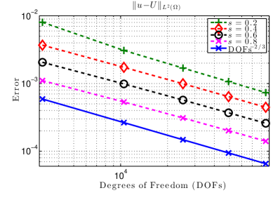
Figure 1: Rate of convergence on anisotropic meshes for $N=2$ and $s=0.2,0.4,0.6$ and $s=0.8$ is shown. $U$ is the numerical solution to (4.1) obtained by using Newton’s method. On the other hand, $u$ is the exact solution given by (4.5). The blue line is the reference line. The left panel shows the $\mathbb{H}^{s}(\Omega)$-error, in all cases we recover $(\#\mathscr{T}{Y})^{-1/3}$. The right panel shows the $L^{2}$-error which decays as $(\#\mathscr{T}{Y})^{-2/3}$.

References

- [1] N. Abatangelo and L. Dupaigne. Nonhomogeneous boundary conditions for the spectral fractional laplacian. Annales de l’Institut Henri Poincare (C) Non Linear Analysis, 2016, to appear.
- [2] S. Abe and S. Thurner. Anomalous diffusion in view of Einstein’s 1905 theory of Brownian motion. Physica A: Statistical Mechanics and its Applications, 356(2–4):403 – 407, 2005.
- [3] R.A. Adams. Sobolev Spaces. Academic Press [A subsidiary of Harcourt Brace Jovanovich, Publishers], New York-London, 1975. Pure and Applied Mathematics, Vol. 65.
- [4] T.M. Atanackovic, S. Pilipovic, B. Stankovic, and D. Zorica. Fractional Calculus with Applications in Mechanics: Vibrations and Diffusion Processes. John Wiley & Sons, 2014.
- [5] E. Barkai, R. Metzler, and J. Klafter. From continuous time random walks to the fractional Fokker-Planck equation. Phys. Rev. E (3), 61(1):132–138, 2000.
- [6] M. Biegert and M. Warma. Some quasi-linear elliptic equations with inhomogeneous generalized Robin boundary conditions on “bad” domains. Adv. Differential Equations, 15(9-10):893–924, 2010.
- [7] J.-P. Bouchaud and A. Georges. Anomalous diffusion in disordered media: statistical mechanisms, models and physical applications. Phys. Rep., 195(4-5):127–293, 1990.
- [8] C. Bucur and E. Valdinoci. Nonlocal diffusion and applications. arXiv:1504.08292, 2015.
- [9] A. Bueno-Orovio, D. Kay, V. Grau, B. Rodriguez, and K. Burrage. Fractional diffusion models of cardiac electrical propagation: role of structural heterogeneity in dispersion of repolarization. J. R. Soc. Interface, 11(97), 2014.
- [10] X. Cabré and J. Tan. Positive solutions of nonlinear problems involving the square root of the Laplacian. Adv. Math., 224(5):2052–2093, 2010.
- [11] L. Caffarelli and L. Silvestre. An extension problem related to the fractional Laplacian. Comm. Part. Diff. Eqs., 32(7-9):1245–1260, 2007.
- [12] L.A. Caffarelli and P.R. Stinga. Fractional elliptic equations, Caccioppoli estimates and regularity. Ann. Inst. H. Poincaré Anal. Non Linéaire, 33(3):767–807, 2016.
- [13] A. Capella, J. Dávila, L. Dupaigne, and Y. Sire. Regularity of radial extremal solutions for some non-local semilinear equations. Comm. Part. Diff. Eqs., 36(8):1353–1384, 2011.
- [14] L. Chen. Sobolev spaces and elliptic equations. 2011. http://www.math.uci.edu/~chenlong/226/Ch1Space.pdf.
- [15] W. Chen. A speculative study of -order fractional laplacian modeling of turbulence: Some thoughts and conjectures. Chaos, 16(2):1–11, 2006.
- [16] L. Debnath. Fractional integral and fractional differential equations in fluid mechanics. Fract. Calc. Appl. Anal., 6(2):119–155, 2003.
- [17] L. Debnath. Recent applications of fractional calculus to science and engineering. Int. J. Math. Math. Sci., (54):3413–3442, 2003.
- [18] D. del Castillo-Negrete, B. A. Carreras, and V. E. Lynch. Fractional diffusion in plasma turbulence. Physics of Plasmas, 11(8):3854–3864, 2004.
- [19] E. Di Nezza, G. Palatucci, and E. Valdinoci. Hitchhikerʼs guide to the fractional Sobolev spaces. Bulletin des Sciences Mathématiques, 136(5):521–573, 2012.
- [20] M. Doman. Weak uniform rotundity of Orlicz sequence spaces. Math. Nachr., 162:145–151, 1993.
- [21] P. Gatto and J. S. Hesthaven. Numerical approximation of the fractional laplacian via hp-finite elements, with an application to image denoising. J. Sci. Comp., 65(1):249–270, 2015.
- [22] V. Gol′dshtein and A. Ukhlov. Weighted Sobolev spaces and embedding theorems. Trans. Amer. Math. Soc., 361(7):3829–3850, 2009.
- [23] R. Gorenflo, F. Mainardi, D. Moretti, and P. Paradisi. Time fractional diffusion: a discrete random walk approach. Nonlinear Dynam., 29(1-4):129–143, 2002. Fractional order calculus and its applications.
- [24] G. Grubb. Regularity of spectral fractional dirichlet and neumann problems. Math. Nachr., 2015.
- [25] R. Ishizuka, S.-H. Chong, and F. Hirata. An integral equation theory for inhomogeneous molecular fluids: The reference interaction site model approach. J. Chem. Phys, 128(3), 2008.
- [26] D. Kinderlehrer and G. Stampacchia. An Introduction to Variational Inequalities and their Applications. Academic Press, New York, 1980.
- [27] A. Kufner and B. Opic. How to define reasonably weighted Sobolev spaces. Comment. Math. Univ. Carolin., 25(3):537–554, 1984.
- [28] S. Z. Levendorskiĭ. Pricing of the American put under Lévy processes. Int. J. Theor. Appl. Finance, 7(3):303–335, 2004.
- [29] J.-L. Lions and E. Magenes. Non-homogeneous boundary value problems and applications. Vol. I. Springer-Verlag, New York-Heidelberg, 1972. Translated from the French by P. Kenneth, Die Grundlehren der mathematischen Wissenschaften, Band 181.
- [30] R.R. Nigmatullin. The realization of the generalized transfer equation in a medium with fractal geometry. Physica Status Solidi (b), 133(1):425–430, 1986.
- [31] R.H. Nochetto, E. Otárola, and A. J. Salgado. A PDE approach to fractional diffusion in general domains: A priori error analysis. Found. Comput. Math., 15(3):733–791, 2015.
- [32] R.H. Nochetto, E. Otárola, and A.J. Salgado. A PDE approach to space-time fractional parabolic problems. arXiv:1404.0068, 2014.
- [33] A.I. Saichev and G.M. Zaslavsky. Fractional kinetic equations: solutions and applications. Chaos, 7(4):753–764, 1997.
- [34] P.R. Stinga and J.L. Torrea. Extension problem and Harnack’s inequality for some fractional operators. Comm. Part. Diff. Eqs., 35(11):2092–2122, 2010.
- [35] B.O. Turesson. Nonlinear potential theory and weighted Sobolev spaces, volume 1736 of Lecture Notes in Mathematics. Springer-Verlag, Berlin, 2000.
- [36] M. Warma. The fractional relative capacity and the fractional Laplacian with Neumann and Robin boundary conditions on open sets. Potential Anal., 42(2):499–547, 2015.