Scale Invariant Interest Points with Shearlets

Abstract

Shearlets are a relatively new directional multi-scale framework for signal analysis, which have been shown effective to enhance signal discontinuities such as edges and corners at multiple scales. In this work we address the problem of detecting and describing blob-like features in the shearlets framework. We derive a measure which is very effective for blob detection and closely related to the Laplacian of Gaussian. We demonstrate the measure satisfies the perfect scale invariance property in the continuous case. In the discrete setting, we derive algorithms for blob detection and keypoint description. Finally, we provide qualitative justifications of our findings as well as a quantitative evaluation on benchmark data. We also report an experimental evidence that our method is very suitable to deal with compressed and noisy images, thanks to the sparsity property of shearlets.

1 Introduction

Feature detection consists in the extraction of perceptually interesting low-level features over an image, in preparation of higher level processing tasks. In the last decade a considerable amount of work has been devoted to the design of effective and efficient local feature detectors able to associate with a given interesting point also scale and orientation information. Scale-space theory has been one of the main sources of inspiration for this line of research, providing an effective framework for detecting features at multiple scales and, to some extent, to devise scale invariant image descriptors.

In this work we refer in particular to blob features, image regions which are approximately uniform. In early works the Laplacian of the Gaussian (LoG) operator has been proposed as a way of enhancing blob-like structures [1]. Later, difference of Gaussians (DoG) has been introduced as an efficient approximation of the Laplacian [2], while the Hessian determinant [1] was suggested as an alternative operator with a higher sensitivity and better invariance properties. Later on, computationally efficient variants have also been devised [3, 4]. Since feature detection often precedes feature matching, local features need to be associated with an appropriate descriptor. For a reliable feature matching, it is important to identify a descriptor able to deal with geometric transformations, illumination changes, and the presence of noise. Therefore over the years there has been a lot of work in devising feature descriptors able to address different types of variations [5, 6, 2, 3, 7, 8]. It should be noticed how, in this context, much effort has been devoted to reducing the computational cost — it is worth mentioning the well known SIFT [2] and SURF [3] feature descriptors, obtained from scale-normalized derivatives in a scale-space representation based on image pyramids to speed up computation. More recently compact representations have been obtained by means of binary descriptors [9, 10, 11].

Unsurprisingly, image feature detection at multiple scales has also been addressed in the context of wavelet theory[12, 13, 14, 15, 16, 17, 18]. This framework allows for a natural derivation of the feature scale [12, 18] and for the design of perfect scale-invariant measurements [19]. It is equivalent to the scale-space representation it the mother wavelet is the derivative of the Gaussian [12], but it also allows for the choice of different mother functions to better enhance specific features.

While for 1D signals, wavelets and space-scale theory are the canonical multi-scale representations, for 2D signals there is a large class of representations with a further sensitivity to directional information, useful to deal with rotation invariance — here it is worth mentioning directional wavelets [20], contourlets [21], complex wavelets [22], ridgelets [23], curvelets [24], and shearlets [25].

In this paper we focus on shearlets representation and we show how local extremas of the shearlet coefficients may enhance blob structures in an image providing [26],

• a clear definition of these interest points;

• a well-defined position in image space;

• a local image structure with a rich directional information content;

• a stable procedure with an high degree of repeatibillity against noise and deformations;

• the capability to detect other interesting point, like edges and cornes, with a different choice of the generating function [27];

• an automatic scale selection with a scale invariant descriptor.

Indeed, shearlets enjoy different interesting properties which are meaninful to feature detection and description:

• As in the space-scale approach, the filters give rise to a coarse-to-fine multi-scale representation, but for shearlets two consecutive scales are related by an anisotropic dilation with ratio $1/\sqrt{2}$ and this anisotropy is the key property to have (optimal) sparse representation for natural images [28]. Among the multi-scale representations, only shearlets and curvelets ensure this kind of optimality, so that shearlets are appealing in applications dealing with signal compression.

• The shearlet coefficients directly encode directional information, unlike scale-space representations and traditional wavelets where one could derive directional information only as a post-processing, for example by computing the ratio between the partial derivatives.

• The rotational invariance of the representation is given by a shearing which preserves the rectangular lattice of the digital image, so that a faithful digital implementation is easy to obtain.

• In contrast to the scale-space approaches, with shearlets we have a large choice of admissible templates allowing to tune the shearlet transform to specific applications, e.g, the Gaussian derivative to locate edges or corners as in [29, 27], or the Mexican hat to analyze blob structures or ridge points.

• Shearlets also appear to have a potential in providing meaningful descriptions, although this capability has not been largely explored so far (see, for instance, [30, 31]).

In this paper, first, we provide an analysis of perfect scale invariance properties in the continuous case, similar to the study carried out by Lindberg for the scale-space [32]. Then, we derive a discretized formulation of the problem, obtaining a discrete measure which will be the main building block of our algorithms. This measure, obtained by summing up coefficients over all the shearing, is naturally isotropic, but we can easily recover the directional information by looking at the single coefficient.

Next, we propose an algorithm for detecting and describing blob-like features. The main peculiarity of our approach is in the fact it fully exploits the expressive power of the shearlet transform. Indeed, each detected feature is associated with a scale, an orientation, and a position, directly related with the dilation, the shearing and the translation provided by the underlying transformation. In the description phase we also use shearlets coefficients, orienting the contributions with respect to the estimated feature orientation. We underline how all the steps of our procedure are based on the same image transformation. In this sense the procedure is elegant and clean and has a potential in computational efficiency.

We present a comparative analysis on benchmark data where we show that the proposed method compares favorably with the state of the art of scale-space features. We also present a further experiment on a larger set of images, where we underline the appropriateness of the method to address image matching at different compression and noise levels. In this specific aspect resides one of the main contribution of our work from the application standpoint: the sparsity properties of the shearlet transform are very appropriate to deal with noise and compression artifacts.

The paper is organized as follows: In Section 2 we review the shearlet transform. Section 3 provide an analysis of scale selection in multi-scale image representations and the theoretical justifications of scale invariance for feature detection by shearlets. In Section 4 we propose the shearlet based blob detection algorithm, while the descriptor is introduced in Section 5. Section 6 reports a experimental analysis of the proposed blob detector and descriptor following the Oxford evaluation procedure. In Section 7 we evaluate the proposed methods for image matching at different compression and noise levels. Section 8 is left to a final discussion.

2 A Review of the Shearlet Transform

A shearlet is generated by the dilation, shearing and translation of a function $\psi\in L^{2}(\mathbb{R}^{2})$, called the mother shearlet, in the following way

$$\psi_{a,s,t}(x)=a^{-3/4}\psi(A^{-1}_{a}S^{-1}_{s}(x-t))$$ (1)

where $t\in\mathbb{R}^{2}$ is a translation, $A_{a}$ is a dilation matrix and $S_{s}$ a shearing matrix defined respectively by

$$A_{a}=\begin{pmatrix}a&0\\ 0&\sqrt{a}\end{pmatrix}\qquad S_{s}=\begin{pmatrix}1&s\\ 0&1\end{pmatrix},$$

with $a\in\mathbb{R}^{+}$ and $s\in\mathbb{R}$. The anisotropic dilation $A_{a}$ controls the scale of the shearlets, by applying a different dilation factor along the two axes. The shearing matrix $S_{s}$, not expansive, determines the orientation of the shearlets. The normalization factor $a^{-3/4}$ ensures that $\|\psi_{a,s,t}\|=\|\psi\|$, where $\|\psi\|$ is the norm in $L^{2}(\mathbb{R}^{2})$. The shearlet transform ${\mathcal{SH}}(f)$ of a signal $f\in L^{2}(\mathbb{R}^{2})$ is defined by

$${\mathcal{SH}}(f)(a,s,t)=\langle f,\psi_{a,s,t}\rangle$$ (2)

where $\langle f,\psi_{a,s,t}\rangle$ is the scalar product in $L^{2}(\mathbb{R}^{2})$.

In the classical setting the mother shearlet $\psi$ is assumed to factorize in the Fourier domain as

$$\hat{\psi}(\omega_{1},\omega_{2})=\hat{\psi}_{1}(\omega_{1})\hat{\psi}_{2}(\frac{\omega_{2}}{\omega_{1}})$$ (3)

where $\hat{\psi}$ is the Fourier transform of $\psi$, $\psi_{1}$ is a one dimensional wavelet and $\hat{\psi_{2}}$ is any non-zero square-integrable function.

With the choice of Eq. (3) the shearlet definition in the frequency domain (see Fig. 1) becomes

$$\hat{\psi}_{a,s,t}(\omega_{1},\omega_{2})=a^{3/4}\hat{\psi}_{1}(a\omega_{1})\hat{\psi}_{2}\left(\frac{\omega_{2}+s\omega_{1}}{\sqrt{a}\,\omega_{1}}\right)e^{-2\pi i(\omega_{1},\omega_{2})\cdot t}.$$

Figure 1: Support of the shearlets $\hat{\psi}_{a,s,t}$ (in the frequency domain) for different values of $a$ and $s$.

As a consequence of the Plancherel formula, Eq. (2) can be rewritten as

$${\mathcal{SH}}(f)(a,s,t_{1},t_{2})=a^{3/4}\int\limits_{\widehat{R}^{2}}\hat{f}(\omega_{1},\omega_{2})\hat{\psi}_{1}(a\omega_{1})\\ \times\hat{\psi}_{2}\left(\frac{\omega_{2}+s\omega_{1}}{\sqrt{a}\,\omega_{1}}\right)e^{2\pi i\xi\left(t_{1}\omega_{1}+t_{2}\omega_{2}\right)}d\omega_{1}d\omega_{2}.$$ (4)

A different approach is proposed in [33] where the mother shearlet is of the form $\psi_{1}(x_{1})\psi_{2}(x_{2})$, where $\psi_{1}$ is a one dimensional wavelet and $\psi_{2}$ is a scaling function. This property allows to have compact support shearlets in the space domain. However, as noted in [34], “ The property [of (3)] does indeed not only improve the frame bounds of the associated system, but also improves the directional selectivity significantly”. To overcome this problem, in [34] the mother shearlet is multiplied by a suitable 2D fan filter in order to approximate the property (3). For sake of simplicity, in this short review we consider only classical shearlets — the ones we have adopted in our work.

2.1 Cone-adapted Shearlets

A major limitation of the shearlets defined in the previous section is the directional bias of shearlet elements associated with large shearing parameters. To deal with this problem [28] introduces the notion of cone-adapted shearlets whose construction is based on a partition of the Fourier into two cones and a square centered around the origin. The two conic regions are defined as

$$\mathcal{C}_{\mathrm{h}} =\{(\omega_{1},\omega_{2})\in\mathbb{R}^{2}:|\omega_{2}/\omega_{1}|\leq 1,|\omega_{1}|>1\}$$

$$\mathcal{C}_{\mathrm{v}} =\{(\omega_{1},\omega_{2})\in\mathbb{R}^{2}:|\omega_{1}/\omega_{2}|\leq 1,|\omega_{2}|>1\}.$$

A shearlet $\psi$ suitable for the horizontal cone is

$$\hat{\psi}^{\mathrm{h}}(\omega_{1},\omega_{2})=\hat{\psi}_{1}(\omega_{1})\hat{\psi}_{2}\left(\frac{\omega_{2}}{\omega_{1}}\right)\chi_{\mathcal{C}_{\mathrm{h}}}(\omega_{1},\omega_{2}).$$

where $\chi_{\mathcal{C}_{\mathrm{h}}}(\omega)$ is equal to 1 for $\omega\in\mathcal{C}_{\mathrm{h}}$ and 0 outside. Likewise the shearlet for the vertical cone is defined by interchanging roles of $\omega_{1}$ and $\omega_{2}$.

The square region is the low-frequency part

$$\{(\omega_{1},\omega_{2})\in\mathbb{R}^{2}:|\omega_{1}|,|\omega_{2}|\leq 1\}.$$

Since the interest points of an image are associated with high frequencies, for space reason we do not consider the low-frequency contribution, see [28] for further details.

2.2 Digital Shearlets

Digital shearlet systems are defined by sampling continuous shearlet systems on a discrete subset of the space of parameters $\mathbb{R}_{+}\times\mathbb{R}^{3}$ and by sampling the signal on a grid. In the literature there are many different discretization schemes, see [35, 34] and reference therein. In this work we adopt the Fast Finite Shearlet Transform (FFST) [36] which performs the entire shearlet construction in the Fourier domain. It is possible to choose as $\Psi_{1}$ wavelets whose analytic form is given in the Fourier domain, whereas in [29] and [34] are restricted to wavelets associated with multiresolution analysis. In this scheme, the signal is discretized on a square grid of size $N$, which is independent of the dilation and shearing parameter, whereas the scaling, shear and translation parameters are discretized as

$$a_{j} =2^{-j},\quad j=0,\dots,j_{0}-1,$$

$$s_{j,i} =i2^{-j/2},\quad-\lfloor 2^{j/2}\rfloor\leq i\leq\lfloor 2^{j/2}\rfloor,$$

$$t_{m} =\left(\frac{m_{1}}{N},\frac{m_{2}}{N}\right),\quad m\in\mathcal{I}$$

where $j_{0}$ is the number of considered scales and $\mathcal{I}=\{(m_{1},m_{2}):m_{1},m_{2}=0,\dots,N-1\}$. With respect to the original implementation we use a dyadic scale $2^{-j}$ instead of $4^{-j}$ to reduce the difference among two consecutive scales, which is consistent with the discretization lattice in [34].

With these notations the shearlet system becomes

$$\psi^{\mathrm{x}}_{{j,i,m}}(x)=\psi^{\mathrm{x}}_{a_{j},s_{j,i},t_{m}}(x)$$

where $\mathrm{x}=\mathrm{h}$ or $\mathrm{x}=\mathrm{v}$ and the discrete shearlet transform of an digital image $\mathcal{I}$ is

$${\mathcal{SH}}(\mathcal{I})(j,\mathrm{x},i,m)=\langle\mathcal{I},\psi^{\mathrm{x}}_{j,i,m}\rangle$$

where $j=0,\dots,j_{0}-1$, $\mathrm{x}=\mathrm{h},\mathrm{v}$, $|i|\leq\lfloor 2^{j/2}\rfloor$, $m\in\mathcal{I}$. Based on the Plancherel formula $\langle f,g\rangle=\frac{1}{N^{2}}\langle\hat{f},\hat{g}\rangle$, the discrete shearlet transform can be computed by applying the 2D Fast Fourier Transform (fft) and its inverse (ifft). For example, for the horizontal cone ${\mathcal{SH}}(\mathcal{I})(j,\mathrm{h},i,m)$ is given by

$$2^{-\frac{3j}{4}}\texttt{ifft}(\hat{\psi}_{1}(2^{-j}\omega_{1})\hat{\psi_{2}}(2^{j/2}\frac{\omega_{2}}{\omega_{1}}+i)\texttt{fft}(\mathcal{I}))(m).$$ (5)

2.3 Shearing and Orientation

Figure 2: A visualization, in the Fourier domain for scale $j=2$, of the shearing indices $i$ on the horizontal and vertical cone (gray and white areas respectively), the complete ordering of index $k$, and the associated angles $\theta_{k}$.

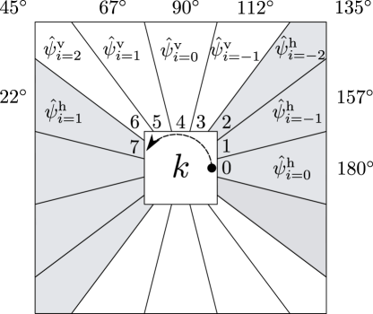
As we can notice, all the shearing associated with a scale $j$ are distributed along the two vertical and horizontal cones ${\mathrm{x}}$. For the sake of clarity, in order to provide a simple access to a specific shearing at a scale $j$, we introduce an index $k$ (similar to [36]) which replaces the shearing parameter $i$ and the cone parameters ${\mathrm{x}}=\{\mathrm{h},\mathrm{v}\}$ and simplifies the notation. For each scale $j$, the index $k$ iterates counter-clockwise the shearlets in the Fourier domain. It starts in the horizontal cone for each $i=-1,\ldots,-\lfloor 2^{j/2}\rfloor$ starting from $i=0$. Then, it continues iterating the vertical cone for $i=-\lfloor 2^{j/2}\rfloor+1,\ldots,\lfloor 2^{j/2}\rfloor$. Once the vertical cone is completed, it starts on the remaining of the horizontal cone, $i=\lfloor 2^{j/2}\rfloor-1,\ldots,1$. Figure 2 illustrates the relationship between the original index $i$ and $k$. Hence, from now on, we will consider the following formulation of the discrete shearlet transform

$${\mathcal{SH}}(\mathcal{I})(j,k,m)={\mathcal{SH}}(\mathcal{I})(j,\mathrm{x},i,m)\quad k=0,\ldots,4\lfloor 2^{j/2}\rfloor{-1},$$

where $4\lfloor 2^{j/2}\rfloor$ is the total number of shearlets for a scale $j$.

Now, we may associate an orientation $\theta_{k}$ to each index $k$:

$$\theta_{k}=\pi\left(1-\frac{k}{4\lfloor 2^{j/2}\rfloor}\right).$$ (6)

3 Scale Selection with Shearlets

Multi-scale frameworks, like scale-space, wavelets and shearlets, represent image structures at multiple scales and are thus appropriate for detecting structures or features with different spatial extent. They may also be effective in estimating an appropriate scale to a given detected feature, useful for further tasks such as matching or recognition. According to Lindeberg [37], the formal definition of scale selection refers to the estimation of characteristic scales in image data and the automatical selection locally appropriate scales in a scale-space representation.

A particularly useful methodology for computing estimates of characteristic scales is by detecting local extrema over scales of differential expressions in terms of $\gamma$-normalized derivatives [1]. Following this approach, it can be shown that different types of scale invariant feature detectors can be used for different types of visual features, like blobs, corners, etc. Furthermore, the scale levels obtained from the scale selection can be used for computing image descriptors.

Detected feature points are considered scale invariant if the points are preserved under scaling transformations and the selected scale levels are transformed in accordance with the amount of scaling [1]. In addition, perfect scale invariance is considered when the extrema over scales are equal.

In this section, we start from the continuous setting and first discuss scale invariance properties reviewing Lindeberg approach in the framework of space-scale theory [1]. Then, we show how shearlet coefficients can also detect the correct scale while providing directional information. In the second part of the section we discuss how we can obtain a measure of scale in the discrete setting.

3.1 Scale Invariance in the Continuous Setting

When a signal is subject to a scale-space smoothing, the spatial derivatives on the smoothed data are expected to decrease. This is a well-known property of the scale-space representation, according to which the amplitude of its spatial derivatives decreases with scale. To obtain a multi-scale signal representation whose amplitude is independent on the scale Lindeberg proposed a $\gamma$-normalized derivative operator [1]. In this section, we will show that shearlets share a similar behaviour, but they directly encode the directional information. We observe how a similar analysis could be carried out considering directional wavelets [20], which are not included in our study but will be taken into account in future works.

3.1.1 Scale-space

In this section we briefly recall the main properties of scale-space theory for two dimensional signals developed by Lindeberg [1].

In the scale-space theory, the filters are given by the family of 2D-Gaussian kernels

$$g_{a}(x)=\frac{1}{2\pi a^{2}}e^{-\frac{x^{2}}{2a^{2}}}\qquad x\in\mathbb{R}^{2}$$

parametrised by the scale $a\in\mathbb{R}^{+}$. Each signal $f$ is mapped to its scale-space transform by convolution with $g_{a}$

$$L[f](a,z) =g_{a}\ast f(az)=\int_{\mathbb{R}^{2}}g_{a}(y)f(az-y)dy$$

where $z=x/a$ is the “scale invariant” space variable. In the original paper [1] the scale is $t=a^{2}$ and a more general rescaling is considered ( as for example $z=x/t^{\gamma/2}$). This representation has two main properties, which are at the root of the theory and are usually referred as perfect scale invariance. First, the representation $L[f]$ is invariant under dilations, i.e. if $f_{\alpha}(x)=f(x/\alpha)$ with $\alpha\in\mathbb{R}^{+}$, then

$$L[f_{\alpha}](a,z)=L[f](\alpha^{-1}a,z).$$

Furthermore, for 2D sinusoidal signals

$$f(x_{1},x_{2})=\cos(\alpha x_{1})\cos(\beta x_{2}),$$ (7)

the corresponding transform is able to detect the scale by applying a suitable differential operator

$$\mathcal{D}=P(\frac{\partial}{\partial z_{1}},\frac{\partial}{\partial z_{2}})$$

where $P$ is a given polynomial in two variables. Indeed, define the quantity

$$L_{\mathcal{D},\max}(a)=\max_{z\in\mathbb{R}^{2}}|\mathcal{D}L[f](z,a)|,$$

since

$$L[f](a,z)=e^{-\frac{a^{2}(\alpha^{2}+\beta^{2})}{2}}f(az),$$

then

$$L_{\mathcal{D},\max}(a)=P(a\alpha,a\beta)e^{-\frac{a^{2}}{2}(\alpha^{2}+\beta^{2})}.$$ (8)

For example, if $\mathcal{D}=\frac{\partial^{2}}{\partial z_{1}^{2}}+\frac{\partial^{2}}{\partial z_{2}^{2}}$ is the $z$-Laplacian, then

$$L_{\mathcal{D},\max}(a)=a^{2}(\alpha^{2}+\beta^{2})e^{-\frac{a^{2}}{2}(\alpha^{2}+\beta^{2})},$$

which takes its maximum at ${a^{*}=1/\sqrt{\alpha^{2}+\beta^{2}}}$ with value independent on the scale. Hence, the extrema of the scale-space representation across the scale $a$ allows to detect the scale $1/\sqrt{\alpha^{2}+\beta^{2}}$ of the signal. However, to extract the ratio $\beta/\alpha$ associated with the directional information there is the need to compute other quantities as the determinant of the Hessian [26]. In the next section we show that shearlets have essentially the same behaviour, but the transform directly detect both the parameters $\alpha$ and $\beta$.

3.1.2 Shearlets

Since the dilation matrix defining the shearlets is not isotropic, we can not expect that the shearlet transform itself is invariant under (isotropic) scale changes. However, we will show how a related quantity has the perfect scale invariance property, as demonstrated by the following result, whose proof can be found in the appendix.

Theorem.

The rotationally invariant shearlet transform

$$B[f](a,z)=a^{-5/4}\int_{\mathbb{R}}\mathcal{SH}(f)(a,s,az)ds,$$ (9)

with $a\in\mathbb{R}_{+}$ and $z\in\mathbb{R}^{2}$, is scale invariant, i.e. for all $f\in L^{2}(\mathbb{R}^{2})$

$$B[f_{\alpha}](a,z)=B[f](\alpha^{-1}a,z).$$

Furthermore, if $f$ is the sinusoidal signal given by (7), then

$$B[f](a,z)=\overline{\psi_{2}(0)}\overline{\hat{\psi_{1}}(\frac{a\alpha}{2\pi})}f(az),$$

provided that $\Psi_{1}$ is even.

As we did for scale-space, if $f$ is the 2D sinusoidal signal as in (7) a simple calculation shows that the maximum of the modulus over $z$ is

$$B_{\max}[f](a)=|\psi_{2}(0)|\,|\hat{\psi_{1}}(\frac{a\alpha}{2\pi})|.$$ (10)

By choosing $\hat{\psi}_{1}$ as the $1D$-Mexican hat wavelet

$$\hat{\psi_{1}}(\omega)=\omega^{2}e^{-2\pi^{2}\omega^{2}},$$ (11)

we can rewrite Eq. (10) as

$$B_{\max}[f](a)=\frac{|\psi_{2}(0)|}{4\pi^{2}}(a\alpha)^{2}e^{-\frac{(a\alpha)^{2}}{2}},$$ (12)

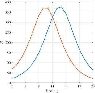
which shares the same behaviour of $L_{\max}[f]$, but the maximum of $B_{\max}[f]$ is now at $a^{*}=1/\alpha$. Hence, for shearlets the selected scale $a^{*}$ only depends on the frequency $\alpha$, as shown in Fig. 3. However, if we consider the shearlet coefficient, a computation as above shows that

$$\max_{t\in\mathbb{R}^{2}}|\mathcal{SH}(f)(a,s,t)|=a^{3/4}|\hat{\psi_{1}}(\frac{a\alpha}{2\pi})||\hat{\psi}_{2}(\frac{s+\beta\alpha^{-1}}{\sqrt{a}})|,$$

provided that both $\psi_{1}$ and $\psi_{2}$ are even. Since $\hat{\psi}_{2}$ is a bump function, fixed the scale $a$, the shearlet coefficients have a maximun around an interval centered at $s=-\beta/\alpha$. If $\hat{\psi}_{2}$ is a Gaussian bump and $\Psi_{1}$ is as in (11)

$$a^{-3/4}\max_{t\in\mathbb{R}^{2}}|\mathcal{SH}(f)(a,s,t)|=C(a\alpha)^{2}e^{-\frac{(a\alpha)^{2}}{2}}e^{-\frac{(s+\beta\alpha^{-1})^{2}}{2a}}.$$

(a) Scale-space

(b) Shearlets

Figure 3: The plot of (a) $L_{\max}(t)$ Eq. (8) and (b) $B_{\max}[f](a)$ Eq. (12) as function of scale for 2D sinusoidal signals at different frequencies $\alpha$ and $\beta$.

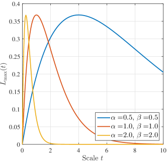
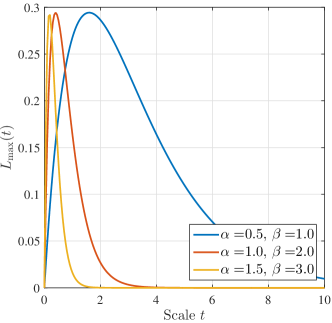
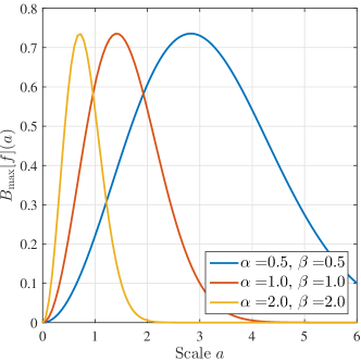
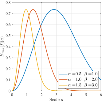
Fig. 3 presents the actual plots of Eq. (8) for the scale-space and Eq. (12) for shearlets at different combinations of the frequencies parameters $\alpha$ and $\beta$. In the plots on the left, the frequencies $\alpha$ and $\beta$ are equally increased by a factor of 2 (isotropic structures), while on the right, $\alpha$ is increased by a step equal to 0.5 and $\beta=2\alpha$ (anisotropic structures). As we can observe, the plots associated with both approaches are capable to produce perfect scale invariance for the two types of frequency combinations in the sinusoidal function $f$.

(a) 2D Gaussian functions with different $\sigma_{x},\sigma_{y}$

(b) Laplacian

(c) Shearlets

Figure 4: Scale decomposition of the synthetic images in (a) at their center point (color-coded) by using the (b) Laplacian of Gaussian, and (d) shearlet $\mathcal{B}$ measure.

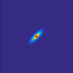
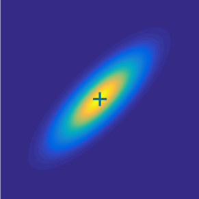
Finally, we stress that the choice of $\psi_{1}$ and $\psi_{2}$ influences the type of local features that are enhanced by the shearlet transform. Thus, in order to detect blob features, as suggested by Equation (11) we selected $\psi_{1}$ as the Mexican hat wavelet and $\psi_{2}$ as a smooth function with compact support whose analytic form is given in [36].

3.2 Scale Invariance in the Discrete Setting

In the previous section, we defined a scale invariant shearlet transform in the continuous setting. Now, let us formally define the discrete counterpart of Eq. (9), which we call the $\mathcal{B}$ measure.

Definition.

The $\mathcal{B}$ measure is the scale-normalized sum of the discrete shearlet transform coefficients across the shearing parameter,

$$\mathcal{B}(m,j)=\frac{2^{\frac{5j}{4}}}{C_{j}}\sum_{k}\mathcal{SH}(\mathcal{I})(j,k,m),$$ (13)

where $j,k,m$ are the discretized scaling, shearing and translation parameters.

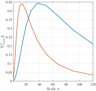
Comparing with Eq. (9), the normalization factor $C_{j}$ takes into account that for each scale $j$ there is a different number of orientations. We now briefly discuss the concept of perfect scale invariance on a discrete synthetic signal. Fig. 4 (a) shows two 2D Gaussian functions with different $\sigma_{x},\sigma_{y}$ and with an orientation of $\pi/4$. The $\sigma_{y}$ has a step of $1/3$ while the $\sigma_{x}=\sigma_{y}/3$, thus producing an elliptical structure at differen scales. In the rest of Fig. 4, we calculated the scales at the center point of each image with the following configurations. For scale-space, we used the scale-normalized Laplacian. For shearlets we used the $\mathcal{B}$ measure (Eq. (13)) and the 2-nd derivative of the Gaussian was used as $\psi_{1}$. By analyzing Fig. 4, we can observe that, by performing direct calculations, perfect scale-invariance still holds for the three discussed frameworks on syntectic images.

Figure 5: Space localization of blob features using the $\mathcal{B}$ measures at $j=0$.

4 Blob Detection with Shearlets

In this section we deal with the problem of automatically detecting blobs and describe our Shearlet Blob Detector (SBD) algorithm.

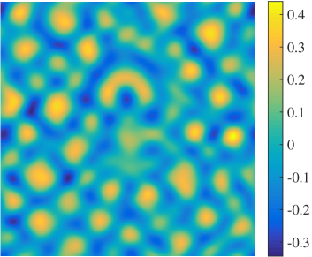
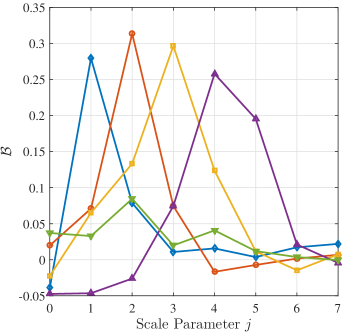
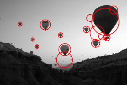
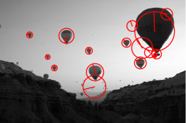
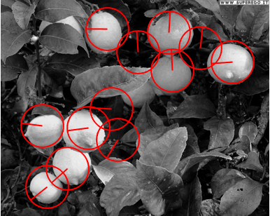
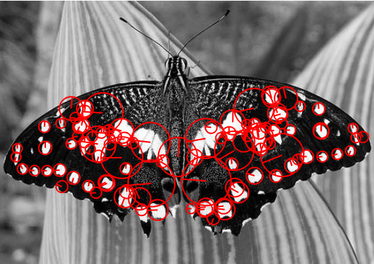
Let us first analyze separately the behavior of $\mathcal{B}$ in scale and space. Fig. 5 provides the result of the measure ${\cal B}$ computed at scale $j=0$. As we can observe, the biggest sunflower structures are correctly localized by obtaining a high value of $\mathcal{B}$ at the coarsest scale. Fig. 6 illustrates instead the behavior of ${\cal B}$ across scales for different key points of a real image. We consider in particular five locations corresponding to blob structures of different size and one texturized region. It is easy to observe that although there is no perfect scale invariance, the peaks are clearly visible and their position reflect the different spatial extents of the corresponding image structures.

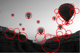
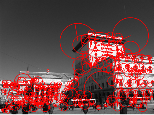
Similarly to the method proposed by Lowe to extract DoG features [2], our approach consists of different steps of measures, computation and refinement. In the reminder of the section we detail the three steps of the blob detection algorithm. Fig. 7 shows the intermediate steps results on a sample image.

  

Figure 6: The behavior of ${\cal B}$ across scales for different points, coherently color-coded.

4.1 Accurate feature point localization

A location $m$ at a certain scale $j$ is recognized as a candidate keypoint if the function $\mathcal{B}(m,j)$, computed over a spatial $3\times 3\times 3$ (2D space $\times$ scales) neighborhood centered on $m$ assumes a local extrema (maxima or minima) in it and its value is above a threshold.

$$(\bar{m},\bar{j})=\arg\underset{m,j}{\operatorname{\mathrm{maxmin}}}\ \mathrm{local}\ \mathcal{B}(m,j).$$ (14)

Then, the local extrema of the $\mathcal{B}$ function are interpolated in space and scale with the Brown and Lowe method [38] to reduce the effect of considering a limited number of scales. The outcome of this step is a set of feature points with their associated scales.

Notice that since the $\mathcal{B}$ measure is isotropic, only rotationally invariant features will be detected.

Figure 7: The different steps of the shearlet blob detector algorithm. Left: feature point localization; Centre: edge response elimination; Right: orientation assignment

Figure 8: Qualitative results of our blob detector on different scenarios.

4.2 Edge responses elimination

The function $\mathcal{B}$ has strong responses along edges, especially at fine scales. Therefore, in order to increase stability of the detected points, we need to eliminate the feature points that have high edge responses. By using the shearlet transform, we define $\varepsilon_{j}(m)$ as a metric that measures for a point $m$ at scale $j$ how spread out are the orientation responses with respect to the predominant orientation response. Formally,

$$\varepsilon_{j}(m)=\frac{1}{4\lfloor 2^{j/2}\rfloor}\left|\sum_{k}\left(\mathcal{SH}(\mathcal{I})(j,k,m)-\mathcal{SH}(\mathcal{I})(j,k_{\mathrm{max}},m)\right)^{2}\right|$$

where ${4\lfloor 2^{j/2}\rfloor}$ is the total number of shearings for scale $j$, and $k_{\max}$ is the shearing with larger shearlet response,

$$k_{\mathrm{max}}=\arg\max_{k}|{\mathcal{SH}}(\mathcal{I})(j,k,m)|.$$ (15)

High values of $\varepsilon_{j}(m)$ correspond to situations where $k_{\mathrm{max}}$ is the only orientation with strong support, that is, $m$ is an edge or close to an edge point. Conversely, the value of $\varepsilon_{j}(m)$ starts decreasing when the point $m$ has more than one, or none, predominant orientations. The second case corresponds to blob points.

Therefore, points $m$ with a high edge response may be deleted by an appropriate thresholding.

4.3 Accurate orientation assignment

In this step an orientation is assigned to each feature point. This is an important step with a view to the computation of rotation invariant local feature descriptors. By means of the shearlet transform, the predominant orientation at a point $m$ and scale $j$ is easily obtained by finding the index $k_{\mathrm{max}}$ given by Equation  (15). However, the orientation estimation at coarse scales may have low accuracy since for $j$ small a few shearings are employed. The effects can be attenuated by finding the extremum of an interpolated parabola for the following three points:

$$[\theta_{k_{\mathrm{max}}-1},{\mathcal{SH}}(\mathcal{I})(j,k_{\mathrm{max}}-1,m)]$$

$$[\theta_{k_{\mathrm{max}}},{\mathcal{SH}}(\mathcal{I})(j,k_{\mathrm{max}},m)]$$

$$[\theta_{k_{\mathrm{max}}+1},{\mathcal{SH}}(\mathcal{I})(j,k_{\mathrm{max}}+1,m)],$$

where $\theta_{k}$ is the angle associated with the shearing $k$, as in Eq. (6).

Fig. 8 reports outputs examples of our blob detector on a variety of scenarios. For all images, blobs have been detected using a shearlet transform with 8 scales, and a rather permissive threshold for edge points elimination. The circles indicating the presence of blobs have a radius proportional to the estimated optimal scale. As observed, such estimates are very close to the effective spatial extent of image structures.

5 Feature Description with Shearlets

In this section we propose a local feature descriptor based on the shearlet transform, the Shearlet Local Description algorithm (SLD).

The idea behind our descriptor is to encode the shearlet coefficients computed from the SBD, and thus complete the full detection-description pipeline with a single main computation, the shearlet transform in this case.

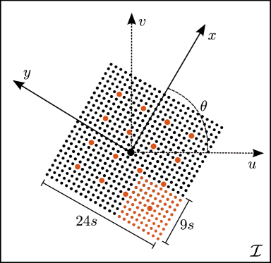
Given a feature $F=(m_{1},m_{2},j,\theta)$, where $m=(m_{1},m_{2})$ is its location, $j$ its estimated scale and $\theta$ its predominant orientation, our descriptor encodes the shearlet coefficients information from a square region centered on $(m_{1},m_{2})$, scaled with respect to $j$ and rotated according to $\theta$ (Fig. 10).

5.1 Shearings with common orientations

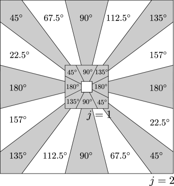
Since in our representation different scales are associated with different amount of shearings, we first need to fix a common number of shearings across scales, in order to obtain descriptions of equal size from keypoints at different scales. Moving towards finer scales, there is an inclusion relation between the corresponding range of shearings, thus the orientations associated to the shearings at coarser scales are also available at fine scales, see Fig. 9.

Let $O$ be a set of orientations that can be associated with the shearings of all the employed scales. The cardinality of the set is $|O|=c$, where $c$ is the only parameter of this method and will influence the size of the descriptor. By default, $O=\{180^{\circ},135^{\circ},90^{\circ},45\}$ since these are the orientations associated with the four shearlets of the coarser scales $j=0,1$.

We refer to $S_{j}$ as the sequence of all $4\lfloor 2^{j/2}\rfloor$ shearings for scale $j$, and to $S^{O}_{j}$ as the sequence of shearings in scale $j$ with respect to the common orientations $O$. Fig. 9 shows an example. For scale $j=2$, $S_{2}$ is composed by all the shearlets (white and grey), while $S^{O}_{2}$ is only composed by the gray shearlets. Notice that for $j=1$, $S^{O}_{1}$ is equal to $S_{1}$.

Figure 9: Visualization of the orientations at scales $j=1,2$ and $O=\{180^{\circ},135^{\circ},90^{\circ},45\}$. In gray: sequence of common orientations $S^{O}_{j}$. In white: orientations $S_{j}$. (see text).

5.2 Spatial sampling

We sample a regular grid of 24 points per side around $(m_{1},m_{2})$ with a sampling step of $s=2^{j_{0}-j}$, i.e. the inverse shearlet continuous scale of the feature, covering a length of $24s$.

We divide the regular grid in $16$ overlapped subregions of size $9s\times 9s$ (hence including 81 shearlet coefficients). We refer to each subregion using the centroid (thick red points in Fig. 10 (b)), which may be described by its relative position with respect to the local keypoint reference system. More formally, the subregions can be referred to as $\{\mathcal{G}_{e,f}\}$ where $e,f\in\{\pm 1,\pm 2\}$. Notice that the overlap allows us to cope with small spatial keypoint shifts.

Figure 10: Illustration of the change of coordinates for rotation invariance and the scaled and orientated shearlet sampled points used for the construction of the SLD descriptor.

5.3 Region rotation

In order to gain rotation invariance, we compute the actual descriptor on a region which is rotated according to the keypoint main orientation $\theta$. To this purpose, we perform a change of reference system (see Fig. 10),

$$\begin{pmatrix}x\\ y\end{pmatrix}=s\cdot\begin{pmatrix}\cos\theta&-\sin\theta\\ \sin\theta&\cos\theta\end{pmatrix}\begin{pmatrix}u\\ v\end{pmatrix}+\begin{pmatrix}m_{1}\\ m_{2}\end{pmatrix}.$$

To maintain the rotation invariance, the shearing parameter $k$ also has to be aligned according to $\theta$. To this purpose, we perform a circular shift following the shearing indexing $i_{k}$ described on Section 2.3,

$$t(k)=(i_{k}\pm n_{\theta})\ \mathrm{mod}\ |S_{j}|$$

where $n_{\theta}=\lfloor\theta|S_{j}|/\pi\rceil$ is the number if shifts required to align with respect to $\theta$.

5.3.1 Descriptor construction

The SLD descriptor concatenates statistics on shearlets coefficients in each subregion. We start by describing a subregion $\mathcal{G}_{e,f}$ of scale $j$ and shearing $k$ by a 2-D vector $\mu(e,f,j,k)$

$$\mu(e,f,j,k)=\begin{pmatrix}\sum_{(u,v)\in\mathcal{G}_{e,f}}M_{j}(u,v,k)g(u,v,2.5s),\\ \sum_{(u,v)\in\mathcal{G}_{e,f}}\left|M_{j}(u,v,k)\right|g(u,v,2.5s)\end{pmatrix}.$$

where

$$M_{j}(u,v,k)=\mathcal{SH}(\mathcal{I})(j,t(k),(x,y))$$

and $g$ is a 2D Gaussian filter with $\sigma=2.5s$. Then, within the subregion, we concatenate $\mu(e,f,j,k)$ for each shearing $k\in S^{O}_{j}$ following the order induced by the circular shift: let us denote it as $\mu(e,f,j)\in\mathbb{R}^{2\times c}$.

Remark: The rotation invariance can be improved by performing a weighted sum over the shearing neighbourhoods of the sampled point, instead of sampling directly into the shearlet coefficient. That is,

$$M_{j}(u,v,k)=\sum_{r=-|S_{j}/2|}^{|S_{j}/2|}\mathcal{SH}(\mathcal{I})(j,t(k+r),(x,y))g(r,\sigma)$$

where $g$ in this case is a 1D Gaussian with $\sigma=|S_{j}|/5$. This way small misalignments in the orientation can be overcome. However, the drawback is the additional computation.

Next, the contribution of each subregion is weighted using a Gaussian with $\sigma=1.5$. and then concatenated to build the descriptor $\mu\in\mathbb{R}^{2\times c\times 16}$ as

$$\mu=\left[\mu(e,f,j)g(e,f,1.5)\right]_{e,f\in\{\pm 1,\pm 2\}}.$$

Both Gaussian weighting increase robustness towards geometric deformations and localization errors [3].

5.3.2 Descriptor normalization

Finally, in order to gain invariance to linear contrast changes, we normalized the descriptor to a unit vector, using the $\ell_{2}$ normalization,

$$SLD(F)=\mu/\|\mu\|_{2}.$$ (16)

6 Experimental Results

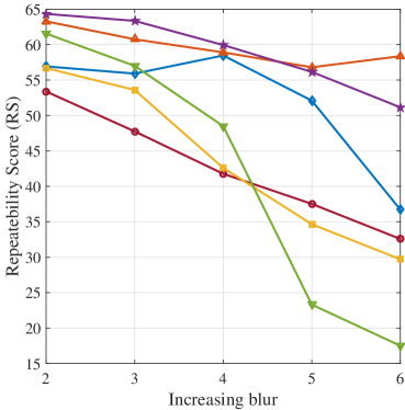
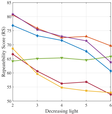
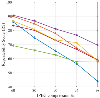
In this section we provide an experimental assessment of our shearlet-based method for blob detection and description. Our evaluation follows the Mikolajczyk’s protocol and image sequences implemented on VLBechmarks [39]. Each sequence includes 6 images of natural textured scenes with increasing geometric and photometric transformations.

(a) Graffiti

(b) Wall

(c) Boat

(d) Bark

(e) Bikes

(f) Trees

Figure 11: Comparison of multi-scale feature detection using repeatability scores ($40\%$ overlap error) with respect to viewpoint change (11a and 11b), scale change (11c and 11d) and image blur (11e and 11f).

(g) Leuven

(h) Ubc

Figure 11: Comparison of multi-scale feature detection using repeatability scores ($40\%$ overlap error) with respect to light change (11g) and image compression (11h).

6.1 Detection Evaluation

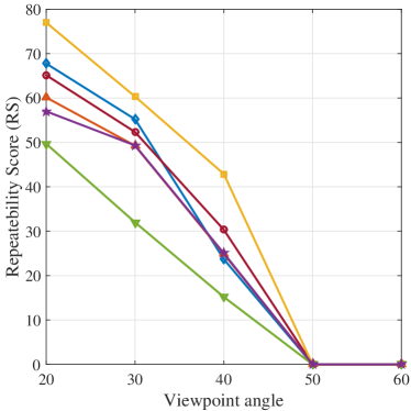
We evaluate the detection performances using the repeatability score (RS) [40], i.e. the ratio of the number of correspondences and the number of detected features. We compare the proposed Shearlet Blob Detector (SBD) with SIFT [2], Harris-Laplace [41], Hessian-Laplace [41], SURF [3] and BRISK [10] feature detectors. As for SIFT, Harris-Laplace and Hessian-Laplace we relied on the implementations provided with the VLBechmarks, while for SURF and BRISK, we adopted the implementation available in MATLAB. For a fair comparison, we adjust the thresholds of the detectors so that the number of detected keypoints is similar in the first image of the sequences.

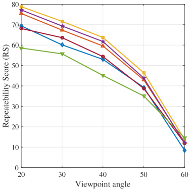
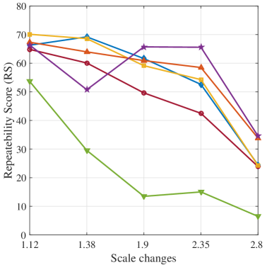
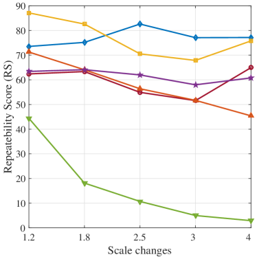
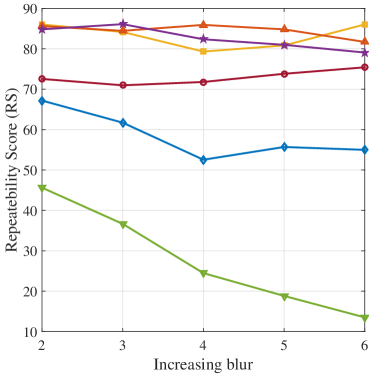
Figure 11 summarizes the obtained results and shows how our detector is appropriate under general circumstances, while there is no method which is clearly and uniformly superior to the others.

Viewpoint changes (Fig. 11a and 11b). On the Graffiti sequence, Hessian-Laplace outperforms the other methods that show comparative results with exception of BRISK. Hessian-Laplace, SBD and SURF outperforms the others detectors in that order on the Wall sequence.

Scale changes (Fig. 11c and 11d). On the Boat sequence, our method allows for higher repeatability as the scale change increases. SIFT and Hessian-Laplace are the best-performing methods on the Bark sequence.

Image blur (Fig. 11e and 11f). On the Bikes sequence, SURF, SBD and Hessian-Laplace outperform the other detectors with comparable results, while on the Tree sequence SBD outperforms the others detectors with the exception of the last transformation in which SURF obtains better repeatability.

Illumination changes (Fig. 11g). On the Leuven sequence, SBD and SURF outperform the rest of detectors. On the first half of the sequence they show very similar repeatability, while for the rest of the transformation SBD is outperformed by SURF.

JPEG compression (Fig. 11h). Overall, SBD outperforms the competitors, showing the ability to deal with increasing levels of signal compression.

6.2 Descriptor Evaluation

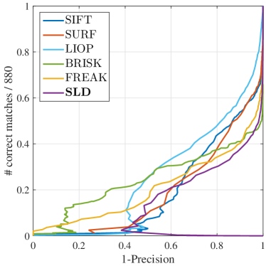
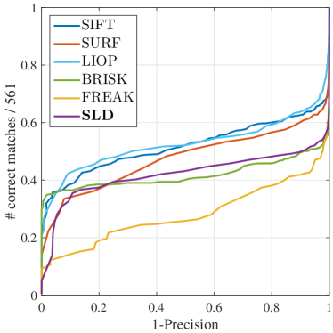
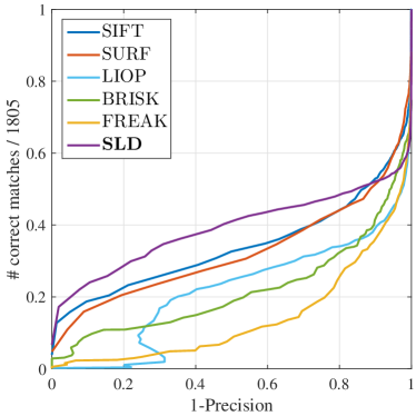
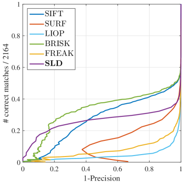
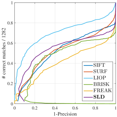
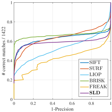
The Shearlet Local Descriptor (SLD) is evaluated using recall (number of correct matches / number of correspondences) vs 1-precision (number of false matches / number of matches) curves obtained by matching pairs of images ($1^{st}$ and $4^{th}$) from each sequence (as in [5]). As a comparative evaluation, we also report the results obtained using SIFT, SURF and LIOP [8] descriptors, along with the recent BRISK and FREAK [11] (implementation available in MATLAB). For all the descriptors we employed their default parameters included our SLD, for which we set $c=4$. Our default choice represents a compromise between computational efficiency and quality of the results. As for matching strategy, we used a threshold-based approach – where two detected blobs are matched if the distance between their descriptors is below a threshold – which is known to be indicative of the distribution of the descriptors in the space [5]. We employed the Euclidean distance for SLD, SIFT, SURF and LIOP, while we compare BRISK and FREAK (binary descriptors) using the Hamming distance. In order to maintain an unbiased comparison, we evaluate all the descriptors in combination with the DoG feature detector (the one usually coupled with SIFT) using the default parameters for all the image sequences. We now discuss the obtained results, reported in Figure 12.

Viewpoint changes (Fig. 12a). On the Graffiti sequence, BRISK and LIOP results as the best performing descriptor.

Scale changes (Fig. 12b). On the Boat sequence, SIFT and LIOP descriptors guarantee the highest accuracies, while our method provides intermediate performances.

Image blur (Fig. 12c and 12d). On the Bikes sequence, SLD outperforms the competitors, while SIFT and SURF show consistent results. BRISK is the best performing approach for the Trees sequence, while SLD provides a trade-off between SIFT and SURF results.

Illumination changes (Fig. 12e). On the Leuven sequence, LIOP is the best performing descriptor, while SLD outperforms the rest of the methods, except for very low precision values.

JPEG compression (Fig. 12f). On the UBC sequence, SLD, SIFT, SURF and BRISK show overall comparable results, while FREAK and LIOP provides poor performances.

In summary, here again, we do not observe a clear superiority of a method over the others. It should be noticed how our SLD behaves consistently well in the presence of blur, compression effects, illumination changes. This is explicable in terms of the properties of shearlets which provide us with an optimal sparse representation for natural images. The potential of shearlets under these circumstances is further evaluated in the next section.

(a) Graffiti

(b) Boat

(c) Bikes

(d) Trees

(e) Leuven

(f) UBC

Figure 12: Comparison of feature descriptors using Precision-Recall curves with respect to viewpoint change (12a), scale change(12b), image blur (12c and 12d), light change (12e), and image compression (12f).

(a) JPEG compression

(b) Gaussian noise corruption

Figure 13: Comparison of blob detectors with their respective descriptor on the INRIA Copydays dataset. Left: matching score against amount of compression (a) and noise corruption (b). Right: recall vs 1-precision curve between untransformed and 15 QF compressed (a) and 13 dB of SNR noise corrupted images.

7 Experiments on compressed and noisy images

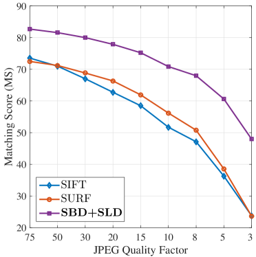
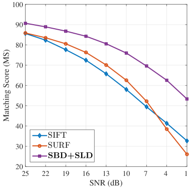
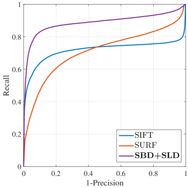
In this section we discuss the use of our full pipeline (SBD+SLD) on a larger set of images, and consider the problem of matching images characterised by different levels of compression and noise. We evaluate our results on the INRIA Copydays dataset, which contains 157 natural images that are progressively compressed, from 3 (very low quality) to 75 (typical web quality) quality factor (QF). For the evaluation in noisy environments, the images were also progressively corrupted with Gaussian noise.

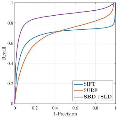
Our method is compared with the SIFT and SURF methods (DoG+SIFT and fastHessian+SURF, respectively). For the evaluation, we considered the Matching Score (MS) [40] which is the ratio between the number of correct matches and the number of detected features. For a visual impression of the overall performances, average values are reported. Fig. 13 (left) shows the comparison, where the matching superiority of our approach can be appreciated in both JPEG compression (a) and noise corruption (b).

As a further evidence, we also provide the recall vs 1-precision curve (see Fig. 13, right) obtained when matching the (untransformed) images with the compressed instances (15 quality factor) in (a) and noisy instances (13 dB of Signal to Noise Ratio) in (b). Note that our approach consistently outperforms the competitors.

The results we obtained are in good agreement with the theoretical intuition that shearlets are an appropriate choice in particular when dealing with noisy and compressed signals.

8 Conclusions

In this paper we considered the shearlet representation as a multi-scale framework for the detection and the description of scale-invariant interest points. We first provided a comparative analysis of scale invariance in the scale-space and shearlets domains, in the continuous case — following the reasoning proposed by Lindeberg [26]. Then, we considered a discrete setting and we addressed the problem of detecting and describing blob-like features by means of the shearlet transform, exploiting it capability of embedding naturally both scale and orientation information. More specifically, we proposed a Shearlet Blob Detector (SBD) algorithm and a Shearlet Local Descriptor (SLD) algorithm, which we experimentally assessed by a thorough evaluation on a benchmark dataset. Our algorithm compared favorably with the state of the art, showing a very good tolerance to blur, illumination variations and compression in particular. We also considered a larger dataset of images affected by different degrees of noise or compression degradation, showing how our shearlet-based pipeline, which includes both detection and description, provided superior results to SIFT and SURF.

In future works different shearlet transform alternatives will be worth investigating. In particular, compactly supported shearlets in the space domain [33] have been recently shown to have nice properties for edge detection [42] since they could allow us to capture effectively the spatial locality of image features. Since our proposed methods follows exactly the theoretical conceptual path of shearlets, another future work will be to provide a more efficient implementation of our methods based on approximation strategies and optimizations as in [2, 3]. Moreover, the process of computing the shearlet transform has an intrinsically parallel nature, thus a GPU implementation can provide a dramatic improvement, as shown in [43] for image denoising. By using the 3D shearlet transform [44], we also have the interest of extending the proposed shearlet detectors to 3D signals and video image sequences (2D + time).

Appendix A Proof of Theorem Theorem

Proof.

Let $\mathcal{SH}(f)(a,s,t_{1},t_{2})$ be the continuous shearlet transform of $f$ given by (4). With the change of variables $\omega_{1}=\xi$ and $\omega_{2}=v\xi$ whose Jacobian is

$$\left|\frac{\partial(\omega_{1},\omega_{2})}{\partial(\xi,v)}\right|=\left|\operatorname{det}\left[\begin{array}[]{cc}1&0\\ v&\xi\end{array}\right]\right|=|\xi|$$

Eq. (4) can be rewritten as

$$\mathcal{SH}(f)(a,s,t_{1},t_{2})=a^{3/4}\\ \times\int_{\mathbb{R}}\left\{\overline{\hat{\psi_{2}}\left(\frac{v-s}{\sqrt{a}}\right)}\left[\int_{\hat{\mathbb{R}}}\hat{f}(\xi,v\xi)\overline{\hat{\psi}_{1}(a\xi)}e^{2\pi i\xi\left(t_{1}+vt_{2}\right)}|\xi|d\xi\right]\right\}dv$$

where the inner integral

$$I(a,s,t_{1},t_{2},v)=\int_{\hat{\mathbb{R}}}\hat{f}(\xi,v\xi)\overline{\hat{\psi}_{1}(a\xi)}e^{2\pi i\xi\left(t_{1}+vt_{2}\right)}|\xi|d\xi$$

is independent on $s$. Now, by recalling the definition of $B[f]$ given by (9) and by interchanging the integrals over $v$ and $s$ we obtain,

$$B[f](a,z_{1},z_{2})=a^{-1/2}\int_{\hat{\mathbb{R}}}\left\{I(a,s,az_{1},az_{2},v)\int_{\mathbb{R}}\overline{\hat{\psi}_{2}\left(\frac{v-s}{\sqrt{a}}\right)}ds\right\}dv.$$ (17)

The change of variable $w=\frac{v-s}{\sqrt{a}}$ gives

$$\int_{\mathbb{R}}\overline{\hat{\psi}_{2}\left(\frac{v-s}{\sqrt{a}}\right)}ds=\sqrt{a}\int_{\mathbb{R}}\overline{\hat{\psi}_{2}(w)}dw=\sqrt{a}\overline{\psi_{2}(0)}\neq 0,$$ (18)

since $\hat{\psi}$ is a bump function. Next, by plugging Eq. (18) into Eq. (17) we obtain

$$B[f](a,z_{1},z_{2})=\overline{\psi_{2}(0)}\int_{\mathbb{R}}\left[\int_{\hat{\mathbb{R}}}\hat{f}(\xi,v\xi)\overline{\hat{\psi}_{1}(a\xi)}e^{2\pi ia\xi(z_{1}+vz_{2})}|\xi|d\xi\right]dv.$$ (19)

Given$\alpha>0$, let now $f_{\alpha}$ be the isotropic dilation of $f$, then Since $\hat{f}_{\alpha}(\omega_{1},\omega_{2})=\alpha^{2}\hat{f}(\alpha\omega_{1},\alpha\omega_{2})$, we obtain

$$B[f_{\alpha}](a,z_{1},z_{2})=\overline{\psi_{2}(0)}\int_{\mathbb{R}}\left[\int_{\hat{\mathbb{R}}}\alpha^{2}\hat{f}(\alpha\xi,v\alpha\xi)\hat{\psi}_{1}(a\xi)e^{2\pi ia\xi(z_{1}+vz_{2})}|\xi|d\xi\right]dv.$$ (20)

Next, the change of variable $\xi^{\prime}=\alpha\xi$ in the inner integral gives

$$B[f_{\alpha}](a,z_{1},z_{2}) =\overline{\psi_{2}(0)}$$

$$\int_{\mathbb{R}}\left[\int_{\hat{\mathbb{R}}}\alpha\hat{f}(\xi^{\prime},v\xi^{\prime})\hat{\psi}_{1}(a\alpha^{-1}\xi^{\prime})e^{2\pi i\xi^{\prime}\alpha^{-1}a(z_{1}+vz_{2})}|\alpha^{-1}\xi^{\prime}|d\xi^{\prime}\right]dv$$

$$=B[f](\alpha^{-1}a,z_{1},z_{2}).$$

If $f$ is given by (7) , its Fourier transform is the sum of four Dirac delta at $(\pm\alpha,\pm\beta)/2\pi$. Taking into account that $\psi_{1}$ is even, from (19) we get

$$B[f](a,z)=\overline{\psi_{2}(0)}\overline{\hat{\psi}_{1}(\frac{a\alpha}{2\pi})}f(az)$$

∎

References

- [1] T. Lindeberg, “Feature detection with automatic scale selection,” International journal of computer vision, vol. 30, no. 2, pp. 79–116, 1998.
- [2] D. G. Lowe, “Distinctive image features from scale-invariant keypoints,” International journal of computer vision, vol. 60, no. 2, pp. 91–110, 2004.
- [3] H. Bay, A. Ess, T. Tuytelaars, and L. Van Gool, “Speeded-up robust features (SURF),” Computer vision and image understanding, vol. 110, no. 3, pp. 346–359, 2008.
- [4] M. Agrawal, K. Konolige, and M. R. Blas, “Censure: Center surround extremas for realtime feature detection and matching,” in Computer Vision–ECCV 2008, pp. 102–115, Springer, 2008.
- [5] K. Mikolajczyk and C. Schmid, “A performance evaluation of local descriptors,” Pattern Analysis and Machine Intelligence, IEEE Transactions on, vol. 27, no. 10, pp. 1615–1630, 2005.
- [6] Y. Ke and R. Sukthankar, “Pca-sift: A more distinctive representation for local image descriptors,” in Computer Vision and Pattern Recognition, 2004. CVPR 2004. Proceedings of the 2004 IEEE Computer Society Conference on, vol. 2, pp. II–506, IEEE, 2004.
- [7] E. Tola, V. Lepetit, and P. Fua, “Daisy: An efficient dense descriptor applied to wide-baseline stereo,” Pattern Analysis and Machine Intelligence, IEEE Transactions on, vol. 32, no. 5, pp. 815–830, 2010.
- [8] Z. Wang, B. Fan, and F. Wu, “Local intensity order pattern for feature description,” in Computer Vision (ICCV), 2011 IEEE International Conference on, pp. 603–610, IEEE, 2011.
- [9] M. Calonder, V. Lepetit, C. Strecha, and P. Fua, “Brief: Binary robust independent elementary features,” Computer Vision–ECCV 2010, pp. 778–792, 2010.
- [10] S. Leutenegger, M. Chli, and R. Y. Siegwart, “Brisk: Binary robust invariant scalable keypoints,” in ICCV, pp. 2548–2555, IEEE, 2011.
- [11] A. Alahi, R. Ortiz, and P. Vandergheynst, “Freak: Fast retina keypoint,” in CVPR, pp. 510–517, IEEE, 2012.
- [12] S. Mallat and W. L. Hwang, “Singularity detection and processing with wavelets,” Information Theory, IEEE Transactions on, vol. 38, no. 2, pp. 617–643, 1992.
- [13] S. Mallat and S. Zhong, “Characterization of signals from multiscale edges,” IEEE Transactions on pattern analysis and machine intelligence, vol. 14, no. 7, pp. 710–732, 1992.
- [14] A. K. Chan, C. K. Chui, J. Zha, and Q. Liu, “Corner detection using spline wavelets,” in Robotics-DL tentative, pp. 311–322, International Society for Optics and Photonics, 1992.
- [15] C.-H. Chen, J.-S. Lee, and Y.-N. Sun, “Wavelet transformation for gray-level corner detection,” Pattern Recognition, vol. 28, no. 6, pp. 853–861, 1995.
- [16] F. Pedersini, E. Pozzoli, A. Sarti, and S. Tubaro, “Multi-resolution corner detection.,” in ICIP, pp. 881–884, 2000.
- [17] J. Fauqueur, N. Kingsbury, and R. Anderson, “Multiscale keypoint detection using the dual-tree complex wavelet transform,” in Image Processing, 2006 IEEE International Conference on, pp. 1625–1628, IEEE, 2006.
- [18] C. Damerval and S. Meignen, “Blob detection with wavelet maxima lines,” IEEE Signal Processing Letters, vol. 14, no. 1, pp. 39–42, 2007.
- [19] H. Führ, “Continuous diffusion wavelet transforms and scale space over euclidean spaces and noncommutative lie groups,” in Mathematical Methods for Signal and Image Analysis and Representation, pp. 123–136, Springer, 2012.
- [20] J.-P. Antoine and R. Murenzi, “Two-dimensional directional wavelets and the scale-angle representation,” Signal processing, vol. 52, no. 3, pp. 259–281, 1996.
- [21] D.-Y. Po and M. N. Do, “Directional multiscale modeling of images using the contourlet transform,” Image Processing, IEEE Transactions on, vol. 15, no. 6, pp. 1610–1620, 2006.
- [22] I. W. Selesnick, R. G. Baraniuk, and N. C. Kingsbury, “The dual-tree complex wavelet transform,” Signal Processing Magazine, IEEE, vol. 22, no. 6, pp. 123–151, 2005.
- [23] E. J. Candès and D. L. Donoho, “Ridgelets: A key to higher-dimensional intermittency?,” Philosophical Trans of the Royal Society of London. Series A: Mathematical, Physical and Eng. Sciences, vol. 357, no. 1760, pp. 2495–2509, 1999.
- [24] E. J. Candes and D. L. Donoho, “New tight frames of curvelets and optimal representations of objects with piecewise c2 singularities,” Communications on pure and applied mathematics, vol. 57, no. 2, pp. 219–266, 2004.
- [25] G. Easley, D. Labate, and W.-Q. Lim, “Sparse directional image representations using the discrete shearlet transform,” Applied and Computational Harmonic Analysis, vol. 25, no. 1, pp. 25–46, 2008.
- [26] T. Lindeberg, “Image matching using generalized scale-space interest points,” Journal of Mathematical Imaging and Vision, vol. 52, no. 1, pp. 3–36, 2015.
- [27] M. A. Duval-Poo, F. Odone, and E. De Vito, “Edges and corners with shearlets,” Image Processing, IEEE Transactions on, vol. 24, no. 11, pp. 3768–3780, 2015.
- [28] D. Labate, W.-Q. Lim, G. Kutyniok, and G. Weiss, “Sparse multidimensional representation using shearlets,” in Optics & Photonics 2005, pp. 59140U–59140U, International Society for Optics and Photonics, 2005.
- [29] S. Yi, D. Labate, G. R. Easley, and H. Krim, “A shearlet approach to edge analysis and detection,” Image Processing, IEEE Transactions on, vol. 18, no. 5, pp. 929–941, 2009.
- [30] W. R. Schwartz, R. D. d. Silva, L. S. Davis, and H. Pedrini, “A novel feature descriptor based on the shearlet transform,” in Image Processing (ICIP), 2011 18th IEEE International Conference on, pp. 1033–1036, IEEE, 2011.
- [31] J. He, H. Ji, and X. Yang, “Rotation invariant texture descriptor using local shearlet-based energy histograms,” Signal Processing Letters, IEEE, vol. 20, no. 9, pp. 905–908, 2013.
- [32] T. Lindeberg, Scale-space theory in computer vision, vol. 256. Springer Science & Business Media, 1993.
- [33] P. Kittipoom, G. Kutyniok, and W.-Q. Lim, “Construction of compactly supported shearlet frames,” Constructive Approximation, vol. 35, no. 1, pp. 21–72, 2012.
- [34] G. Kutyniok, W.-Q. Lim, and R. Reisenhofer, “Shearlab 3d: Faithful digital shearlet transforms based on compactly supported shearlets,” to appear on ACM Trans. Math. Software, 2016.
- [35] G. Kutyniok, M. Shahram, and X. Zhuang, “Shearlab: A rational design of a digital parabolic scaling algorithm,” SIAM Journal on Imaging Sciences, vol. 5, no. 4, pp. 1291–1332, 2012.
- [36] S. Häuser and G. Steidl, “Fast finite shearlet transform,” arXiv preprint arXiv:1202.1773v2, 2014.
- [37] T. Lindeberg, “Scale selection,” in Computer Vision: A Reference Guide (K. Ikeuchi, ed.), pp. 701–713, Springer, 2014.
- [38] M. Brown and D. G. Lowe, “Invariant features from interest point groups.,” in BMVC, no. s 1, 2002.
- [39] K. Lenc, V. Gulshan, and A. Vedaldi, “Vlbenchmarks.” http://www.vlfeat.org/benchmarks/, 2012.
- [40] K. Mikolajczyk, T. Tuytelaars, C. Schmid, A. Zisserman, J. Matas, F. Schaffalitzky, T. Kadir, and L. Van Gool, “A comparison of affine region detectors,” International journal of computer vision, vol. 65, no. 1-2, pp. 43–72, 2005.
- [41] K. Mikolajczyk and C. Schmid, “Scale & affine invariant interest point detectors,” International journal of computer vision, vol. 60, no. 1, pp. 63–86, 2004.
- [42] G. Kutyniok and P. Petersen, “Classification of edges using compactly supported shearlets,” arXiv preprint arXiv:1411.5657, 2014.
- [43] X. Gibert, V. M. Patel, D. Labate, and R. Chellappa, “Discrete shearlet transform on gpu with applications in anomaly detection and denoising,” EURASIP Journal on Advances in Signal Processing, vol. 2014, no. 1, pp. 1–14, 2014.
- [44] S. Dahlke, S. Häuser, G. Steidl, and G. Teschke, “Shearlet coorbit spaces: traces and embeddings in higher dimensions,” Monatshefte für Mathematik, vol. 169, no. 1, pp. 15–32, 2013.