DESY 16-120
KW 16-01
Numerical integration of massive two-loop
Mellin-Barnes integrals in Minkowskian regions

Abstract:

Mellin-Barnes (MB) techniques applied to integrals emerging in particle physics perturbative calculations are summarized. New versions of AMBRE packages which construct planar and non-planar MB representations are shortly discussed. The numerical package MBnumerics.m is presented for the first time which is able to calculate with a high precision multidimensional MB integrals in Minkowskian regions. Examples are given for massive vertex integrals which include threshold effects and several scale parameters.

1 Introduction

From a perspective of application of mathematical methods in particle physics, a history of Mellin-Barnes integrals starts with the work ”Om definita integraler” [1] in which a so-called Mellin transform has been considered

$$\mathcal{M}[f](s)=\int_{0}^{\infty}dxx^{s-1}f(x).$$ (1)

Here $f(x)$ is a locally integrable function where $x$ is a positive real number and $s$ is complex in general.

A few years later another paper appeared by Barnes, ”The theory of the gamma function” [2]. What is nowadays commonly called the Mellin-Barnes representation is a merge of the above two: a sum of terms is replaced by an integral representation on a complex plane

$$\frac{1}{(A+B)^{\lambda}} = \frac{1}{\Gamma(\lambda)}\frac{1}{2\pi i}\int_{-i\infty}^{+i\infty}dz\Gamma(\lambda+z)\Gamma(-z)\frac{B^{z}}{A^{\lambda+z}}.$$ (2)

This relation has an immediate application to physics, for instance, a massive propagator can be written as

$$\frac{1}{(p^{2}-m^{2})^{a}} = \frac{1}{\Gamma(a)}\frac{1}{2\pi i}\int_{-i\infty}^{+i\infty}dz\Gamma(a+z)\Gamma(-z)\frac{(-m^{2})^{z}}{(p^{2})^{a+z}}.$$ (3)

The upshot of this change is that a mass parameter $m$ merges with a kinematical variable $p^{2}$ into the ratio $\left(-\frac{m^{2}}{p^{2}}\right)^{z}$, effectively the integral becomes massless. Examples how to solve simple Feynman diagrams using this relation can be found in the textbook [3]. In more complicated multi-loop cases the introduction of Feynman integrals appears useful

$$G_{L}[T(k)] = \frac{1}{(i\pi^{d/2})^{L}}\int\frac{d^{d}k_{1}\ldots d^{d}k_{L}~{}~{}T(k)}{(q_{1}^{2}-m_{1}^{2})^{\nu_{1}}\ldots(q_{i}^{2}-m_{i}^{2})^{\nu_{j}}\ldots(q_{N}^{2}-m_{N}^{2})^{\nu_{N}}}$$

$$= \frac{(-1)^{N_{\nu}}\Gamma\left(N_{\nu}-\frac{d}{2}L\right)}{\prod_{i=1}^{N}\Gamma(\nu_{i})}\int_{0}^{1}\prod_{j=1}^{N}dx_{j}~{}x_{j}^{\nu_{j}-1}\delta(1-\sum_{i=1}^{N}x_{i})\frac{U(x)^{N_{\nu}-d(L+1)/2}}{F(x)^{N_{\nu}-dL/2}}~{}P_{L}(T).$$

In a next step, by generalization of Eq. (2) the elements of the Symanzik polynomials $F$ and $U$ are transformed into MB representations. This procedure has been automatized initially in [4].

In Eq. (2), applied to Eq. (1), the Gamma functions play a pivotal role, changing the original singular structure of propagators into another one.

To our knowledge in Quantum Field Theory the Mellin transform has been used for the first time in [5]. Later on, in the seventies of the last century, Mellin-Barnes integrals have been used in the context of asymptotic expansion of Feynman amplitudes in [6] and Mellin-Barnes contour integrals have been further investigated for finite three-point functions in [7], followed by further related work [8, 9, 10]. However, in terms of mass production of new results in the field, a real breakthrough came by the end of the last millenium when the infra-red divergent massless planar two loop box has been solved analytically using MB method [11], followed in the same year by the non-planar case [12].

Presently there are several public software packages for the application of MB integrals in particle physics calculations. On the MB Tools webpage [13] the following codes related to the MB approach can be found:

• The AMBRE project [4, 14, 15] – for the creation of MB representations. The present AMBRE versions are:

  1. v1.3 - manual approach, useful for testing

  2. v2.1 - complete, automatic approach for planar diagrams (some Mathematica bugs fixed, improvements concerning factorizations of the Symanzik polynomials) – the loop-by-loop approach (LA method)

  3. v3.1 - non-planar diagrams [16, 17] (efficient two-loop constructions and some 3-loop diagrams) – the global approach (GA method)

  Appropriate Mathematica examples for MB constructions and improvements can be found in [15], fully automatic three-loop version for non-planar cases is under development.

  It is clear that to decide between LA and GA methods, knowledge of the planarity of integrals is needed. For this the PlanarityTest.m package [18, 19] is used which gives FALSE or TRUE output concerning planarity of a given diagram.

• MB by M. Czakon [20] and MBresolve by V. Smirnov [21] – for the analytic continuation of Mellin-Barnes integrals in $\epsilon$;

• MBasymptotics by M. Czakon – for the parametric expansion of Mellin-Barnes integrals;

• barnesroutines by D. Kosower – for the automatic application of the first and second Barnes lemmas;

At the last Loops and Legs conference a strategy for possible analytical solutions of MB integrals was outlined using the MBsums package which changes MB integrals into infinite sums [16]. However, till now there is no real breakthrough in this approach, especially when many-scale integrals are concerned. Convergence and summation of an obtained MB sums is intricated [22], even for two-dimensional cases [23]. To use the MB method further on, and applying it to physical processes, if possible in a completely automatic way, we have changed the strategy and started to work on an efficient and purely numerical calculation of MB integrals in the Minkowskian region.

It is not accidental that in the title the word ”region” in plural appears in the context of the Minkowskian kinematics. In various kinematic regions specific difficulties emerge in calculation of Feynman integrals due to threshold effects, singularities or several mass parameters involved. So, these objects are in general hard in numerical evaluation, though many less (NLO) or more general approaches exist to deal with the problem. They are based on tree-duality, generalized unitarity, reductions at the integrand level, improved diagrammatic approach and recursion relations applied to higher-rank tensor integrals, simultaneous numerical integration of amplitudes over the phase space and the loop momentum, contour deformations, expansions by regions, sector-decomposition. For more general reviews see [3, 24, 25]. At the one-loop level the situation is much simpler and advanced software exists, applied already to many physical processes, such as FeynArts/FormCalc [26, 27], CutTools [28], Blackhat [29], Helac-1loop [30], NGluon [31], Samurai [32], Madloop [33], Golem95C [34], GoSam [35], PJFry [36] and OpenLoops [37]. Some of them are necessarilly supported by basic one-loop integral libraries [38, 39, 40, 41].

Going beyond the one-loop level, so far only few numerical packages are able to deal with Minkowskian regions. The most advanced programs are based on the sector decomposition approach, Fiesta 4 [42], SecDec 3 [43]. NICODEMOS [44] is based on contour deformations. There are also complete programs dedicated specifically to the precise calculation of two-loop self-energy diagrams [45, 46]. These are so far the only public numerical multiloop projects where calculation in Minkowskian regions is feasable, some other proposals have been anounced for instance in [47, 48, 49, 50, 51].

2 Automation in calculations of Mellin-Barnes integrals

Thanks to the MB.m package [20], Mellin-Barnes integrals have been used intensively as numerical cross checks for analytical results obtained in numerous works. Such checks are easily possible in Euclidean space. The first trial in the direction of numerical integration of MB integrals in Minkowskian space was undertaken in [52]. The method developed there based on rotations of integration variables in complex planes has been applied successfully to the calculation of two-loop diagrams with triangle fermion subloops for the $Z\to bb$ formfactor [53]. Another approach to numerical integration was considered in [54] where the steepest descent method was explored for stationary point contours. It is an interesting direction, though no clear way has been worked out so far for higher dimensional integrals. Let us mention that yet another interesting numerical application of MB integrals for phase space integrations can be found in [55] and [56, 57]. There some parametric integrals are considered and transformations of MB integrals into Dirac delta constraints have been explored.

In these proceedings a new approach to the numerical calculation of MB integrals is presented which has been developed during the work on the $Z\to bb$ vertex, aiming in evaluation of complete two-loop electroweak corrections to this process, see [58, 59]. Historically, the MB.m package has been developed and first applied in the Bhabha massive QED 2-loop calculations, as a cross-check for analytical Master Integrals and their asymptotic expansions [60, 61, 62, 63]. From the point of view of MB integrals, the $Z\to bb$ project is more challenging. It gives 3 dimensionless scales in a specific Minkowskian region $(s=M_{Z}^{2})$ with a variance of masses $M_{Z},M_{W},m_{t},M_{H}$ involved and intricate threshold effects.

There are about ${\cal{O}}(10^{3})$ scalar and tensor integrals to be worked out for the two-loop electroweak $Z\to bb$ amplitude so automation is necessary, which goes in two basic steps:

1. Construction of MB representations and analytic continuations;

2. Numerical integrations.

In the first step, to remind in short the AMBRE project [4, 15], for planar cases the automatic derivation of MB integrals by AMBRE is optimal using the so-called loop-by-loop approach (LA). There, the simple one-loop $U=1$ in each iterative loop is secured by definition, and concern is on effective $F$ polynomial factorization with minimal number of terms. Presently the newest version is AMBRE v2.1 [15]. In the global approach (GA) which is used in non-planar cases, both the $F$ and $U$ polynomials are changed into MB representations with help of Eq. (2) just in one step. On the way a suitable change of Feynman variables is made and the Cheng-Wu theorem is used. Presently the newest version is AMBRE v3.1 [15].

Beyond two-loops, one may choose a hybrid approach which treats planar subloops separately. For such cases AMBRE v3.1 may be used [15]. For other 3-loop cases the semi-automatic AMBRE v1.3 may help (user can manipulate itself on optimizing $F$ polynomials manually; without that typically of the order of 20-dimensional MB integrals emerge.

Finally, all the new AMBRE versions have an option to construct MB-integrals in dimensions different from $d=4-2\epsilon$. An example is given in [15].

In the second step, a completely new software MBnumerics.m has been used [64]. In the next section some core ideas which made possible to calculate MB integrals in Minkowskian regions used in MBnumerics.m are given.

3 Direct numerical integrations of MB integrals in Minkowskian regions.

3.1 Basic Problems

MB integrals when treated numerically in Minkowskian regions suffer from two kinds of potential problems connected with

1. Bad oscillatory behavior of integrands;

2. Fragile stability for integrations over products and ratios of Gamma ($\Gamma$) functions.

The problem has been discussed initially in [20] using a two-loop example factorizing into QED massive vertex integrals

$$V(s) = \frac{e^{\epsilon\gamma_{E}}}{i\pi^{d/2}}\int\frac{d^{d}k}{[(k+p_{1})^{2}-m^{2}][k^{2}][(k-p_{2})^{2}-m^{2}]}~{}~{}=~{}~{}\frac{V_{-1}(s)}{\epsilon}+V_{0}(s)+\cdots$$ (5)

In the above equation the Laurent series expansion of the integral in $\epsilon$, $d=4-2\epsilon$ is given. To see the problem, it is enough to look at the leading divergent integral $V_{-1}(s)$, which, translated into the MB representation, takes the following form, with $m=1,s=(p_{1}+p_{2})^{2}$:

$$V_{-1}(s) = -~{}\frac{1}{2s}\int\limits_{-\frac{1}{2}-i\infty}^{-\frac{1}{2}+i\infty}\frac{dz}{2\pi i}~{}~{}\underbrace{(-s)^{-z}}_{\bf{Part\;I}}\overbrace{\frac{\Gamma^{3}(-z)\Gamma(1+z)}{\Gamma(-2z)}}^{\bf{Part\;II}}$$ (6)

Parts I and II refer to basic numerical problems of the general MB integrals connected with kinematical variables and masses of propagators involved. For instance, for diagrams with massless propagators, the Gamma functions in MB integrals include arguments with single variables while in massive cases some of them are multiplied by 2, as in the denominator of Eq.(6). Fortunately, this massive integral is known in an analytical form for long. Nowaday even computer algebra systems like Mathematica can do the job, and summing up residues of Eq. (6) we get

$$V_{-1}(s) = \frac{1}{2}\sum_{n=0}^{\infty}\frac{s^{n}}{\binom{2n}{n}(2n+1)}=\frac{2\arcsin(\sqrt{s}/2)}{\sqrt{4-s}\sqrt{s}}.$$ (7)

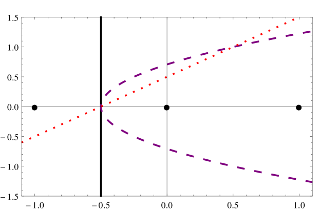
So, we can test numerically some basic ideas connected with contour deformations. Let us parameterize integral Eq. (6) as

$$z=\Re[z]+i\;t,~{}~{}~{}t\in(-\infty,+\infty)$$ (8)

where $\Re[z]$ is chosen in three different ways (see Fig. 1):

$$z(t)=x_{0}+it~{}:~{}~{}~{}~{}V_{-1}^{C_{1}}(s) = \int_{-\infty}^{+\infty}(i)~{}dt~{}J[z(t)],$$ (9)

$$z(t)=x_{0}+{\bf{\theta}}t+it~{}:~{}~{}~{}~{}V_{-1}^{C_{2}}(s) = \int_{-\infty}^{+\infty}({\bf{\theta}}+i)~{}dt~{}J[z(t)],$$ (10)

$$z(t)=x_{0}+at^{2}+it~{}:~{}~{}~{}~{}V_{-1}^{C_{3}}(s) = \int_{-\infty}^{+\infty}(2at+i)~{}dt~{}J[z(t)].$$ (11)

Figure 1: Integration contours chosen for the real part of the complex variable $z$ defined in Eqs. (6),(8) and Eqs. (9)-(11). For $C_{2}$ $\alpha=\arctan(\frac{1}{\theta})$. Deformation from $C_{1}$ to $C_{2}$ or $C_{3}$ does not cross poles (black dots).

The accuracy of the results of integration at some Minkowskian point depends strongly on the chosen contour. For instance, taken $s=2$, Eq. (7) gives an exact result (which is purely real)

$$V_{-1}(2)|_{\text{analyt.}} = \frac{\pi}{4}={0.785398163}39744830962.$$ (12)

If we try to find a numerical solution directly to the integral Eq. (6) by trying to control oscillatory behavior of the integrand using special algorithms, like the Pantis method, as in [20], the obtained result estimated this way is $V_{-1}(2)|_{\text{Pantis}}^{MB.m}=0.7925-{0.0225\;i}$. It is obviously not an acceptable result for further use.

Let us estimate the result using contours $C_{1},C_{2},C_{3}$. We get

$$V_{-1}(2)|_{\text{$C_{1}$ }} = 4.4574554985139977188+{4.5139812364645122275\;i}$$ (13)

$$V_{-1}(2)|_{\text{$C_{2}$}} = {0.785398163}3859819-5.420140575251864\cdot{10^{-15}}\;i$$ (14)

$$V_{-1}(2)|_{\text{$C_{3}$}} = {0.785398163}2958756+2.435551760271437\cdot{10^{-15}}\;i.$$ (15)

As we can see, taking countours $C_{2}$ and $C_{3}$ and comparing numerical results with Eq. (12), already 10-12 digits of accuracy for the integration can be obtained. Similar accuracy can be obtained for other points in the Minkowskian region above the second threshold, $s>4$.

3.2 Basic methods and tricks for accurate numerical integrations

We experienced three main methods to integrate efficiently MB integrals, namely

• Specific integration methods for oscillating integrands;

• Integration contour deformations;

• Integration contour shifts.

As discussed and shown in the last section, method I is not effective for numerical treatment of MB integrals in physical regions (and it is known that it is a complicated issue, see for instance [65]) and the method II is limited, though it may be quite effective for 1-dimensional cases.

Method III is new, and as will be shown, it is an effective and programmable method, even for numerical calculation of multi-dimensional MB integrals.

Method III. The idea.

The idea of contour shifts is rather plain and straigthforward. Imagine we have some MB integral with fixed real parts of complex integration variables $z_{i}$ (as it is usually the case, such MB representations are available using AMBRE and MB.m). We then shift one or more variables $z_{i}$ by multiply integer numbers. By virtue of Gamma functions and kinematics involved, a new, ”shifted” MB integral is obtained, plus a bunch of residue integrals from controlled crossing of poles. The aim is to get a shifted original integral whose absolute magnitude, by virtue of applied shifts, is smaller and smaller. How far we go with shifts (so going down in magnitude of the original MB integral) depends on which accuracy of the final numerical result we aim at. The remaining residue MB subintegrals after shifts are of lower MB dimension. The procedure is iterative. In a next step MB residue integrals of lower MB dimensions can be treated the same way. When a procedure is terminated depends on the accuracy of the generated residue MB integrals and on the desired accuracy for the original MB integral. In passing, there can be large numerical cancellations among numerically equal subintegrals of different sign, which must be also controlled properly.

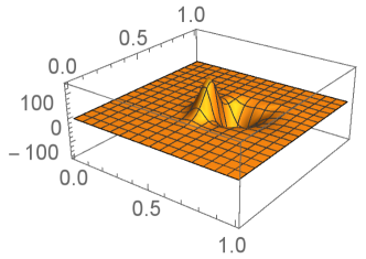
As an illustrative example of the efficiency of shifts, let us take the two-dimensional integrand

$$J(z_{1},z_{2})=\frac{2(-\mathrm{\frac{s}{M_{Z}^{2}}})^{-z_{1}-z_{2}}\Gamma[-1-z_{1}-2z_{2}]\Gamma[-z_{1}-z_{2}]\Gamma[-z_{2}]\Gamma[1+z_{2}]^{3}\Gamma[1+z_{1}+z_{2}]}{\mathrm{s^{2}}\Gamma[1-z_{1}]}$$ (16)

and start with the contour of integration $C_{1}$, Eq. (9), where $\Re{[z_{1}]}=z_{10}=0,\;\Re{[z_{2}]}=z_{20}=-0.7$. It is interesting to note that at the the kinematic point $s/M_{Z}^{2}=1+i\varepsilon$ ($\varepsilon$ is an arbitrarily small parameter chosing the correct sheet), which is a point explored in the $Z\to bb$ studies [58, 59], shifts works well. To see this, we shift $z_{2}$ variable, $z_{2}=z_{20}+n$. The integral is now a discrete function of the number of shifts ${n}$:

$$I^{C_{1}}(s,M_{Z},{n})=\int\limits_{-\infty}^{+\infty}\int\limits_{-\infty}^{+\infty}(i)^{2}J(z_{10}+it_{1},z_{20}+{n}+it_{2})\mathrm{d}t_{1}\mathrm{d}t_{2}.$$ (17)

Using Stirling’s formula

$$\Gamma(z)=\sqrt{2\pi}~{}e^{-z}~{}z^{z-1/2}\left(1+\frac{1}{12z}+\frac{1}{288z^{2}}-\frac{139}{51840z^{3}}-\frac{571}{2488320z^{4}}+\cdots\right)$$ (18)

and the relation $\ln(-|R|)\to\ln(-|R|\pm i\epsilon)=\ln(|R|)\pm{i~{}\pi}$ the worst asymptotic behavior for the integrand is for $t_{1}\rightarrow-\infty,\;t_{2}\rightarrow 0$:

$$J(z_{10}+it_{1},z_{20}+{n}+it_{2})\simeq t_{1}^{-2-2(z_{20}+n)}.$$ (19)

For $n=0$ and $z_{20}=-0.7$, the integrand $J(z_{1},z_{2})$ drops off like $t_{1}^{-0.6}$. This slow convergence is similar to the QED massive vertex, discussed above. However, increasing $n$, the module of the integrand becomes smaller, making possible to get it arbitrarily small, see Fig. 2.

Figure 2: Module of real part of the integral $I^{C_{1}}(s,M_{Z},{n})$ as a function of $n$.

We can see that the shifts improve the asymptotic behavior and reduce the order of magnitude of the integral $I^{C_{1}}(s,M_{Z},{n})$. The absolute and the module of an imaginary part of $I^{C_{1}}(s,M_{Z},{n})$ behave similarly.

Automatic algorithms for finding the suitable shifts and contour deformations are implemented in MBnumerics.m [64]. At the moment an effective strategy is: Starting from original $n-$dimensional MB integrals, MBnumerics.m looks for well converging $n-1$ and $n-2$ integrals, and remaining $n-$dimensional integrals. Up to 4-dimensional integrals, the deterministic Cuhre method of the CUBA package [66, 67] can be used. In this way accuracy of calculation can be controlled.

At the moment it appears that linear contour deformations as in Eq. (10) are sufficient (in [25, 52] they are called contour rotations) for the evaluation of shifted and residue integrals, when merged with another trick, namely mapping of variables in integrands. Contour $C_{3}$ is the basic contour used for an evaluation of 1-dim integrals.

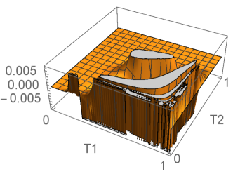
Mapping of variables is necessary, making possible the numerical integration of integrals over finite regions. At the same time the numerical stability of integrations is improved. In [20] a logarithmic mapping has been used

$$z_{i} = x_{i}+i\ln\left(\frac{t_{i}}{1-t_{i}}\right),~{}~{}t_{i}\in(0,1),\;\;\;{\rm Jacobian}:\;\;J_{i}(t_{i})=\frac{1}{t_{i}(1-t_{i})}.$$ (20)

Unfortunately, the curvature rules of Cuhre cannot approximate integrands with a power law $1/t_{i}$ behaviour, which is exactly what may happen at the boundaries of the unit hypercube, due to the Jacobians (20). An example for such a problematic integral defined in Eq. (21) is given in Fig. 3.

$$I=\int\limits_{-\frac{1}{3}-i\infty}^{-\frac{1}{3}+i\infty}dz_{1}\int\limits_{-\frac{2}{3}-i\infty}^{-\frac{2}{3}+i\infty}dz_{2}\left(\frac{-s}{M_{Z}^{2}}\right)^{-z_{1}}\frac{\Gamma[-z_{1}]^{3}\Gamma[1+z_{1}]\Gamma[z_{1}-z_{2}]\Gamma[-z_{2}]^{3}\Gamma[1+z_{2}]\Gamma[1-z_{1}+z_{2}]}{s~{}~{}\Gamma[1-z_{1}]^{2}\Gamma[-z_{1}-z_{2}]\Gamma[1+z_{1}-z_{2}]}$$ (21)

Figure 3: Logarithmic mapping for the integrand in Eq. (21) . On left (right) real (imaginary) part of the integral is given.

Instead of a logarithmic, a tangent mapping is used in MBnumerics.m:

$$z_{i} = x_{i}+i~{}\frac{1}{\tan(-\pi t_{i})},~{}~{}t_{i}\in(0,1),\;\;\;{\rm Jacobian}:\;\;J_{i}=\frac{\pi}{\sin^{2}{[(\pi t_{i})]}}.$$

Figure 4: Tangent mapping for the integrand in Eq. (21) . On left (right) real (imaginary) part of the integral is given.

Comparing Fig. 3 and Fig. 4, even with naked eye one can see that tangent mapping does not give boundary instabilities and the integrand is relatively smooth. To improve the stability of numerical integrations further, in addition, $\Pi_{i}\;\Gamma_{i}\to e^{\sum_{i}\ln\Gamma_{i}}$ transformation helps considerable.

As already said, shifts come with mappings and contour deformations and MBnumerics.m uses linear contour deformations (rotations), Eq. (10). The point is that a linear change of variables introduces an additional exponential factor which, chosen properly, may help to damp integrand oscillations. Using this transformation no poles of Gamma functions are crossed as the rotation is applied to all MB integration variables at once, first noted in [52]. To see how to choose the rotation parameter properly to get damping factors, let us consider the asymptotic behaviour of the integral Eq. (6) using Eq. (18).
Part I in Eq. (6) for the contour $C_{1}$ gives

$$(-s)^{-(x_{0}+it)}=(s)^{-(x_{0}+it)}(-1-i\epsilon)^{-(x_{0}+it)}=(s)^{-(x_{0}+it)}e^{i\pi x_{0}}{e^{-\pi t}}.$$ (22)

We can see that if ${t\to-\infty}$ the last exponential factor explodes. Fortunately, from Part II of Eq. (6), we get

$$\Re\left[\frac{\Gamma^{3}[-x_{0}-it]\Gamma[x_{0}+it]}{\Gamma[2(x_{0}+it)]}\right]\simeq 2\pi^{3/2}\sqrt{\left|\frac{s}{t}\right|}e^{-\pi|t|}.$$ (23)

The numerator cancels out an exponential factor in Eq. (22), though the badly convergent part $t^{-1/2}$ remains. It can be stabilized further by rotating the $z$ variable by some angle $\alpha(\theta)$, see Fig. 1

$$z=x_{0}+it\to x_{0}+(\theta+i)t.$$ (24)

Now, the complete result for Eq. (6) can be cast in the following way

$$\Re\left[\lim\limits_{|z|\to\infty}V_{-1}(s)\right]\sim 2\pi^{3/2}\sqrt[4]{\theta^{2}+1}\sqrt{\left|\frac{s}{t}\right|}e^{-\pi\left|t\right|+t\arg(-s)+\theta t\log\left(\frac{4}{s}\right)},\;\;s=\Re[s]+i\varepsilon,$$ (25)

where

$$\arg(-s)=\begin{cases}-\pi,&\Re[s]>0,\\ -\pi/2,&\Re[s]=0,\\ 0,&\Re[s]<0,\end{cases}$$ (26)

It can be seen easily that for any value of the kinematical variable $s\neq 4$ and $s\neq 0$ the $\theta$ parameter can be chosen to make the real part of the exponents argument negative, for instance, for $s=1+i\varepsilon$ the condition is

$$0<\theta<\frac{\pi}{\log(2)}.$$ (27)

Let us look for some more complicated, two-dimensional example of contour deformations:

$$J(z_{1},z_{2})=\frac{\left(\frac{M_{W}^{2}}{M_{T}^{2}}\right)^{z_{2}}s^{2}\left(-\frac{s}{M_{T}^{2}}\right)^{z_{1}-z_{2}}\Gamma[-z_{1}]\Gamma[z_{1}]\Gamma[2-z_{2}]\Gamma[4+z_{1}-z_{2}]\Gamma[z_{2}]\Gamma[-z_{2}])}{4M_{T}^{4}\Gamma[6+z_{1}-2z_{2}]}.$$ (28)

The integral will be integrated over $C_{1}$:

$$K^{C_{1}}(s,M_{W},M_{T})=\int\limits_{-\infty}^{+\infty}\int\limits_{-\infty}^{+\infty}(i)^{2}J(z_{10}+it_{1},z_{20}+it_{2})\mathrm{d}t_{1}\mathrm{d}t_{2},\;\;z_{10}=0.7,\;z_{20}=-1.2,$$ (29)

and over $C_{2}$:

$$K^{C_{2}}(s,M_{W},M_{T})=\int\limits_{-\infty}^{+\infty}\int\limits_{-\infty}^{+\infty}(i+{\color[rgb]{0,0,1}\theta})^{2}J(z_{10}+(i+{\color[rgb]{0,0,1}\theta})t_{1},z_{20}+(i+{\color[rgb]{0,0,1}\theta})t_{2})\mathrm{d}t_{1}\mathrm{d}t_{2},\;\;z_{10}=0.7,\;z_{20}=-1.2.$$ (30)

The worst asymptotic behavior of the integrand $J^{C_{1}}$ takes place for $t_{1}\rightarrow 0,\;t_{2}\rightarrow-\infty$

$$J(z_{10}+t_{1},z_{20}+t_{2})\simeq t_{2}^{-\frac{3}{2}}.$$ (31)

Thus the integral $K^{C_{1}}$ is very slowly convergent. Taking $s=M_{Z}^{2}$ and $\theta=0.7$, the asymptotic behavior of the integrand $J^{C_{2}}$ is like in the Euclidean case and the numerical evaluation of $K^{C_{2}}$ yields honest high accuracy. In Fig. 5 real parts of the integrand $J$ evaluated over contours $C_{1}$ and $C_{2}$ are given.

Figure 5: Real part of the integrand $J$ defined in Eq.(3.22) evaluated over contours $C_{1}$ and $C_{2}$. $T_{1}$ and $T_{2}$ are integration variables due to a tangent mapping: $t_{i}=1/\tan[-\pi T_{i}]$.

3.3 MBnumerics.m, present situation

The algorithm has been applied succesfully so far to up to four-dimensional MB integrals with the desired accuracy (8 digits). In calculations, the AMBRE constructions are not the main issue as far as time of calculation is concerned. For numerical results, time consuming is the determination of optimal contours where the proper grid for threshold kinematics and the treatment of tails of integrands bother. The second time factor is connected with numerical integration over the optimal contours. To get high accuracy, the optimal strategy is to treat MB integrals with maximal four dimensions, and to use Cuhre, which is not a Monte Carlo, but a deterministic algorithm [67]. A decent precision can be obtained in this way. For some specific cases MB integrals have been initially reduced using KIRA package [68], followed by their numerical evaluation with MBnumerics.m.

Finally, we give as another example the constant part of the 3-dimensional integrand Eq. (32) drawn in Fig. 6

$$(-s)^{-2{\epsilon}-{z_{2}}-2}\left(m^{2}\right)^{{z_{2}}}\Gamma[-{\epsilon}]\Gamma[-{z_{1}}]\Gamma[-{z_{2}}]\Gamma[-{z_{3}}]\Gamma^{2}[{z_{3}}+1]\Gamma[-{\epsilon}-{z_{1}}]\Gamma[-{\epsilon}-{z_{2}}]\Gamma[{z_{1}}+{z_{3}}+1]$$

$$\times\frac{\Gamma[-2{\epsilon}-{z_{1}}-{z_{3}}-1]\Gamma[-2{\epsilon}-{z_{2}}-{z_{3}}-1]\Gamma[-2{\epsilon}-{z_{1}}-{z_{2}}-{z_{3}}-1]\Gamma[2{\epsilon}+{z_{1}}+{z_{2}}+{z_{3}}+2]}{\Gamma[-2{\epsilon}-{z_{1}}]\Gamma[-3{\epsilon}-{z_{2}}]\Gamma[-2{\epsilon}-{z_{2}}]\Gamma[-2{\epsilon}-{z_{1}}-{z_{2}}]},$$

(32)

which shows how powerful MBnumerics.m can be.

Figure 6: Non-planar vertex with one massive crossed line. Figure generated by PlanarityTest [19, 18].

In this case, results obtained with different available methods and programs in the Euclidean region are the following, $-(p_{1}+p_{2})^{2}=m^{2}=1$:

$$\begin{array}[]{ll}{\rm Analytical}:&-0.4966198306057021\\ {\rm MB(Vegas)}:&-0.4969417442183914\\ {\rm MB(Cuhre)}:&-0.4966198313219404\\ {\rm FIESTA}:&-0.4966184488196595\\ {\rm SecDec}:&-0.4966192150541896\end{array}$$

For the Minkowskian region, $(p_{1}+p_{2})^{2}=m^{2}=1+i\varepsilon$, constant part:

$$\begin{array}[]{lc}{\rm Analytical}:&-{0.778599608}979684-{4.123512}593396311\cdot i\\ {\rm MBnumerics}:&-{0.778599608}324769-{4.123512}600516016\cdot i\\ {\rm MB(Vegas)}:&{\rm big\;error}\\ {\rm MB(Cuhre)}:&{\rm NaN}\\ {\rm FIESTA}:&{\rm big\;error}\\ {\rm SecDec}:&{\rm big\;error}\end{array}$$

For more examples and comparisons, see [58, 69].

4 Summary

We have summarized the present status of the AMBRE project for the construction of MB integrals. New versions of the package for planar and non-planar integrals are given.

The new package MBnumerics.m has been discussed in which MB integrals can be evaluated numerically in a Minkowskian region. Oscillatory behaviour of MB integrals is treated by shifts of variables, stabilility of integrals is further improved by contour deformations and mapping of variables. Shifts of contours are so powerful that sometimes the method alone is sufficient to obtain high accuracy. Difficult cases like thresholds are also treatable now. For $Z\to bb$, MBnumerics.m turned out to be a very strong and effective tool [58, 59].

References

- [1] R. H. Mellin, Om definita integraler, Acta Soc. Sci. Fenn. 20(7), 1 (1895).
- [2] E. W. Barnes, The theory of the gamma function, Messenger Math. 29(2), 64 (1900).
- [3] V. Smirnov, Evaluating Feynman integrals, Springer Tracts Mod. Phys. 211 (2004) 1–244.
- [4] J. Gluza, K. Kajda, T. Riemann, AMBRE - a Mathematica package for the construction of Mellin-Barnes representations for Feynman integrals, Comput. Phys. Commun. 177 (2007) 879–893. cmttcmttcmttcmttarXiv:0704.2423, cmttcmttcmttcmttdoi:10.1016/j.cpc.2007.07.001.
- [5] J. D. Bjorken, T. T. Wu, Perturbation Theory of Scattering Amplitudes at High Energies, Phys. Rev. 130 (1963) 2566–2572. cmttcmttcmttcmttdoi:10.1103/PhysRev.130.2566.
- [6] M. C. Bergere, Y.-M. P. Lam, Asymptotic expansion of Feynman amplitudes. Part 1: The convergent case, Commun. Math. Phys. 39 (1974) 1. cmttcmttcmttcmttdoi:10.1007/BF01609168.
- [7] N.I. Ussyukina, On a Representation for Three Point Function, Teor.Mat.Fiz. 22, 300 (1975).
- [8] E. Boos, A. I. Davydychev, A Method of evaluating massive Feynman integrals, Theor.Math.Phys. 89 (1991) 1052–1063. cmttcmttcmttcmttdoi:10.1007/BF01016805.
- [9] A. I. Davydychev, Recursive algorithm of evaluating vertex type Feynman integrals, J.Phys. A25 (1992) 5587–5596.
- [10] N. I. Usyukina, A. I. Davydychev, Exact results for three and four point ladder diagrams with an arbitrary number of rungs, Phys. Lett. B305 (1993) 136–143. cmttcmttcmttcmttdoi:10.1016/0370-2693(93)91118-7.
- [11] V. A. Smirnov, Analytical result for dimensionally regularized massless on shell double box, Phys. Lett. B460 (1999) 397–404. cmttcmttcmttcmttarXiv:hep-ph/9905323, cmttcmttcmttcmttdoi:10.1016/S0370-2693(99)00777-7.
- [12] J. Tausk, Nonplanar massless two loop Feynman diagrams with four on-shell legs, Phys. Lett. B469 (1999) 225–234. cmttcmttcmttcmttarXiv:hep-ph/9909506, cmttcmttcmttcmttdoi:10.1016/S0370-2693(99)01277-0.
- [13] M. Czakon (MB, MBasymptotics), D. Kosower (barnesroutines), A. Smirnov, V. Smirnov (MBresolve), K. Bielas, I. Dubovyk, J. Gluza, K. Kajda, T. Riemann (AMBRE, PlanarityTest), MBtools webpage, https://mbtools.hepforge.org/.
- [14] J. Gluza, K. Kajda, T. Riemann, V. Yundin, Numerical Evaluation of Tensor Feynman Integrals in Euclidean Kinematics, Eur. Phys. J. C71 (2011) 1516. cmttcmttcmttcmttarXiv:1010.1667, cmttcmttcmttcmttdoi:10.1140/epjc/s10052-010-1516-y.
- [15] U. of Silesia, Katowice, webpage http://prac.us.edu.pl/~gluza/ambre.
- [16] J. Blümlein, I. Dubovyk, J. Gluza, M. Ochman, C. G. Raab, et al., Non-planar Feynman integrals, Mellin-Barnes representations, multiple sums, PoS LL2014 (2014) 052. cmttcmttcmttcmttarXiv:1407.7832.
- [17] I. Dubovyk, J. Gluza, T. Riemann, Non-planar Feynman diagrams and Mellin-Barnes representations with , J. Phys. Conf. Ser. 608 (2015) 012070. DESY 14–174 (13 April 2016). cmttcmttcmttcmttdoi:10.1088/1742-6596/608/1/012070.
- [18] K. Bielas, I. Dubovyk, PlanarityTest.m, a Mathematica package for testing the planarity of Feynman diagrams, http://us.edu.pl/~gluza/ambre/planarity/.
- [19] K. Bielas, I. Dubovyk, J. Gluza, T. Riemann, Some Remarks on Non-planar Feynman Diagrams, Acta Phys. Polon. B44 (2013) 2249–2255. cmttcmttcmttcmttarXiv:1312.5603, cmttcmttcmttcmttdoi:10.5506/APhysPolB.44.2249.
- [20] M. Czakon, Automatized analytic continuation of Mellin-Barnes integrals, Comput. Phys. Commun. 175 (2006) 559–571. cmttcmttcmttcmttarXiv:hep-ph/0511200, cmttcmttcmttcmttdoi:10.1016/j.cpc.2006.07.002.
- [21] A. Smirnov, V. Smirnov, On the Resolution of Singularities of Multiple Mellin-Barnes Integrals, Eur. Phys. J. C62 (2009) 445–449. cmttcmttcmttcmttarXiv:0901.0386, cmttcmttcmttcmttdoi:10.1140/epjc/s10052-009-1039-6.
- [22] M. Ochman, T. Riemann, MBsums - a Mathematica package for the representation of Mellin-Barnes integrals by multiple sums, Acta Phys. Polon. B46 (2015) 2117. cmttcmttcmttcmttarXiv:1511.01323, cmttcmttcmttcmttdoi:10.5506/APhysPolB.46.2117.
- [23] S. Friot, D. Greynat, On convergent series representations of Mellin-Barnes integrals, J. Math. Phys. 53 (2012) 023508. cmttcmttcmttcmttarXiv:1107.0328, cmttcmttcmttcmttdoi:10.1063/1.3679686.
- [24] C. Anastasiou, A. Daleo, Numerical evaluation of loop integrals, JHEP 0610 (2006) 031. cmttcmttcmttcmttarXiv:hep-ph/0511176, cmttcmttcmttcmttdoi:10.1088/1126-6708/2006/10/031.
- [25] A. Freitas, Numerical multi-loop integrals and applicationscmttcmttcmttcmttarXiv:1604.00406.
- [26] T. Hahn, Generating Feynman diagrams and amplitudes with FeynArts 3, Comput. Phys. Commun. 140 (2001) 418–431. cmttcmttcmttcmttarXiv:hep-ph/0012260.
- [27] B. Chokoufe Nejad, T. Hahn, J. N. Lang, E. Mirabella, FormCalc 8: Better Algebra and Vectorization, J. Phys. Conf. Ser. 523 (2014) 012050. cmttcmttcmttcmttarXiv:1310.0274, cmttcmttcmttcmttdoi:10.1088/1742-6596/523/1/012050.
- [28] G. Ossola, C. G. Papadopoulos, R. Pittau, CutTools: A Program implementing the OPP reduction method to compute one-loop amplitudes, JHEP 03 (2008) 042. cmttcmttcmttcmttarXiv:0711.3596, cmttcmttcmttcmttdoi:10.1088/1126-6708/2008/03/042.
- [29] C. F. Berger, Z. Bern, L. J. Dixon, F. Febres Cordero, D. Forde, H. Ita, D. A. Kosower, D. Maitre, An Automated Implementation of On-Shell Methods for One-Loop Amplitudes, Phys. Rev. D78 (2008) 036003. cmttcmttcmttcmttarXiv:0803.4180, cmttcmttcmttcmttdoi:10.1103/PhysRevD.78.036003.
- [30] A. van Hameren, C. G. Papadopoulos, R. Pittau, Automated one-loop calculations: A Proof of concept, JHEP 09 (2009) 106. cmttcmttcmttcmttarXiv:0903.4665, cmttcmttcmttcmttdoi:10.1088/1126-6708/2009/09/106.
- [31] S. Badger, B. Biedermann, P. Uwer, NGluon: A Package to Calculate One-loop Multi-gluon Amplitudes, Comput. Phys. Commun. 182 (2011) 1674–1692. cmttcmttcmttcmttarXiv:1011.2900, cmttcmttcmttcmttdoi:10.1016/j.cpc.2011.04.008.
- [32] P. Mastrolia, G. Ossola, T. Reiter, F. Tramontano, Scattering AMplitudes from Unitarity-based Reduction Algorithm at the Integrand-level, JHEP 08 (2010) 080. cmttcmttcmttcmttarXiv:1006.0710, cmttcmttcmttcmttdoi:10.1007/JHEP08(2010)080.
- [33] V. Hirschi, R. Frederix, S. Frixione, M. V. Garzelli, F. Maltoni, R. Pittau, Automation of one-loop QCD corrections, JHEP 05 (2011) 044. cmttcmttcmttcmttarXiv:1103.0621, cmttcmttcmttcmttdoi:10.1007/JHEP05(2011)044.
- [34] G. Cullen, et al., Golem95C: A library for one-loop integrals with complex masses, Comput. Phys. Commun. 182 (2011) 2276–2284. cmttcmttcmttcmttarXiv:1101.5595, cmttcmttcmttcmttdoi:10.1016/j.cpc.2011.05.015.
- [35] G. Cullen, N. Greiner, G. Heinrich, G. Luisoni, P. Mastrolia, G. Ossola, T. Reiter, F. Tramontano, Automated One-Loop Calculations with GoSam, Eur. Phys. J. C72 (2012) 1889. cmttcmttcmttcmttarXiv:1111.2034, cmttcmttcmttcmttdoi:10.1140/epjc/s10052-012-1889-1.
- [36] J. Fleischer, T. Riemann, V. Yundin, New developments in PJFry, PoS LL2012 (2012) 020, http://pos.sissa.it/…151/020/LL2012_020.pdf. cmttcmttcmttcmttarXiv:1210.4095.
- [37] F. Cascioli, P. Maierhofer, S. Pozzorini, Scattering Amplitudes with Open Loops. cmttcmttcmttcmttarXiv:hep-ph/1111.5206.
- [38] G. van Oldenborgh, FF: A Package to evaluate one loop Feynman diagrams, Comput. Phys. Commun. 66 (1991) 1–15. cmttcmttcmttcmttdoi:10.1016/0010-4655(91)90002-3.
- [39] A. van Hameren, OneLOop: For the evaluation of one-loop scalar functions, Comput. Phys. Commun. 182 (2011) 2427–2438. cmttcmttcmttcmttarXiv:1007.4716, cmttcmttcmttcmttdoi:10.1016/j.cpc.2011.06.011.
- [40] R. K. Ellis, G. Zanderighi, Scalar one-loop integrals for QCD, JHEP 02 (2008) 002. cmttcmttcmttcmttarXiv:0712.1851, cmttcmttcmttcmttdoi:10.1088/1126-6708/2008/02/002.
- [41] A. Denner, S. Dittmaier, L. Hofer, Collier: a fortran-based Complex One-Loop LIbrary in Extended Regularizations, cmttcmttcmttcmttarXiv:1604.06792.
- [42] A. V. Smirnov, FIESTA 4: optimized Feynman integral calculations with GPU support, cmttcmttcmttcmttarXiv:1511.03614.
- [43] S. Borowka, G. Heinrich, S. P. Jones, M. Kerner, J. Schlenk, T. Zirke, SecDec 3.0: numerical evaluation of multi-scale integrals beyond one loop, Comput. Phys. Commun. 196 (2015) 470–491. cmttcmttcmttcmttarXiv:1502.06595, cmttcmttcmttcmttdoi:10.1016/j.cpc.2015.05.022.
- [44] A. Freitas, Numerical evaluation of multi-loop integrals using subtraction terms, JHEP 1207 (2012) 132. cmttcmttcmttcmttarXiv:1205.3515, cmttcmttcmttcmttdoi:10.1007/JHEP07(2012)132,10.1007/JHEP09(2012)129.
- [45] S. P. Martin, D. G. Robertson, TSIL: A Program for the calculation of two-loop self-energy integrals, Comput. Phys. Commun. 174 (2006) 133–151. cmttcmttcmttcmttarXiv:hep-ph/0501132, cmttcmttcmttcmttdoi:10.1016/j.cpc.2005.08.005.
- [46] M. Caffo, H. Czyz, M. Gunia, E. Remiddi, BOKASUN: A Fast and precise numerical program to calculate the Master Integrals of the two-loop sunrise diagrams, Comput. Phys. Commun. 180 (2009) 427–430. cmttcmttcmttcmttarXiv:0807.1959, cmttcmttcmttcmttdoi:10.1016/j.cpc.2008.10.011.
- [47] A. Ghinculov, J. van der Bij, Massive two loop diagrams: The Higgs propagator, Nucl. Phys. B436 (1995) 30–48. cmttcmttcmttcmttarXiv:hep-ph/9405418.
- [48] A. Ghinculov, Y.-P. Yao, Massive two-loop integrals in renormalizable theories, Nucl. Phys. B516 (1998) 385–401. cmttcmttcmttcmttarXiv:hep-ph/9702266.
- [49] S. Becker, S. Weinzierl, Direct contour deformation with arbitrary masses in the loop, Phys. Rev. D86 (2012) 074009. cmttcmttcmttcmttarXiv:1208.4088, cmttcmttcmttcmttdoi:10.1103/PhysRevD.86.074009.
- [50] S. Becker, S. Weinzierl, Direct numerical integration for multi-loop integrals, Eur. Phys. J. C73 (2) (2013) 2321. cmttcmttcmttcmttarXiv:1211.0509, cmttcmttcmttcmttdoi:10.1140/epjc/s10052-013-2321-1.
- [51] G. Passarino, An Approach toward the numerical evaluation of multiloop Feynman diagrams, Nucl. Phys. B619 (2001) 257–312. cmttcmttcmttcmttarXiv:hep-ph/0108252, cmttcmttcmttcmttdoi:10.1016/S0550-3213(01)00528-4.
- [52] A. Freitas, Y.-C. Huang, On the Numerical Evaluation of Loop Integrals With Mellin-Barnes Representations, JHEP 04 (2010) 074. cmttcmttcmttcmttarXiv:1001.3243, cmttcmttcmttcmttdoi:10.1007/JHEP04(2010)074.
- [53] A. Freitas, Y.-C. Huang, Electroweak two-loop corrections to and using numerical Mellin-Barnes integrals, JHEP 1208 (2012) 050. cmttcmttcmttcmttarXiv:1205.0299, cmttcmttcmttcmttdoi:10.1007/JHEP08(2012)050.
-
[54]
Z. Peng, Topics in N = 4
Yang-Mills theory, Ph.D. thesis, IPhT, Saclay (2012).
URL http://tel.archives-ouvertes.fr/tel-00834200 - [55] G. Somogyi, Angular integrals in d dimensions, J. Math. Phys. 52 (2011) 083501. cmttcmttcmttcmttarXiv:1101.3557, cmttcmttcmttcmttdoi:10.1063/1.3615515.
- [56] C. Anastasiou, S. Beerli, A. Daleo, Evaluating multi-loop Feynman diagrams with infrared and threshold singularities numerically, JHEP 0705 (2007) 071. cmttcmttcmttcmttarXiv:hep-ph/0703282, cmttcmttcmttcmttdoi:10.1088/1126-6708/2007/05/071.
- [57] C. Anastasiou, C. Duhr, F. Dulat, B. Mistlberger, Soft triple-real radiation for Higgs production at N3LO, JHEP 07 (2013) 003. cmttcmttcmttcmttarXiv:1302.4379, cmttcmttcmttcmttdoi:10.1007/JHEP07(2013)003.
[58]
I. Dubovyk, A. Freitas, J. Gluza, T. Riemann, J. Usovitsch, “30 years, 715
integrals, and 1 dessert, or: Bosonic contributions to the 2-loop Zbb
vertex”, talk by T. Riemann at LL2016, 24-28 April 2016, Leipzig, Germany,
to appear in the proceedings.
https://indico.desy.de/getFile.py/access?contribId=63&sessionId=12&resI%d=0&materialId=slides&confId=12010. - [59] I. Dubovyk, A. Freitas, J. Gluza, T. Riemann and J. Usovitsch, “The two-loop electroweak bosonic corrections to ”, arXiv:1607.08375 [hep-ph].
- [60] M. Czakon, J. Gluza, T. Riemann, Master integrals for massive two-loop bhabha scattering in QED, Phys. Rev. D71 (2005) 073009. cmttcmttcmttcmttarXiv:hep-ph/0412164, cmttcmttcmttcmttdoi:10.1103/PhysRevD.71.073009.
- [61] M. Czakon, J. Gluza, T. Riemann, The Planar four-point master integrals for massive two-loop Bhabha scattering, Nucl. Phys. B751 (2006) 1–17. cmttcmttcmttcmttarXiv:hep-ph/0604101, cmttcmttcmttcmttdoi:10.1016/j.nuclphysb.2006.05.033.
- [62] S. Actis, M. Czakon, J. Gluza, T. Riemann, Virtual hadronic and leptonic contributions to Bhabha scattering, Phys. Rev. Lett. 100 (2008) 131602. cmttcmttcmttcmttarXiv:0711.3847, cmttcmttcmttcmttdoi:10.1103/PhysRevLett.100.131602.
- [63] S. Actis, M. Czakon, J. Gluza, T. Riemann, Virtual Hadronic and Heavy-Fermion Corrections to Bhabha Scattering, Phys. Rev. D78 (2008) 085019. cmttcmttcmttcmttarXiv:0807.4691, cmttcmttcmttcmttdoi:10.1103/PhysRevD.78.085019.
- [64] I. Dubovyk, T. Riemann and J. Usovitsch, MBnumerics.m 1.0, a Mathematica package for numerical evaluation of Mellin-Barnes integrals in Minkowskian regions, in preparation.
- [65] D. H. Bailey, J. M. Borwein, Hand-to-hand combat with thousand-digit integrals, J. Comput. Science 3 (2012) 77–86.
- [66] T. Hahn, CUBA: A library for multidimensional numerical integration, Comput. Phys. Commun. 168 (2005) 78–95. cmttcmttcmttcmttarXiv:hep-ph/0404043, cmttcmttcmttcmttdoi:10.1016/j.cpc.2005.01.010.
- [67] T. Hahn, webpage http://www.feynarts.de/cuba/.
- [68] P. Maierhöfer, J. Usovitsch, P. Uwer, Kira 1.0, a C++ program for the reduction of Feynman integrals to masters, in preparation.
- [69] I. Dubovyk, A. Freitas, J. Gluza, T. Riemann, J. Usovitsch, to be published.