Time-varying Formation Tracking of Multiple Manipulators via Distributed Finite-time Control

Abstract

Comparing with traditional fixed formation for a group of dynamical systems, time-varying formation can produce the following benefits: i) covering the greater part of complex environments; ii) collision avoidance. This paper studies the time-varying formation tracking for multiple manipulator systems (MMSs) under fixed and switching directed graphs with a dynamic leader, whose acceleration cannot change too fast. An explicit mathematical formulation of time-varying formation is developed based on the related practical applications. A class of extended inverse dynamics control algorithms combining with distributed sliding-mode estimators are developed to address the aforementioned problem. By invoking finite-time stability arguments, several novel criteria (including sufficient criteria, necessary and sufficient criteria) for global finite-time stability of MMSs are established. Finally, numerical experiments are presented to verify the effectiveness of the theoretical results.

Keywords time-varying formation tracking, dynamic leader, multiple manipulator systems (MMSs), finite-time stability.

1 Introduction

Recently, distributed control problems for a group of dynamical systems have attracted much attentions due to its wide applications, including coordination for multi-agent systems [1]-[5], synchronization in complex networks [6, 7], distributed computing in sensor networks [8]-[10], multi-fingered hand grasping and manipulation [11, 12]. Formation control is a significant issue in the distributed control field. A formation is defined as a special configuration ($i.e.$, desired positions and orientations) formed by a cluster of interconnected autonomous agents, in which a global goal is achieved cooperatively [13]. Many formation control methods have been developed, such as virtual structure methods [14], behavior-based methods [15, 16], leader-follower methods [17], artificial potential field methods [18]. The aforementioned methods can only produce fixed formations for multi-agent systems. However, in a number of real-world applications, the formation of multi-agent systems is always changing to adapt to the dynamical changing environment. It follows that the fixed formations cannot satisfy the practical requirements of many real-world applications. It thus motivates several research on time-varying formations. Time-varying formation control algorithms for a group of unmanned aerial vehicles with its applications to quadrotor swarm systems had been presented based on consensus theory [19]. Coherent formation control of a set of agents, including unmanned aerial vehicles and unmanned ground vehicles, in the presence of time-varying formation had been studied in [20]. Time-varying formation implies that the formation of a multi-agent system can be changing as required without losing system stability, which products the following benefits: i) covering the greater part of complex environments; ii) collision avoidance. However, to the authors’ knowledge, the mathematical formulations of time-varying formation tracking are still not clear, which impedes the development and applications of the relative technologies.

On the other hand, networked robotic systems have been broadly studied due to their various advantages, including flexibility, adaptivity, fault tolerance, redundancy, and the possibility to invoke distributed sensing and actuation [21]. Many control algorithms for global asymptotic tracking of networked robotic systems described by Euler-Lagrange systems can be found in the literature. Adaptive control approaches are proposed to address the leader-follower and leaderless coordination problems for multi-manipulator systems based on graph theory [22, 23]. Distributed containment control had been developed for global asymptotic stability of Lagrangian networks under directed topologies containing a spanning tree [24]. Some distributed average tracking algorithms had been developed invoking extended PI control and applied to networked Euler-Lagrange systems [25]. The task-space tracking control problems of networked robotic systems under strongly connected graphs without task-space velocity measurements had been investigated [26]. In presence of kinematic and dynamic uncertainties, task-space synchronization had been addressed for multiple manipulators under strong connected graphs by invoking passivity control [27] and adaptive control [28]. All of the aforementioned control algorithms produce global asymptotic tracking of robotic manipulators, which implies that the system trajectories converge to the equilibrium as time goes to infinity. Finite-time stabilization of dynamical systems may give rise to fast transient and high-precision performances besides finite-time convergence to the equilibrium, and a lot of work has been done in the last several years [29]-[31].

Motivated by our preliminary work on distributed control [32, 33], the time-varying formation tracking of multiple manipulator systems (MMSs) is taken into account. Distributed finite control is developed to drive the centroid of the MMS to follow the leader at a distance and to achieve the desired time-varying formation of the MMS meanwhile. The main contributions are summarized as following: i) Comparing with the existing work based on multi-agent systems with single-integrator and double-integrator dynamics [21], we consider MMSs described by Euler-Lagrange systems. ii) Comparing with the existing fixed formation tracking algorithms for multi-agent system [34], we consider the time-varying formation tracking problems with a dynamic leader and present an explicit mathematical formulation of time-varying formation based on its practical characteristics. iii) Some novel estimator-based finite-time control algorithms are developed for the above time-varying formation tracking problems. For the presented control algorithms, some conditions (including sufficient conditions, necessary and sufficient conditions) are derived to guarantee the achievement of time-varying formation tracking.

The rest of this paper is organized as follows: system formulation and some preliminaries are presented in Section 2. The control algorithms and conditions of time-varying formation tracking are given in Section 3. In Section 4, the simulation results are presented. The conclusions are provided in Section 5.

2 Preliminaries

2.1 System formulation

The dynamics of the ith manipulator in the MMS is given as following [35]:

$${\mathcal{H}}_{i}(q_{i}){\ddot{q}}_{i}+{\mathcal{C}}_{i}(q_{i},\dot{q}_{i}){\dot{q}_{i}}+g_{i}(q_{i})=\tau_{i},$$ (1)

where $i\in{\mathcal{V}}=\{1,2,\cdots,n\}$, $t\in{\mathcal{J}}=[t_{0},\infty)$, $t_{0}\geq 0$ is the initial time, $q_{i},\dot{q}_{i}$ and $\ddot{q}_{i}\in{\mathbb{R}}^{m}$ are the position, velocity and acceleration vectors of generalized coordinates, ${\mathcal{H}}_{i}(q_{i})$ and ${\mathcal{C}}_{i}(q_{i},\dot{q}_{i})\in{\mathbb{R}}^{m\times m}$ are the inertia and the Coriolis/centrifugal force matrices, $g_{i}(q_{i})$ and $\tau_{i}\in{\mathbb{R}}^{m}$ denote the gravitational torque and the input torque respectively.

The leader for the MMS is given as following:

$$\left\{\begin{array}[]{lll}\dot{x}_{0}=v_{0},\\ \dot{v}_{0}=a_{0},\end{array}\right.$$

where $x_{0},v_{0},a_{0}\in{\mathbb{R}}^{m}$ are the position, velocity and acceleration vectors of generalized coordinates respectively.

We invoke a directed graph ${\mathcal{G}}=\{\mathcal{V},\mathcal{E},\mathcal{W}\}$ to describe the interaction of the MMS, where $\mathcal{V}$ denotes the node set given right after (1), $\mathcal{E}\subseteq{\mathcal{V}}^{2}$ is the edge set, $\mathcal{W}=[w_{ij}]_{n\times n}$ represents the adjacency matrix. The ith node denotes the ith manipulator in the MMS. An edge $\{j,i\}\in{\mathcal{E}}$ denotes that the ith node can access information from the jth node. The adjacency weight $w_{ij}$ is defined as $w_{ij}>0$ if $\{j,i\}\in{\mathcal{E}}$, and $w_{ij}=0$ otherwise. Besides, self-edges are not allowed in this paper, $i.e.$, $w_{ii}=0$. A directed path from the ith node to the jth node is an ordered sequence of edges $\{i_{1},i_{2}\},\{i_{2},i_{3}\},\cdots,$ in the directed graph. The neighbor set of the jth manipulator is denoted by ${{\mathcal{N}}_{i}}=\{{j\in{\mathcal{V}}~{}|~{}(j,i)\in\mathcal{E}}\}$. ${\mathcal{G}}$ is said to be undirected if and only if $\{j,i\}\in{\mathcal{E}}\Leftrightarrow\{i,j\}\in{\mathcal{E}}$, $i.e.$, $w_{ij}=w_{ji}$, $\forall i,j\in\mathcal{V}$. Throughout this paper, ${\mathcal{G}}$ is supposed to be undirected. Let $\mathcal{P}=[{p_{1}},{p_{2}},\ldots,{p_{n}}]^{T}$ be the nonnegative weight vector between the n nodes and the leader, where ${p_{i}}>0$ if the information of the leader is available to the ith node, namely, the ith node is pinned; ${p_{i}}=0$ otherwise. The Laplacian matrix ${\mathcal{L}}$ for ${\mathcal{G}}$ is defined as $l_{ii}=\sum\nolimits_{j=1}^{n}w_{ij}$ and $l_{ij}=-w_{ij},i\neq j$. Two assumptions throughout this paper are presented as following:
A1) The leader has a directed path to the nodes in the set $\mathcal{V}$ under $\mathcal{G}$ and $\mathcal{P}$;
A2) $\mathop{\sup}\nolimits_{t\in\mathcal{J}}\|\dot{a}_{0}(t)\|<\beta$, where $\|\cdot\|$ represents the Euclidean norm and $\beta$ is a positive constant.
By Assumption A2, the derivative of the acceleration $a_{0}(t)$ of the leader is bounded, which happens to be the actual characteristics of the trajectories that can be reachable by the manipulators described by Euler-Lagrange system [36].

Lemma 1.

[37] Suppose that Assumption A1 holds. $\mathcal{M}=(\mathcal{L}+diag\{\mathcal{P}\})\otimes I_{m}\in{\mathbb{R}}^{mn\times mn}$ is symmetric positive definite, where $\otimes$ denotes the Kronecker product and $I_{m}\in{\mathbb{R}}^{m\times m}$ represents the identity matrix.

2.2 Problem Statement

In a number of real-world applications, the desired formation for the MMS is required to be time-varying and switching according to task demands. In this section, the explicit mathematical definition of time-varying formation tracking is presented.

Let ${\digamma_{0-k}}=\{{{\digamma_{0}},{\digamma_{1}},\ldots,{\digamma_{k}}}\}$ be a finite set of desired formations, where $\digamma_{s}=\{\eta_{s1},\eta_{s2},\ldots,\eta_{sn}\}$ denotes the sth desired formation, $\eta_{si}\in{\mathbb{R}}^{m}$ denotes the local coordinate of the ith manipulator in the m-dimensional Euclidean space with respect to $\digamma_{s}$, $\forall s=0,1,\ldots,k$. Note that $\digamma_{s}$ becomes a desired geometric pattern in 2D plane if $m=2$. Let ${\mathcal{I}}=\{0,1,\ldots,k\}$ denote the index set of ${\digamma_{0-k}}$. A switching signal ${\sigma(t)}:\mathcal{J}\to\mathcal{I}$ is introduced with a sequence of time points $\{t_{1},t_{2},\ldots,t_{s},\ldots\}$, satisfying ${t_{0}}<{t_{1}}<\cdots<{t_{s}}<\cdots$, at which the desired formation changes. Let $\digamma(t)$ be the desired formation at time $t$. Then for any $t\in[t_{s},t_{s+1})$, the desired formation $\digamma(t)=\digamma_{\sigma(t)}=\digamma_{s}\in\digamma_{0-k}$. Besides, we assume that the desired formation is closed at each time instant, $i.e.$, $\sum\nolimits_{i=1}^{n}{{\eta_{si}}=0}$, $\forall s\in\mathcal{I}$.

The control objective is to design distributed control $\tau_{i}$ for the ith manipulator by invoking its information ($i.e.$, $q_{i}$, $\dot{q}_{i}$ and $\eta_{si}$) and its neighbour node’s states ($i.e.$, $q_{j}$, $\dot{q}_{j}$ and $\eta_{sj}$ for $j\in{\mathcal{N}}_{i}$) such that for any $t\in[t_{s},t_{s+1})$, the time-varying formation tracking is said to be achieved for the MMS, $i.e.$,

$$\left\{\begin{array}[]{lll}\mathop{\lim}\limits_{t\to{t_{f}^{s}}}\left\|{q_{i}}-{q_{j}}-\eta_{si}+\eta_{sj}\right\|=0,\\ \\ \mathop{\lim}\limits_{t\to{t_{f}^{s}}}\left\|\frac{1}{n}\sum\limits_{i=1}^{n}{q_{i}}-{x_{0}}\right\|=0,\\ \\ \mathop{\lim}\limits_{t\to{t_{f}^{s}}}\left\|\dot{q}_{i}-{v_{0}}\right\|=0,\end{array}\right.$$ (2)

where $t_{f}^{s}$ denotes the settle time. In this paper, we assume that the minimum switching interval $h=\mathop{\min}\limits_{s}(t_{s+1}-t_{s})$ is large enough such that $t_{f}^{s}$ can be included in the half-open interval $[t_{s},t_{s+1})$, $\forall s=0,1,\cdots$.

Remark 1.

Note that (2) means that for any $[{t_{s}},{t_{s+1}})$, the MMS converge to the desired formation $\digamma_{s}$ and the centroid of the MMS follows the leader before time $t_{s+1}$. By designing time-varying formations, the obstacle and collision avoidance can be achieved while the centroid follows the leader. It is worthy to point out that the control problem addressed in [34] is a special case of (2).

2.3 Finite-time stability

Some concepts for finite-time stability and homogeneous systems are introduced in this section [40]. Consider a k-dimensional system

$$\dot{z}=f(z),~{}f(0)=0,~{}z(t_{0})=z_{0},~{}z\in{{\mathbb{R}}^{k}},$$ (3)

where $k$ is an arbitrary positive integer. The continuous vector field $f(z)={\rm col}(f_{1}(z),f_{2}(z),\ldots,f_{k}(z))$ is homogeneous of degree $\lambda\in\mathbb{R}$ with dilation $(\gamma_{1},\gamma_{2},\ldots,\gamma_{k})$, if for any $\varepsilon>0$,

$${f_{i}}({\varepsilon^{{\gamma_{1}}}}{z_{1}},{\varepsilon^{{\gamma_{2}}}}{z_{2}},\ldots,\varepsilon^{\gamma_{k}}{z_{k}})={\varepsilon^{\lambda+{\gamma_{i}}}}{f_{i}}(z),$$

where $i=1,2\ldots,k$. System (3) is said to be homogeneous if its vector field is homogeneous. Additionally, the following k-dimensional system

$$\dot{z}=f(z)+\tilde{f}(z),\ \tilde{f}(0)=0,$$ (4)

is called being locally homogeneous of degree $\lambda\in\mathbb{R}$ with dilation $(\gamma_{1},\gamma_{2},\ldots,\gamma_{k})$, if system (3) is homogeneous and the continuous vector field $\tilde{f}(z)$ satisfies

$$\mathop{\lim}\limits_{\varepsilon\to 0}\frac{{{\tilde{f}}_{i}}({\varepsilon^{{\gamma_{1}}}}{z_{1}},{\varepsilon^{{\gamma_{2}}}}{z_{2}},\ldots,{\varepsilon^{{\gamma_{k}}}}{z_{k}})}{{{\varepsilon^{\lambda+{\gamma_{i}}}}}}=0,~{}\forall z\neq 0,i=1,2\ldots,k.$$

Based on the above presentations, some results and lemmas in [40]-[42] which will be used in this paper are proposed here.

Lemma 2.

(LaSalle’s Invariance Principle) Let $z(t)$ be a solution of $\dot{z}=f(z)$, $z(t_{0})={z_{0}}\in{{\mathbb{R}}^{k}},$ where $t_{0}$ is the initial time, $f:U\to{{\mathbb{R}}^{k}}$ is continuous with an open subset $U$ of ${\mathbb{R}}^{k}$, and $V:U\to{\mathbb{R}}$ be a locally Lipschitz function such that ${D^{+}}V(z(t))\leq 0$, where ${D^{+}}$ denotes the upper Dini derivative. Then ${\Theta^{+}}({z_{0}})\cap U$ is contained in the union of all solutions that remain in $S=\{z\in U:{D^{+}}V(z)=0\}$, where ${\Theta^{+}}({z_{0}})$ denotes the positive limit set.

Lemma 3.

Suppose that system (3) is homogeneous of degree $\lambda\in\mathbb{R}$ with dilation $({\gamma_{1}},{\gamma_{2}},\ldots,{\gamma_{k}})$, $z=0$ is its asymptotically stable equilibrium. If homogeneity degree $\lambda<0$, the equilibrium of system (3) is finite-time stable. Moreover, if system (4) is locally homogeneous, the equilibrium of system (4) is locally finite-time stable.

Lemma 4.

If the equilibrium of a closed-loop system is global asymptotic stable and local finite-time stable, then it is also global finite-time stable.

3 Time-varying formation tracking of multiple manipulators

In this section, we are concerned with the time-varying formation tracking problems where the formations of the MMS is time-varying and the leader has varying vectors of generalized coordinate derivatives.

Before moving on, some auxiliary variables are given. Let the $i$th manipulator’s estimated value of $a_{0}(t)$ be $a_{i}(t)\in{\mathbb{R}}^{m}$, $\forall i\in\mathcal{V}$. For any $i,j\in\mathcal{V}$ and $t\in[t_{s},t_{s+1})$, some auxiliary variables are defined as follows:

$$\left\{\begin{array}[]{lll}\bar{q}_{ij}=q_{i}-q_{j}-\eta_{si}+\eta_{sj},\\ \\ \bar{\dot{q}}_{ij}=\dot{q}_{i}-\dot{q}_{j},\\ \\ \bar{a}_{ij}=a_{i}-a_{j}.\end{array}\right.$$ (5)

Remark 2.

The variable $\bar{q}_{ij}$ presented in (5) contains the information of the time-varying formations and switches at the time sequence $\{t_{1},t_{2},\ldots,t_{s},\ldots\}$. Besides, $\bar{q}_{ij}=0$ means that the formation described by $\digamma_{s}$ is obtained for the MMS.

Let $\bar{q}_{i}=q_{i}-\eta_{si}-x_{0}$, $\bar{\dot{q}}_{i}={\dot{q}}_{i}-v_{0}$, $\bar{a}_{i}=a_{i}-a_{0}$ and

$$\begin{array}[]{lll}\ddot{q}_{ri}=a_{i}-\varphi(sig(\sum\limits_{j\in{\mathcal{N}}_{i}}{w_{ij}}\bar{q}_{ij}+p_{i}\bar{q}_{i})^{\alpha_{1}})\\ ~{}~{}~{}~{}~{}~{}~{}~{}~{}~{}-\psi(sig(\sum\limits_{j\in{\mathcal{N}}_{i}}{w_{ij}}\bar{\dot{q}}_{ij}+p_{i}\bar{\dot{q}}_{i})^{\alpha_{2}}),\end{array}$$ (6)

where $\alpha_{1},\alpha_{2}>0$ are positive constants, $\varphi$ and $\psi$ are continuous odd vector fields satisfying $z^{T}\varphi(z)>0$, $z^{T}\psi(z)>0$ $(\forall z\neq 0)$, $\varphi(z)=c_{1}z+o(z)$ and $\psi(z)=c_{2}z+o(z)$ around $z=0$ for some positive constants $c_{1}$ and $c_{2}$, $w_{ij}$ is the $(i,j)$th entry of the adjacency matrix $\mathcal{W}$, $p_{i}$ is the weight between the leader and the $i$th manipulator, $sig(z)^{\kappa}={\rm col}\{|z_{1}|^{\kappa}sign(z_{1}),\cdots,|z_{m}|^{\kappa}sign(z_{m})\}$, $sign(\cdot)$ is the signum function, $\forall\kappa\in\mathbb{R},z\in{\mathbb{R}}^{m}$. We then propose the following distributed estimator-based control

$$~{}~{}~{}~{}~{}\tau_{i}={\mathcal{H}}_{i}(q_{i})\ddot{q}_{ri}+{\mathcal{C}}_{i}(q_{i},\dot{q}_{i}){\dot{q}_{i}}+g_{i}(q_{i}),$$ (7a)

$$\dot{a}_{i}=-\beta sgn(\sum\limits_{j\in{\mathcal{N}}_{i}}{w_{ij}}\bar{a}_{ij}+p_{i}\bar{a}_{i}),$$ (7b)

where $\beta$ is presented in Assumption A2, $sgn(z)={\rm col}\{sign(z_{1}),\cdots,sign(z_{m})\}$, $\forall z\in{\mathbb{R}}^{m}$.

Remark 3.

As shown in (6), the sliding-mode estimator (7b) provides a distributed estimated value $a_{i}$ to construct the auxiliary variable $q_{ri}$. Moreover, inspired by the inverse dynamics control technology proposed in [43]-[45], the input torque $\tau_{i}$ presented in (7a) is developed by using $q_{ri}$. Thus, the control law (7) is called distributed estimator-based control.

Theorem 1.

Suppose that Assumptions A1 and A2 hold. Using (7) for (1), if $0<\alpha_{1}<1$ and $\alpha_{2}=2\alpha_{1}/(\alpha_{1}+1)$, then (2) holds, $i.e.$, the time-varying formation tracking is achieved for the MMS.

Proof.

The proof proceeds in the following three steps. First, the simplification of the close-loop system is derived from the finite-time stability of sliding-mode estimators. Second, the global asymptotic stability is proved based on the LaSalle’s Invariance Principle. Thirdly, the global finite-time stability is demonstrated using finite-time stability arguments for homogeneous systems.

For the first presentation, the simplification of the close-loop system is carried out. Substituting (6) and (7a) into (1) gives

$$\begin{array}[]{lll}{\mathcal{H}}_{i}(q_{i})[\ddot{q}_{i}-a_{i}+\varphi(sig(\sum\limits_{j\in{\mathcal{N}}_{i}}{w_{ij}}\bar{q}_{ij}+p_{i}\bar{q}_{i})^{\alpha_{1}})\\ ~{}~{}~{}~{}~{}~{}~{}~{}~{}~{}~{}~{}~{}~{}~{}~{}~{}+\psi(sig(\sum\limits_{j\in{\mathcal{N}}_{i}}{w_{ij}}\bar{\dot{q}}_{ij}+p_{i}\bar{\dot{q}}_{i})^{\alpha_{2}})]=0.\\ \end{array}$$ (8)

The positive definiteness of ${\mathcal{H}}_{i}(q_{i})$ implies that the eigenvalues of ${\mathcal{H}}_{i}(q_{i})$ is greater than $0$. Then the combination of (7b) and (8) yields the following cascade system:

$$\begin{array}[]{lll}\ddot{q}_{i}=a_{i}-\varphi(sig(\sum\limits_{j\in{\mathcal{N}}_{i}}{w_{ij}}\bar{q}_{ij}+p_{i}\bar{q}_{i})^{\alpha_{1}})\\ ~{}~{}~{}~{}~{}~{}~{}~{}~{}-\psi(sig(\sum\limits_{j\in{\mathcal{N}}_{i}}{w_{ij}}\bar{\dot{q}}_{ij}+p_{i}\bar{\dot{q}}_{i})^{\alpha_{2}}),\\ \\ \dot{a}_{i}=-\beta{sgn}(\sum\limits_{j\in{\mathcal{N}}_{i}}{w_{ij}}\bar{a}_{ij}+p_{i}\bar{a}_{i}),\end{array}$$ (9)

Let $\bar{a}$ be the column stack vector of $\bar{a}_{i}$, $\forall i\in\mathcal{V}$. The sliding-mode estimator (7b) can be rewritten as

$$\dot{\bar{a}}=-\beta{sgn}(\mathcal{M}\bar{a})-1_{n}\otimes a_{0},$$ (10)

where $1_{n}$ denotes the n-dimensional column vector whose elements are all one. By Lemma 1, $\mathcal{M}$ is symmetric positive definite. Take the Lyapunov function ca. . ndidate $V_{0}=1/2{\bar{a}}^{T}\mathcal{M}\bar{a}$ for system (10). By the similar analysis in Theorem 3.1 of [37], we get that

$$\dot{V}_{0}\leq-(\beta-\mathop{\sup}\nolimits_{t\in\mathcal{J}}\|\dot{a}_{0}(t)\|)\frac{\lambda_{\min}(\mathcal{M})\sqrt{2V_{0}}}{\sqrt{\lambda_{\max}(\mathcal{M})}}.$$

Therefore, for the sliding-mode estimator (7b), there exists a bounded settle time given by

$$T_{f}=t_{0}+\frac{\sqrt{2\lambda_{\max}(\mathcal{M})V_{0}(t_{0})}}{\lambda_{\min}(\mathcal{M})(\beta-\mathop{\sup}\nolimits_{t\in\mathcal{J}}\|\dot{a}_{0}(t)\|)}$$

such that $a_{i}=a_{0}$ when $t\geq T_{f}$, $\forall i\in\mathcal{V}$. We then show that for bounded initial values $q_{i}(t_{0})$ and $\dot{q}_{i}(t_{0})$, invoking (7) for (1), the states $q_{i}(t)$ and $\dot{q}_{i}(t)$ remain bounded when $t\in[t_{0},T_{f}]$, $\forall i\in\mathcal{V}$. The distributed sliding-mode estimator (7b) implies that $a_{i}(t)$ remain bounded for any initial value $a_{i}(t_{0})$ when $t\in[t_{0},T_{f}]$. For bounded states $q_{i}$ and $\dot{q}_{i}$, $\forall i\in\mathcal{V}$, equation (5) implies that $\bar{q}_{i}$, $\bar{\dot{q}}_{i}$, $\bar{q}_{ij}$ and $\bar{\dot{q}}_{ij}$ remain bounded when $t\in[t_{0},T_{f}]$, $\forall j\in\mathcal{V}$. It thus follows from (9) that $\ddot{q}_{i}$ is bounded with respect to bounded states $a_{i}$, $\bar{q}_{i}$, $\bar{\dot{q}}_{i}$, $\bar{q}_{ij}$ and $\bar{\dot{q}}_{ij}$. Thus, we can obtain that $q_{i}(t)$ and $\dot{q}_{i}(t)$ remain bounded for bounded initial values $q_{i}(t_{0})$ and $\dot{q}_{i}(t_{0})$ when $t\in[t_{0},T_{f}]$, $\forall i\in\mathcal{V}$. Thus, using (6) and (7) for (1), when $t\geq T_{f}$, the closed-loop dynamics of system (1) can be rewritten as

$$\begin{array}[]{lll}\bar{\ddot{q}}_{i}=-\varphi(sig(\sum\limits_{j\in{\mathcal{N}}_{i}}{w_{ij}}\bar{q}_{ij}+p_{i}\bar{q}_{i})^{\alpha_{1}})\\ ~{}~{}~{}~{}~{}-\psi(sig(\sum\limits_{j\in{\mathcal{N}}_{i}}{w_{ij}}\bar{\dot{q}}_{ij}+p_{i}\bar{\dot{q}}_{i})^{\alpha_{2}}),\end{array}$$ (11)

where $\bar{\ddot{q}}_{i}={\ddot{q}}_{i}-a_{0}$. It thus follows from (5) that $\bar{\dot{q}}_{i}$ and $\bar{\ddot{q}}_{i}$ are the first-order and second-order derivatives of $\bar{q}_{i}$, $\forall i\in\mathcal{V}$. Let $\bar{q}$, $\bar{\dot{q}}$ and $\bar{\ddot{q}}$ be the column stack vectors of $\bar{q}_{i}$, $\bar{\dot{q}}_{i}$ and $\bar{\ddot{q}}_{i}$ respectively, $\forall i\in\mathcal{V}$. System (11) can be rewritten as

$$\begin{array}[]{lll}\bar{\ddot{q}}=-\varphi(sig(\mathcal{M}\bar{q})^{\alpha_{1}})-\psi(sig(\mathcal{M}\bar{\dot{q}})^{\alpha_{2}}).\end{array}$$ (12)

The first presentation shows that for bounded initial values $a_{i}(t_{0})$, $q_{i}(t_{0})$ and $\dot{q}_{i}(t_{0})$, the states $a_{i}(t)$, $q_{i}(t)$ and $\dot{q}_{i}(t)$ remain bounded when $t\in[t_{0},T_{f}]$, and the close-loop dynamics of (1) under the control algorithms (6) and (7) is equivalent to equation (12) when $t\geq T_{f}$.

For the second presentation, the global asymptotic stability of system (12) is analyzed. Let an auxiliary variable $y=\mathcal{M}\bar{q}\in{\mathbb{R}}^{mn}$. Then $\dot{y}=\mathcal{M}\bar{\dot{q}}$ and $\ddot{y}=\mathcal{M}\bar{\ddot{q}}$. When $t\geq T_{f}$, for (12), consider the Lyapunov function candidate $V=V_{1}+V_{2}$ with

$$\begin{array}[]{lll}V_{1}=\sum\limits_{k=1}^{mn}{\int_{0}^{y(k)}{\varphi(sig{(\sigma)^{\alpha_{1}}})}{\kern 1.0pt}d\sigma},\\ \\ V_{2}=\frac{1}{2}\bar{\dot{q}}^{T}\mathcal{M}\bar{\dot{q}},\end{array}$$

where ${y(k)}\in\mathbb{R}\ (k=1,2,\ldots,mn)$ denotes the $k$th element of the vector $y$. By Lemma 1, $\mathcal{M}$ is symmetric positive definite. It thus follows from the definition of $\varphi(\cdot)$ that the Lyapunov function candidate $V$ is positive definite. Taking the derivatives of $V_{1}$ and $V_{2}$ along (12) renders that

$$\begin{array}[]{lll}\dot{V}_{1}&=&\sum\limits_{k=1}^{mn}\dot{y}(k)\varphi(sig{[y(k)]^{\alpha_{1}}})\\ &=&\dot{y}^{T}\varphi(sig(y)^{\alpha_{1}}),\\ \\ \dot{V}_{2}&=&\bar{\dot{q}}^{T}\mathcal{M}\bar{\ddot{q}}\\ &=&-\dot{y}^{T}\varphi(sig(y)^{\alpha_{1}})-\dot{y}^{T}\psi(sig(\dot{y})^{\alpha_{2}}),\end{array}$$

It thus follows that

$$\begin{array}[]{lll}\dot{V}&=&\dot{V}_{1}+\dot{V}_{2}\\ &=&-\dot{y}^{T}\psi(sig(\dot{y})^{\alpha_{2}}).\end{array}$$

Considering that $\psi(\cdot)$ is continuous odd function, we can conclude that $\dot{V}\leq 0$. Besides, $\dot{V}=0$ gives that $\dot{y}=0$. It thus follows from the positive definiteness of $\mathcal{M}$ that $\dot{V}=0$ if and only if $\bar{\dot{q}}=0$, which implies that $\bar{\ddot{q}}=0$. It thus follows from (12) that $\varphi(sig(\mathcal{M}\bar{q})^{\alpha_{1}})=0$, which means that $\bar{q}=0$. By LaSalle’s Invariance Principle in Lemma 2, for any bounded $\bar{q}(T_{f})$ and $\bar{\dot{q}}(T_{f})$, the states $\bar{q}\to 0$ and $\bar{\dot{q}}\to 0$ as $t\to\infty$. Hence, the second presentation shows that the equilibrium $(\bar{q}=0,\bar{\dot{q}}=0)$ of system (12) is global asymptotic stable.

For the third presentation, the global finite-time stability of system (12) is analyzed. First, the local finite-time stability is proven by invoking Lemma 3 and 4. To this end, let $z_{1}=\bar{q}$, $z_{2}=\bar{\dot{q}}$ and $z={\rm col}(z_{1},z_{2})$. By the definition of $\varphi(\cdot)$ and $\psi(\cdot)$ right after (6), we can get that system (12) can be written as

$$\left\{\begin{array}[]{lll}{\dot{z}_{1}}=z_{2},\\ {\dot{z}_{2}}=f(z_{1},z_{2})+{\tilde{f}}(z_{1},z_{2}),\end{array}\right.$$ (13)

where

$$\left\{\begin{array}[]{lll}f(z_{1},z_{2})=-c_{1}sig(\mathcal{M}z_{1})^{\alpha_{1}}-c_{2}sig(\mathcal{M}z_{2})^{\alpha_{2}},\\ {\tilde{f}}(z_{1},z_{2})=-o(sig(\mathcal{M}z_{1})^{\alpha_{1}})-o(sig(\mathcal{M}z_{2})^{\alpha_{2}}).\end{array}\right.$$

It visibly follows that ($z_{1}=0,z_{2}=0$) is the equilibrium of system (13). Considering that $\alpha_{2}=2\alpha_{1}/(\alpha_{1}+1)$, we can conclude that system (13) is locally homogeneous of degree $\lambda=\alpha_{1}-1<0$ with respect to dilation ${\rm col}(2_{mn},(\alpha_{1}+1)_{mn})$, where $2_{mn}$ and $(\alpha_{1}+1)_{mn}$ are $mn$-dimensional column vectors whose elements are $2$ and $\alpha_{1}+1$ respectively. Hence, the third presentation shows that the equilibrium $(\bar{q}=0,\bar{\dot{q}}=0)$ of system (12) is finite-time asymptotic stable.

By Lemma 4, the second and third presentations show that for bounded $\bar{q}(T_{f})$ and $\bar{\dot{q}}(T_{f})$, there exists a time point $\bar{T}_{f}>T_{f}$ that the states $\bar{q}\to 0$ and $\bar{\dot{q}}\to 0$ as $t\to\bar{T}_{f}$. By the first presentation, $\bar{q}(T_{f})$ and $\bar{\dot{q}}(T_{f})$ remain bounded for bounded initial value $\bar{q}(t_{0})$, $\bar{\dot{q}}(t_{0})$ and $a_{i}(t_{0})$. Hence, for bounded initial value $\bar{q}(t_{0})$, $\bar{\dot{q}}(t_{0})$ and $a_{i}(t_{0})$, the states $\bar{q}\to 0$ and $\bar{\dot{q}}\to 0$ as $t\to\bar{T}_{f}$. This completes the proof. ∎

Note that the following necessary and sufficient condition can be easily obtained by some simple transformation for Theorem 1.

Corollary 1.

Suppose that $0<\alpha_{1}<1$, $\alpha_{2}=2\alpha_{1}/(\alpha_{1}+1)$, and Assumption A2 holds. Using (6) and (7) for (1), then (2) holds ($i.e.$, the time-varying formation tracking is achieved for the MMS) if and only if Assumption A1 holds.

Proof.

The sufficiency of Corollary 1 is proved as the same as in Theorem 1. Next we show the necessity part by contradiction. If Assumption A1 dose not hold, there exists an isolated subset of manipulators, which cannot obtain any information of the leader directly or mediately. It follows that the evolution of the close-loop dynamics of these manipulators is carried out without any information of the leader. Thus, these manipulators cannot necessarily follow the trajectory of the leader. This ends the proof. ∎

Let a switching graph ${\mathcal{G}}(t)=\{\mathcal{V},\mathcal{E}(t),\mathcal{W}(t)\}$ describe the interaction of the MMS), where $\mathcal{W}(t)=[w_{ij}(t)]_{n\times n}$ represents the weight adjacency matrix. Let ${\mathcal{P}}(t)=[{p_{1}}(t),{p_{2}}(t),\ldots,{p_{n}}(t)]^{T}$ be the switching nonnegative weight vector between the n nodes and the leader. Then the following corollary can be obtained for the case, in which the communication topology is switching.

Corollary 2.

Suppose that A2 holds and the leader are reachable to the MMS under ${\mathcal{G}}(t)$ and ${\mathcal{P}}(t)$. Let the control algorithms be replaced by

$$\left\{\begin{array}[]{lll}\ddot{q}_{ri}=a_{i}-\varphi(sig(\sum\limits_{j\in{\mathcal{N}}_{i}}{w_{ij}}(t)\bar{q}_{ij}+p_{i}(t)\bar{q}_{i})^{\alpha_{1}})\\ ~{}~{}~{}~{}~{}~{}~{}~{}~{}-\psi(sig(\sum\limits_{j\in{\mathcal{N}}_{i}}{w_{ij}}(t)\bar{\dot{q}}_{ij}+p_{i}(t)\bar{\dot{q}}_{i})^{\alpha_{2}}),\\ \\ \tau_{i}={\mathcal{H}}_{i}(q_{i})\ddot{q}_{ri}+{\mathcal{C}}_{i}(q_{i},\dot{q}_{i}){\dot{q}_{i}}+g_{i}(q_{i}),\\ \\ \dot{a}_{i}=-\beta sgn(\sum\limits_{j\in{\mathcal{N}}_{i}}{w_{ij}}(t)\bar{a}_{ij}+p_{i}(t)\bar{a}_{i}),\end{array}\right.$$

then (2) holds ($i.e.$, the time-varying formation tracking is achieved for the MMS) if and only if Assumption A1 holds.

Proof.

The proof can be easily derived by the combination of Theorem 1 and Lemma 6 presented in [46], and is omitted here. ∎

Remark 4.

Note that the functions ${\varphi}(\cdot)$ and ${\psi}(\cdot)$ can be easily selected, such as $x$, $sat(x)$, and $tanh(x)$, where $sat(\cdot)$ and $tanh(\cdot)$ denote the saturation function and the hyperbolic tangent function respectively. Besides, by the boundedness of $sat(\cdot)$ and $tanh(\cdot)$, we can conclude that the control law in this paper is bounded by the boundedness of the dynamic terms in system (1).

Remark 5.

The dynamics of the leader can also be described by the Euler-Lagrange equation ${\mathcal{H}}_{0}(q_{0}){\ddot{q}}_{0}+{\mathcal{C}}_{0}(q_{0},\dot{q}_{0}){\dot{q}_{0}}+g_{0}(q_{0})=\tau_{0}$, which gives a additional task for designing $\tau_{0}$. In this case, the MMS has a master-slave structure, in which the master manipulator acts as the leader while the slave manipulators act as followers [38, 39]. By designing suitable $\tau_{0}$ such that Assumption A2 holds following [24], the main results presented in this paper can still be effective.

Remark 6.

Comparing with [24, 25], in which global asymptotic stability is achieved, we study the global finite-time stability for time-varying formation tracking which is more practical and challenging than traditional global asymptotic stability, especially for robotic systems. Different from [27, 28], in which the constant agreement value is taken into account, we consider the time-varying formation tracking problem of multi-robot systems with a dynamic leader.

4 Simulations

In this section, simulations are presented to illustrate the effectiveness of the proposed algorithms. We consider the time-varying formation tracking problem for a MMS containing six manipulators ($i.e.$, agents) with three desired formations. Each agent is assumed to be a planer robotic manipulator with two revolute joints, $i.e.$, $q_{i}\in\mathbb{R}^{2},~{}\forall i\in\mathcal{V}$. The dynamic model and the physical parameters presented in [45] are invoked. For simplify, in our simulation, we choose $w_{ij}=1$ if agent $i$ can access the information of agent $j$, $w_{ij}=0$ otherwise; $p_{i}=1$ if agent $i$ can obtain the information of the leader directly, $p_{i}=0$ otherwise. The interaction topology is shown in Fig.1. The Laplacian matrix $\mathcal{L}$ is

$${\mathcal{L}}=\left[{\begin{array}[]{*{20}{c}}{\begin{array}[]{*{20}{c}}\begin{array}[]{l}2\\ 0\\ -1\\ -1\\ 0\\ 0\end{array}&\begin{array}[]{l}0\\ 0\\ 0\\ 0\\ 0\\ 0\end{array}&\begin{array}[]{l}-1\\ 0\\ 1\\ 0\\ 0\\ 0\end{array}&\begin{array}[]{l}-1\\ 0\\ 0\\ 1\\ 0\\ 0\end{array}\end{array}}&\begin{array}[]{l}0\\ 0\\ 0\\ 0\\ 1\\ -1\end{array}&\begin{array}[]{l}0\\ 0\\ 0\\ 0\\ -1\\ 1\end{array}\end{array}}\right],$$

and the nonnegative weight vector is given by $\mathcal{P}={\rm col}(1,1,0,0,1,0)$. The elements of the initial values $q_{i}(0)$, $\dot{q}_{i}(0)$ and $a_{i}(0)$ are randomly selected from $[-6,6]$.

The finite set of desired formations ${\digamma_{c}}=\{{\digamma_{0}},{\digamma_{1}},{\digamma_{2}}\}$ is shown in Fig.2, the local coordinates in the 2D plane is given as ${\digamma_{s}}=\{{\eta_{s1}},{\eta_{s2}},\ldots,{\eta_{s6}}\}$, $s=0,1,2$. The details of $\eta_{si}=[a_{si},b_{si}]^{T}$, $i=1,\ldots,6$, are presented in Table 1. The sampling period is adopted to be $10$ $ms$. The simulation time span is selected as $t\in[0,50]$. The time-varying formation $\digamma(t)$ are given as following

$$\digamma(t)=\left\{\begin{array}[]{lll}\digamma_{0},~{}~{}t\in[0,15),\\ \digamma_{1},~{}~{}t\in[15,35),\\ \digamma_{2},~{}~{}t\in[35,50).\end{array}\right.$$

The trajectory of the leader is given by $x_{0}(t)={\rm col}[30\cos(0.05\pi t),30\sin(0.05\pi t)]$, and $v_{0}(t)$, $a_{0}(t)$ can be calculated easily, where $t\geq 0$. Without loss of generality, let $\varphi(z)=100z$ and $\psi(z)=100z$. The other control parameters are selected as follows: $\alpha_{1}=0.2$, $\beta=4$, and $\alpha_{2}$ can be easily computed.

Table 1: The local coordinates.

$a_{si},b_{si}$	$s=0$	$s=1$	$s=2$
$i=1$	$1,\sqrt{3}$	$2,\sqrt{3}$	$2/3,\sqrt{3}/2$
$i=2$	$2,0$	$2,0$	$8/3,0$
$i=3$	$1,-\sqrt{3}$	$2,-\sqrt{3}$	$2/3,-\sqrt{3}/2$
$i=4$	$-1,-\sqrt{3}$	$-2,-\sqrt{3}$	$-4/3,-\sqrt{3}$
$i=5$	$-2,0$	$-2,0$	$-4/3,0$
$i=6$	$-1,\sqrt{3}$	$-2,\sqrt{3}$	$-4/3,\sqrt{3}$

Figure 1: The interaction graph $\mathcal{G}$, where the agent $1$, $2$, and $5$ can access the information of the leader directly.

Figure 2: The formations from left to right are $\digamma_{0}$, $\digamma_{1}$ and $\digamma_{2}$ respectively. The black point $i$ denote the robot $i$ in the local coordinate.

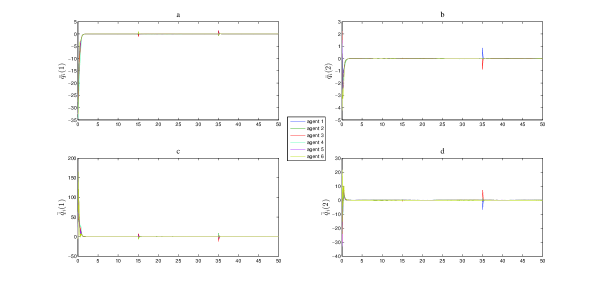
Figure 3: Trajectories of ${\bar{q}}_{i}$ and ${\bar{\dot{q}}}_{i}$ under $\mathcal{G}$.

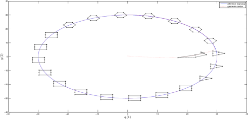
Figure 4: Trajectories and the formation of the six robots under $\mathcal{G}$.

The simulation results are presented in Fig.3 and Fig.4. Fig.3 shows that the tracking errors ${\bar{q}}_{i}$ and ${\bar{\dot{q}}}_{i}$ defined in (5) converge to zero in finite time at each dwell time interval, which means the time-varying formations of the MMS in the 2D plane and the tracking of the leader can be achieved simultaneously, $i.e.$, the time-varying formation tracking is accomplished. Additionally, the trajectory of the manipulators in 2D space is illustrated in Fig.4. It follows that the robots can reach the desired time-varying formation and the geometric center of the MMS follows the leader as required. It is clear in Fig.3 and Fig.4 that using the control algorithm (7) under the aforementioned configurations, the time-varying formation tracking can be achieved for the MMS.

Remark 7.

It is shown from picture $b$ and $d$ in Fig.3 that the second elements of ${\bar{q}}_{i}$ and ${\bar{\dot{q}}}_{i}$ do not change at the switching time instant $t=15$. Note that the time-varying formation $\digamma(t)$ changes from $\digamma_{0}$ to $\digamma_{1}$. By the set of $\digamma_{0}$ and $\digamma_{1}$ in Table 1, $b_{si}$ stays the same at the switching time instant $t=15$, which thus gives that ${\bar{q}}_{i}$ and ${\bar{\dot{q}}}_{i}$ do not change at the switching time instant.

5 Conclusion

For multiple manipulator systems (MMSs) under fixed and switching graphs, the time-varying formation tracking problem is addressed using inverse dynamics control technologies. Based on the functional characteristics of MMSs, an explicit formulation of time-varying formation is presented. The conditions (including sufficient conditions, necessary and sufficient conditions) on the interaction topology and control parameters are derived. Simulation results are presented to verify the effectiveness of the proposed algorithms. A few interesting issues, which are not addressed in this paper, concern the time-varying formation tracking problems of uncertain Euler-Lagrange systems and the extension of the presented approaches to the case of the polynomial trajectories. These issues will be considered in our future work.

References

• [1] Y. Wu, H. Su, P. Shi, Z. Shu, Z.G. Wu, Consensus of multiagent systems using aperiodic sampled-data control, IEEE Trans. Cybern. (2015) DOI: 10.1109/TCYB.2015.2466115.
• [2] H.X. Hu, W. Yu, Q. Xuan, L. Yu, G. Xie, Consensus of multi-agent systems in the cooperation-competition network with inherent nonlinear dynamics: A time-delayed control approach, Neurocomputing 158 (2015) 134-143.
• [3] W. Wang, G. Xie, Online high-precision probabilistic localization of robotic fish using visual and inertial cues, IEEE Trans. Ind. Electron. 62 (2) (2015) 1113-1124.
• [4] X.W. Jiang, Z.H. Guan, G. Feng, Y. Wu, F.S. Yuan, Optimal tracking performance of networked control systems with channel input power constraint, IET Control Theory Appl. 6 (11) (2012) 1690-1698.
• [5] Z.W. Liu, X. Yu, Z.H. Guan, C. Li, Pulse-modulated intermittent control in consensus of multi-agent systems, IEEE Trans. Syst., Man, Cybern. Syst. (2015) In Press.
• [6] R. Lu, W. Yu, J. LΓΌ, A. Xue, Synchronization on complex networks of networks, IEEE Trans. Neural Netw. Learn. Syst. 25 (11) (2014) 2110-2118.
• [7] R. Lu, W. Yu, J. LΓΌ, A. Xue, Synchronization on complex networks of networks, IEEE Trans. Neural Netw. Learn. Syst. DOI: 10.1109/TNNLS.2015.2503772.
• [8] G. Serpen, L. Liu. Parallel and distributed neurocomputing with wireless sensor networks. Neurocomputing (2015) DOI: 10.1016/j.neucom.2015.08.074.
• [9] B. Shen, Z. Wang, H. Dong, S. Zhang, Finite-horizon distributed $H\infty$ fault estimation for time-varying systems in sensor networks: a krein-space approach, IFAC-PapersOnLine 48 (21) (2015) 48-53.
• [10] H. Dong, Z. Wang, H. Gao, Distributed $H\infty$ filtering for a class of Markovian jump nonlinear time-delay systems over lossy sensor networks, IEEE Trans. Ind. Electron. 60 (10) (2013) 4665-4672.
• [11] S. Ueki, H. Kawasaki, T. Mouri, Adaptive coordinated control of multi-fingered robot hand, J. Robot. Mechatron. 21 (1) (2009) 36-43.
• [12] M.F. Ge, Z.H. Guan, T. Li, D.X. Zhang, R.Q. Liao, Robust mode-free sliding mode control of multi-fingered hand with position synchronization in the task space, Intelligent Robotics and Applications, Springer Berlin Heidelberg (2012) 571-580.
• [13] L. BriΓ±Γ³n-Arranz, A. Seuret, C. Canudas-de-Wit, Cooperative control design for time-varying formations of multi-agent systems, IEEE Trans. Autom. Control 59 (8) (2014) 2283-2288.
• [14] R.W. Beard, J. Lawton, F.Y. Hadaegh, A coordination architecture for spacecraft formation control, IEEE Trans. Control Syst. Technol. 9 (6) (2001) 777-790.
• [15] J.R.T. Lawton, R.W. Beard, B.J. Young, A decentralized approach to formation maneuvers, IEEE Trans. Robot. Autom. 19 (6) (2003) 933-941.
• [16] J.W. Kwon, D. Chwa, Hierarchical formation control based on a vector field method for wheeled mobile robots, IEEE Trans. Robot. 28 (6) (2012) 1335-1345.
• [17] A. Mahmood, Y. Kim, Leader-following formation control of quadcopters with heading synchronization, Aerosp. Sci. Technol. 47 (2015) 68-74.
• [18] X.N. Gao, L.J. Wu, Multi-robot formation control based on the artificial potential field method, Applied Mechanics and Materials, 519 (2014) 1360-1363.
• [19] X. Dong, B. Yu, Z. Shi, Y. Zhong, Time-varying formation control for unmanned aerial vehicles: theories and applications, IEEE Trans. Control Syst. Technol. 23 (1) (2015) 340-348.
• [20] R. Rahimi, F. Abdollahi, K. Naqshi, Time-varying formation control of a collaborative heterogeneous multi-agent system, Robot. Auton. Syst. 62 (2014) 1799-1805.
• [21] G. Antonelli, F. Arrichiello, F. Caccavale, A. Marino, Decentralized time-varying formation control for multi-robot systems, Int. J. Robot. Res. 33 (7) (2014) 1029-1043.
• [22] L. Cheng, Z.G. Hou, M. Tan, Decentralized adaptive consensus control for multi-manipulator system with uncertain dynamics, 2008 IEEE International Conference on Systems, Man and Cybernetics (SMC 2008) pp. 2712-2717.
• [23] L. Cheng, Z.G. Hou, M. Tan, Decentralized adaptive leader-follower control of multi-manipulator system with uncertain dynamics, 2008 IEEE International Conference on Industrial Electronics (IECON 2008) pp. 1608-1613.
• [24] J. Mei, W. Ren, G.F. Ma, Distributed containment control for lagrangian networks with parametric uncertainties under a directed graph, Automatica 48 (4) (2012) 653-659.
• [25] F. Chen, G. Feng, L. Liu, W. Ren, Distributed average tracking of networked Euler-lagrange systems, IEEE Trans. Autom. Control 60 (2) (2015) 547-552.
• [26] X. Liang, H. Wang, Y.H. Liu, W. Chen, G. Hu, Adaptive task-space cooperative tracking control of networked robotic manipulators without task-space velocity measurements, IEEE Trans. Cybern. (2015) DOI: 10.1109/TCYB.2015.2477606.
• [27] H.L. Wang, Passivity based synchronization for networked robotic systems with uncertain kinematics and dynamics, Automatica 49 (3) (2013) 755-761.
• [28] H.L. Wang, Task-space synchronization of networked robotic systems with uncertain kinematics and dynamics, IEEE Trans. Autom. Control, 58 (12) (2013) 3169-3174.
• [29] Y. Xu, W. Zhou, J. Fang, C. Xie, D. Tong, Finite-time synchronization of the complex dynamical network with non-derivative and derivative coupling, Neurocomputing (2015) DOI: 10.1016/j.neucom.2015.09.008.
• [30] G. Zong, R. Wang, W. Zheng, L. Hou, Finite-time H$\infty$ control for discrete-time switched nonlinear systems with time delay, Int. J. Robust Nonlinear Control 25 (6) (2015) 914-936.
• [31] J. Huang, C. Wen, W. Wang, Y.D. Song, Adaptive finite-time consensus control of a group of uncertain nonlinear mechanical systems, Automatica (51) (2015) 292-301.
• [32] Z.H. Guan, B. Hu, M. Chi, D.X. He, X.M. Cheng, Guaranteed performance consensus in second-order multi-agent systems with hybrid impulsive control, Automatica 50 (9) (2014) 2415-2418.
• [33] Z.W.Β Liu, Z.H.Β Guan, X.Β Shen, G.Β Feng, Consensus of multi-agent networks with aperiodic sampled communication via impulsive algorithms using position-only measurements, IEEE Trans. Autom. Control 57 (10) (2012) 2639-2643.
• [34] S.J. Yoo, T.H. Kim, Distributed formation tracking of networked mobile robots under unknown slippage effects, Automatica 54 (2015) 100-106.
• [35] F.L. Lewis, D.M. Dawson, C.T. Abdallah, Robot manipulator control: theory and practice. New York: Marcel Dekker, 2004.
• [36] Z. Meng, D.V. Dimarogonas, K.H. Johansson, Leader-follower coordinated tracking of multiple heterogeneous lagrange systems using continuous control, IEEE Trans. Robot. 30 (3) (2014) 739-745.
• [37] Y. Cao, W. Ren, Distributed coordinated tracking with reduced interaction via a variable structure approach, IEEE Trans. Autom. Control 57 (1) (2012) 33-48.
• [38] L. Cheng, Y. Wang, W. Ren, Z. G. Hou, M. Tan, Containment control of multiagent systems with dynamic leaders based on a $PI^{n}$-Type approach, IEEE Trans. Cybern. (2015) DOI: 10.1109/TCYB.2015.2494738.
• [39] Y. Wang, L. Cheng, Z.G. Hou, M. Tan, G. Bian, Polynomial trajectory tracking of networked Euler-Lagrange systems, in Proceedings of the 33rd Chinese Control Conference, July 28-30, 2014, Nanjing, China, pp. 1568-1573.
• [40] Y. Hong, Y. Xu, J. Huang, Finite-time control for robot manipulators, Syst. Contr. Lett. 46 (4) (2002) 243-253.
• [41] N. Rouche, P. Habets, M. Laloy, Stability Theory by Lyapunov s Direct Method. New York: Springer-Verlag, 1977.
• [42] L. Rosier, Homogeneous Lyapunov function for homogeneous continuous vector field, Syst. Contr. Lett. 9 (1992) 467-473.
• [43] M.W. Spong, R. Ortega, On adaptive inverse dynamics control of rigid robots, IEEE Trans. Autom. Control 35 (1) (1990) 92-95.
• [44] H. Wang, Y. Xie, Adaptive inverse dynamics control of robots with uncertain kinematics and dynamics, Automatica 45 (9) (2009) 2114-2119.
• [45] Y. Su, C. Zheng, Global finite-time inverse tracking control of robot manipulators, Robot. CIM-Int. Manuf. 27 (2011) 550-557.
• [46] X. Wang, Y. Hong, Distributed finite-time $\chi$-consensus algorithms for multi-agent systems with variable coupling topology, J. Syst. Sci. Complex 23 (2010) 209-218.