On the Resistance of Nearest Neighbor
To Random Noisy Labels
Abstract
Nearest neighbor has always been one of the most appealing non-parametric approaches in machine learning, pattern recognition, computer vision, etc. Previous empirical studies partly shows that nearest neighbor is resistant to noise, yet there is a lack of deep analysis. This work presents the finite-sample and distribution-dependent bounds on the consistency of nearest neighbor in the random noise setting. The theoretical results show that, for asymmetric noises, -nearest neighbor is robust enough to classify most data correctly, except for a handful of examples, whose labels are totally misled by random noises. For symmetric noises, however, -nearest neighbor achieves the same consistent rate as that of noise-free setting, which verifies the resistance of -nearest neighbor to random noisy labels. Motivated by the theoretical analysis, we propose the Robust -Nearest Neighbor (RNN) approach to deal with noisy labels. The basic idea is to make unilateral corrections to examples, whose labels are totally misled by random noises, and classify the others directly by utilizing the robustness of -nearest neighbor. We verify the effectiveness of the proposed algorithm both theoretically and empirically.
keywords:
Classification , nearest neighbor , random noise , consistency1 Introduction
The nearest neighbor (Cover and Hart,, 1967; Fix and Hodges,, 1951) has been one of the oldest and most intuitive approaches in pattern recognition, machine learning, computer vision, etc. The basic idea is to classify each unlabeled instance by the label of its nearest neighbor (-NN) or by the majority labels of nearest neighbors (-NN). Despite of simplicity, nearest neighbor takes good performance in real applications, and makes good explanations of predictions with theoretical guarantee (Berlind and Urner,, 2015; Biau and Devroye,, 2015; Dasgupta,, 2012; Kontorovich et al.,, 2017; Kontorovich and Weiss,, 2014; Kpotufe,, 2011; Kulkarni and Posner,, 1995; Shalev-Shwartz and Ben-David,, 2014; Wagner,, 1971). Empirical studies partially demonstrate the resistance of -nearest neighbor to noise (Kusner et al.,, 2014; Tarlow et al.,, 2013), whereas there is a paucity of deep understanding.
This work focuses on binary classification in the presence of random classification noises (Angluin and Laird,, 1988), that is, each observed label has been flipped with certain probability instead of seeing the ground-truth label, and training data of each class are contaminated by samples from the other class. Generally speaking, noisy data may disturb learning process, increase sample and model complexities, and deteriorate effectiveness and quality of learned classifiers. For example, the random noise defeats all convex potential boosters (Long and Servedio,, 2010), and support vector machines (SVMs) are sensitive to noisy labels. Many practical algorithms have been developed to tackle noisy labels (Angluin and Laird,, 1988; Kearns,, 1993; Lawrence and Schölkopf,, 2001; Liu and Tao,, 2016; Natarajan et al.,, 2013; Xu et al.,, 2006), most working with parametric classifiers, yet relatively few studies focus on non-parametric classifiers.
This work presents a theoretical and empirical understanding on the resistance of nearest neighbor to random noisy labels, and the main contributions can be summarized as follows:
-
1.
We provide the finite-sample and distribution-dependent bounds on the consistency of nearest neighbor. Our theoretical results show that, for asymmetric noises, -nearest neighbor is robust enough to classify most data correctly, except for a handful of totally misled examples. For symmetric noises, however, -nearest neighbor achieves the same consistent rate as that of noise-free setting, which verifies the resistance of -nearest neighbor. We also prove the inconsistency of -nearest neighbor even for symmetric noises.
-
2.
Motivated by the theoretical analysis, we propose the Robust -Nearest Neighbor (RNN) approach to deal with noisy labels with theoretical guarantee. The basic idea is to make unilateral corrections to examples whose labels are misled totally by random noise, and classify the others simultaneously by utilizing the robustness of -nearest neighbor. Our approach also makes use of nearest neighbor to estimate noise from corrupted datasets.
-
3.
Extensive experiments show the effectiveness of our RNN algorithm on benchmark datasets, and theoretical results are also verified empirically on synthetic dataset.
Related Work
The random noise model (Angluin and Laird,, 1988) has motivated a series of follow-up studies in the theoretical community. The finite VC-dimension has been used to characterize the learnability in (Aslam and Decatur,, 1996; Cesa-Bianchi et al.,, 1999), and Ben-David et al., (2009) showed the equivalence between Littlestone dimension and learnability of online mistake bound. Kearns, (1993) proposed the famous statistical query (SQ) model by capturing global statistical properties of large samples rather than individual example. Kalai and Servediob, (2005) made theoretical analysis of boosting algorithms in the presence of random noise.
Various practical approaches have been developed to deal with noisy data during the past decades, e.g., outlier detection (Barandela and Gasca,, 2000; Brodley and Friedl,, 1999), re-weights of training instances (Liu and Tao,, 2016; Rebbapragada and Brodley,, 2007; Wang et al., 2017a, ), perceptron-style algorithms (Bylander,, 1994; Crammer et al.,, 2006; Dredze et al.,, 2008), robust losses (Denchev et al.,, 2012; Masnadi-Shirazi and Vasconcelos,, 2009; Xu et al.,, 2006), unbiased losses (Gao et al.,, 2016; Natarajan et al.,, 2013), etc. The interested readers are also referred to the survey (Frenay and Verleysen,, 2014, reference therein).
Nearest neighbor has attracted much attention during the past decades (Beygelzimer et al.,, 2006; Cover and Hart,, 1967; Fix and Hodges,, 1951; Kontorovich et al.,, 2016; Kontorovich and Weiss,, 2015; Kulkarni and Posner,, 1995; Samworth,, 2012; Wagner,, 1971; Wang et al., 2017b, ). The asymptotic consistency of nearest neighbor has been studied in (Cover and Hart,, 1967; Dasgupta,, 2012; Devroye et al.,, 1994, 1996; Fix and Hodges,, 1951; Stone,, 1977). It is well-known that the classification error converges to Bayes error for -nearest neighbor when , and to for -nearest neighbor, and is at most for -nearest neighbor. The consistency analysis based on finite sample has also explored in the works of (Chaudhuri and Dasgupta,, 2014; Shalev-Shwartz and Ben-David,, 2014).
The rest of this paper is organized as follows. Section 2 presents some preliminaries. Section 3 provides theoretical analysis. Section 4 develops the Robust -Nearest Neighbor (RNN) approach. Section 5 presents detailed proofs for our main results. Section 6 conducts empirical studies. Section 7 concludes this work with future work.
2 Preliminaries
Let and denote the instance and label space, respectively. Suppose that is an (unknown) underlying distribution over the product space . Let be the marginal distribution over . Denote by conditional probability with respect to distribution . In this work, we assume that is -Lipschitz for some constant , that is,
Intuitively, this assumption implies that two instances are likely to have similar labels if they are close to each other, and such assumption has been taken in classification (Cover and Hart,, 1967; Shalev-Shwartz and Ben-David,, 2014). For a hypothesis , we define the classification error with respect to distribution as
Here, denotes the indicator function, which returns 1 if the argument is true and 0 otherwise. It is well-known (Devroye et al.,, 1996) that the Bayes classifier, which minimizes classification error, is given by , and the Bayes error is given by .
Let be a training data, where each example is drawn i.i.d. from distribution . In the random noise model, we can not observe the true labels (), and instead, each label has been flipped with a certain probability instead of seeing the true label, i.e., each label is corrupted by random noise with proportions and . Here
Throughout this work, we assume as in (Blum and Mitchell,, 1998). Let be the corrupted data, and denotes the corrupted distribution from true distribution by random noises with proportions and . Let be the corrupted conditional probability w.r.t. distribution . It is easy to get the relationship between and as follows:
| (1) |
We further have , and if is -Lipschitz, then is -Lipschitz, i.e.,
| (2) |
It is interesting to discuss the Tsybakov noise condition (Tsybakov,, 2004), i.e., for some finite and , we have
which presents faster convergence rate (Tsybakov,, 2004) in noise-free setting. It is noteworthy that this assumption is over true distribution , while the random noise setting does not make any assumption over . From Eqn. (1), we have the corrupted conditional probability such that
if the Tsybakov noise condition holds for distribution . This implies that Tsybakov noise condition can not be guaranteed for asymmetric noise even if the true distribution does. We consider the general random noise model without assumption over distribution in this work, and it is interesting to study random noise model for distribution with Tsybakov noise condition.
Let for integer . Denote by B a Bernoulli distribution of parameter , and represents that random variable is drawn from Bernoulli distribution B. We do not know the true data , noise proportions and , and distributions and in practice, and what we can observe is a corrupted data . The goal of this work is to learn a hypothesis with lower classification error over true distribution , but it is trained on the corrupted data .
3 Theoretical Analysis
Given corrupted training data and instance , let
be a reordering of according to their distances to , that is, . For -nearest neighbor algorithm, the output hypothesis is given by
Let denote the boundary set of Bayes’s classifier with respect to distribution , and we further introduce, for ,
where and show the most correctly predictive sets of positive and negative instances in the noise setting, respectively. Denote by
where the labels are relatively hard to be predicted correctly. It is important to introduce the set
| (3) |
where the labels are totally misled by random noise. We first present the consistency analysis of -nearest neighbour in the random noise setting.
Theorem 1
Let be a corrupted sample with noise proportions and . Let be the output hypothesis of applying -nearest neighbor to . We have
where .
Notice that the hypothesis of -nearest neighbor is trained on the corrupted sample , while denotes the classification error over the true distribution . The detailed proof is given in Section 5.1. Based on this theorem, we have
| (4) |
for and as .
As can be seen, the classification error of -nearest neighbor is biased at most from the Bayes error in the asymptotic convergence. Hence, -nearest neighbor is robust enough to classify most examples correctly, except for examples in , whose labels are totally misled. This motivates us to design effective strategy to tackle , which will be shown in Section 4.
For symmetric noises , we have from Eqn. (1), which proves the consistency of -nearest neighbor. Actually, we can further provide a stronger theorem, and the detailed proof is presented in Section 5.2.
Theorem 2
For and , we have
This theorem shows that
and we also have
Hence, the consistent rate of -nearest neighbors in the symmetric noise setting are the same as that of noise-free setting (Biau and Devroye,, 2015; Chaudhuri and Dasgupta,, 2014; Dasgupta,, 2012; Devroye,, 1981; Fix and Hodges,, 1951; Shalev-Shwartz and Ben-David,, 2014; Stone,, 1977), which proves the resistance of -nearest neighbor, particularly for large .
From Theorem 2, we present consistency analysis for -nearest neighbor in the noise-free setting:
Corollary 1
For and , we have
This corollary improves the work of (Shalev-Shwartz and Ben-David,, 2014, Theorem 19.5), which can be written (with our notations) as
As can be seen, the above shows the consistency of nearest neighbor as , while Corollary 1 presents tighter consistent rate of nearest neighbor as .
We finally study the inconsistency of -nearest neighbor even for symmetric noise as follows.
Theorem 3
Let be the output hypothesis of applying -nearest neighbor to . For , we have
4 The RNN Approach
Motivated from the preceding theoretical analysis, -nearest neighbor is robust enough to tackle most data except for examples in , whose labels are totally misled by random noises. Therefore, our basic idea is to develop effective strategies to classify examples in correctly, and classify the others simultaneously by utilizing the robustness of -nearest neighbor.
From Eqns. (1) and (3), we have
and
For , this follows that
because we have if and ; we also have if , which implies . In a similar manner, we have, for ,
This motivates us to make unilateral corrections to corrupted labels in . Specifically, we predict the label as for instance if and ; and predict as for instance if and .
The conditional probability is unknown in practice, and what we can observe is a training data . Let be nearest neighbors of instance , and we approximate , where is called predictive parameter.
We call such method Robust -Nearest Neighbor (RNN). Under the prior knowledge of noise proportions and , we can prove the consistency of RNN as follows.
Theorem 4
Let be a corrupted sample with noise proportions and . Let be the output hypothesis of applying our RNN approach to . For constant , we have
as ; we also have, for and as ,
As we can see, the RNN approach achieves the same consistent rate as that of traditional -nearest neighbor in the noise-free setting. Notice that the prior knowledge of and is also necessary for the proof of consistency of ERMs as in the work of (Natarajan et al.,, 2013). The detailed proof is presented in Section 5.4.
How to estimate noise proportions and from a corrupted sample has been an interesting and well-studied problem (Liu and Tao,, 2016; Menon et al.,, 2015; Ramaswamy et al.,, 2016; Scott et al.,, 2013). We follow the idea of conditional probability as in (Liu and Tao,, 2016; Menon et al.,, 2015), but introduce another -nearest neighbor rather than learning the corrupted conditional distribution.
Input: Corrupted sample , new instance , predictive parameter and noise parameter
Output: the predicted label
Specifically, let be the nearest neighbors of example . We approximate , where and is called noise parameter. As in the works of (Liu and Tao,, 2016; Menon et al.,, 2015), the estimated noise proportions and can be given, respectively, by
| (5) |
Algorithm 1 presents the detailed description of the proposed RNN method, and it can be further simplified to be traditional -nearest neighbor classification when .
5 Proofs
This section present the detailed proofs for our main results.
5.1 Proof of Theorem 1
The proof techniques are partially inspired by the works of (Chaudhuri and Dasgupta,, 2014; Shalev-Shwartz and Ben-David,, 2014). By the union bounds, we have
| (6) | |||||
Fixed , let be the cover of with boxes of length , and we have . Denote by two random events
Based on total probability theorem, we have
| (7) | |||||
According to Lemma 1, the first term in the above can be upper bounded by
| (8) |
For the second term, we fix and . Assume that are -nearest neighbors of . Let be conditional probabilities w.r.t. corrupted distribution , and set .
If , then we have
If , then we set , and have
| (9) |
from by Eqn. (2). We also have
For -nearest neighbor, it holds that
Combining with Eqn. (9) and Chernoff’s bounds, we have
This follows that
and it is noteworthy of for .
Similarly, we prove that, for ,
| (10) |
and it is noteworthy of for .
Combining with Eqns. (6)-(10), we have
where . From , we set
which completes the proof of Theorem 1 by simple calculations.\qed
Lemma 1
(Shalev-Shwartz and Ben-David,, 2014, Lemma 19.6) Denote by a collection of subsets over some domain . Let be a data of samples drawn i.i.d. according to distribution . Then, for every , we have .
5.2 Proofs of Theorem 2
Fixed , let be the cover of instance space using boxes of length , as the proof in Section 5.1. We have , and denote by the events
Based on the total probability theorem, we have
This follows that
| (11) | |||||
where the inequality holds from the following inequality, by Lemma 1,
To upper bound Eqn.(11), we first fix the training instances and instance , and assume that are the -nearest neighbors, i.e., for . Let be the conditional probability w.r.t. distribution , and let be the conditional probability w.r.t. the corrupted distribution . We set and . This follows
| (12) |
because for every . We also have
| (13) | |||||
This follows that, from Lemma 5 and Eqn. (12),
| (14) | |||||
where the last equality holds from Lemma 2. We further have
which implies, by combining with Eqns. (11), (13) and (14),
By setting , this follows that
From Lemma 3, we have
for and . This completes the proof of Theorem 2.\qed
Lemma 2
For and , let . We have
Lemma 3
For , we have
Proof: Let , and this follows that
Therefore, is a decreasing function, and for . This completes the proof as desired. \qed
Lemma 4
For and , we have
Proof: We first write
and the derivative is given by
Solving gives the optimal solution
It is easy to find that
| (15) |
because is continuous for . We further have
where
where we use the facts and . Therefore, we have
This lemma follows by combining with Eqn. (15). \qed
Based on Lemma 4, we have
Lemma 5
For , let , where are independent Bernoulli random variables with parameters , respectively, i.e., for . We set , , and let Bernoulli random variable . We have
Proof: We will present detailed proof for , and similar consideration could be proceeded for . For , we have
and
Based on the Chernoff’s bound, we have
For , we have
where the first equality holds from , and the last inequality holds from Lemma 4. We complete the proof from the fact . \qed
5.3 Proof of Theorem 3
From the definition , we first observe that is the probability of training sample and such that is different from . We have
where from corrupted distribution . Given any two instances and , we have
For noisy label , we have
which implies
This follows that
Therefore, we have
| (17) | |||||
For Eqn. (17), we have from , and
where the last inequality holds from . This follows
| (18) |
For Eqn. (17), we have
| (19) | |||||
where the last inequality holds from and the -Lipschitz assumption of . This remains to bound , and we proceed exactly as in (Shalev-Shwartz and Ben-David,, 2014). Fixed , and let be the cover of instance space using boxes of length , where . We have for and in the same box; otherwise, . This follows that
From the fact that
we have
which implies that, by setting and from Lemma 6,
From Eqn. (19), we have
By combining the above with Eqns. (17)-(18), we complete the proof.\qed
Lemma 6
For integer , we have
Proof: Let . We have
By setting , we have and . This completes the proof. \qed
5.4 Proof of Theorem 4
The proof is similar to that of Theorem 1 in Section 5.1, whereas the boundary of corrupted conditional probability changes from to . Recall , and it is necessary to introduce two sets as follows
for . We denote by
| (20) | |||||
We now present a general theorem for the consistency of the proposed RNN algorithm as follows:
Theorem 5
Let be a corrupted sample with noise proportions and . Let be the output hypothesis of applying our RNN algorithm to . We have
where , .
This theorem is similar to Theorem 1, whereas the boundary of corrupted conditional probability changes from to by random noise. Based on Theorem 5, we have
if and as ; we also have
for constant as . From Eqn. (20), we have
which implies . This completes the proof of Theorem 4.
Proof of Theorem 5 Without loss of generality, we assume . Based on the total probability theorem, we have
| (21) | |||||
Fixed , let be the cover of with boxes of length , and we have . Denote by two random events
By total probability theorem, we have
| (22) | |||||
From Lemma 1, the first term in the above can be upper bounded by
| (23) |
For the second term, we fix and . Assume that are -nearest neighbors of . Let be conditional probabilities w.r.t. corrupted distribution , and set .
If , then we have
If , then we set , and have
| (24) |
from by Eqn. (2). We also have
For our RNN algorithm, it holds that, for
and for
This implies that
Combining with Eqn. (24) and Chernoff’s bounds, we have
This follows that
| (25) |
and it is noteworthy of for .
Similarly, we prove that, for ,
| (26) |
and it is noteworthy of for .
6 Experiments
This section verifies theoretical results on synthetic dataset in Section 6.1, and shows the effectiveness of RNN on benchmark datasets in Section 6.2, followed by parameter analysis in Section 6.3.
6.1 Synthetic Dataset
We consider the instance space , which is similar to synthetic dataset in (Berlind and Urner,, 2015). Let be a uniform distribution over , and . We select and examples (i.i.d) for training and testing, respectively. Given noise proportions , the labels of training data are flipped accordingly and independently for times with different random seeds, and the average classification error is calculated on test data without noise corruptions.
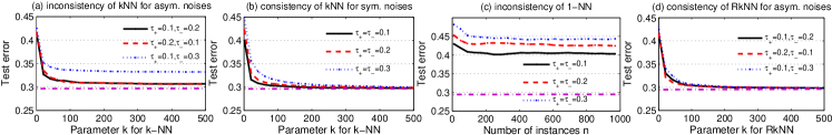
Figure 1(a) shows that, for asymmetric noises, test error of -nearest neighbor does not converge to Bayes error as increases, which is nicely in agreement with Theorem 1. Figure 1(b) shows the consistency of -nearest neighbor for symmetric noises and large , as expected in Theorem 2. Figure 1(c) shows the inconsistency of -nearest neighbor for symmetric noises as the sample size increases, which verifies Theorem 3 empirically. Figure 1(d) shows the consistency of our RNN approach for asymmetric noises, which presents good supports to Theorem 4.
6.2 Comparisons on Bechmark Datasets
We present empirical studies on twenty benchmark datasets111http://www.ics.uci.edu/~mlearn/MLRepository.html, and the details are summarized in Table 1. Most datasets have been used for learning with noisy labels, and the features have been scaled to for all datasets. Multi-class datasets have been transformed into binary ones by randomly partitioning classes into two groups, where each group contains the same cardinality of classes. We consider three groups of true noise proportions, that is, , and training labels are flipped accordingly with different random seeds.
We evaluate the performance of our RNN approach with traditional -nearest neighbor NN, as well as six state-of-the-art approaches on learning with noisy labels as follows.
-
1.
IR-KSVM: An importance-reweighting algorithm by kernel hinge-loss method (Liu and Tao,, 2016);
-
2.
IR-LLog: An importance-reweighting algorithm by linear logistic-loss method (Liu and Tao,, 2016)222The codes of IR-KSVM and IR-LLog are taken from http://tongliangliu.esy.es;
-
3.
LD-KSVM: A label-dependent algorithm by kernel hinge-loss method (Natarajan et al.,, 2013);
-
4.
UE-LLog: An unbiased-estimator algorithm by linear logistic-loss method (Natarajan et al.,, 2013);
-
5.
AROW: An adaptive regularization of weights (Crammer et al.,, 2009);
-
6.
NHERD: A normal (Gaussian) herd algorithm (Crammer and Lee,, 2010).
| datasets | #inst | #feat | datasets | #inst | #feat |
|---|---|---|---|---|---|
| heart | 270 | 13 | segment | 2,310 | 19 |
| ionosphere | 351 | 34 | landsat | 6,435 | 36 |
| housing | 506 | 13 | mushroom | 8,124 | 112 |
| cancer | 683 | 10 | usps | 9,298 | 256 |
| diabetes | 768 | 8 | pendigits | 10,992 | 16 |
| vehicle | 846 | 18 | letter | 15,000 | 16 |
| fourclass | 862 | 2 | magic04 | 19,020 | 10 |
| german | 1,000 | 24 | w8a | 49,749 | 300 |
| splice | 1,000 | 60 | shuttle | 58,000 | 9 |
| optdigits | 1,143 | 42 | acoustic | 78,823 | 50 |
For our RNN approach, four-fold cross validation is executed to select predictive parameter and noise parameter . For IR-KSVM and IR-LLog, we take the default parameters as in (Liu and Tao,, 2016). For LD-KSVM, we adopt the Gaussion kernels with best width trained by traditional SVM on noise-free data, as introduced in Natarajan et al., (2013). For UE-LLog, AROW and NHERD, four-fold cross validation is also executed for parameter selections.
| datasets | Our RNN | IR-KSVM | IR-LLog | LD-KSVM | UE-LLog | AROW | NHERD | NN | |
| heart | (0.1, 0.2) | .8544.0452 | .7941.0318 | .7088.1302 | .8000.0362 | .8029.0533 | .7721.0451 | .7721.0525 | .8353.0458 |
| (0.3, 0.1) | .8706.0403 | .8279.0505 | .6853.1395 | .8265.0474 | .8088.0500 | .7456.0654 | .7338.0954 | .8029.0267 | |
| (0.4, 0.4) | .7471.0706 | .5515.1299 | .6471.1226 | .6368.1304 | .6735.0917 | .6750.0691 | .6074.1397 | .7000.0305 | |
| ionosphere | (0.1, 0.2) | .8818.0229 | .8966.0281 | .8205.0363 | .8875.0323 | .8091.0374 | .8227.0409 | .7670.0611 | .8318.0450 |
| (0.3, 0.1) | .8705.0289 | .8795.0216 | .8284.0353 | .8841.0232 | .8045.0404 | .7818.0386 | .7341.1170 | .8545.0271 | |
| (0.4, 0.4) | .7705.0730 | .6727.1025 | .6989.1025 | .7341.1137 | .6727.0923 | .7102.0981 | .6227.1653 | .7932.0246 | |
| housing | (0.1, 0.2) | .8664.0181 | .8661.0246 | .8701.0145 | .8780.0179 | .8677.0257 | .8701.0201 | .8622.0197 | .8513.0223 |
| (0.3, 0.1) | .8693.0250 | .8583.0445 | .8693.0433 | .8677.0356 | .8654.0357 | .8751.0355 | .8614.0347 | .8409.0151 | |
| (0.4, 0.4) | .8157.0428 | .7756.0476 | .7874.0609 | .7173.0687 | .7976.0393 | .7787.0489 | .7063.1412 | .8085.0631 | |
| cancer | (0.1, 0.2) | .9731.0114 | .9673.0133 | .9661.0132 | .9690.0126 | .9567.0146 | .9696.0134 | .9690.0110 | .9754.0076 |
| (0.3, 0.1) | .9760.0125 | .9661.0120 | .9561.0181 | .9655.0164 | .9503.0223 | .9345.0308 | .9444.0362 | .9719.0151 | |
| (0.4, 0.4) | .9006.1031 | .9345.0324 | .8953.0370 | .8819.0642 | .8725.0670 | .9072.0425 | .8830.0499 | .9135.0877 | |
| diabetes | (0.1, 0.2) | .7531.0276 | .7641.0382 | .7464.0379 | .7651.0258 | .7578.0368 | .7603.0227 | .7500.0256 | .7354.0203 |
| (0.3, 0.1) | .7429.0361 | .7255.0430 | .7307.0449 | .7448.0358 | .7505.0332 | .7115.0342 | .7376.0434 | .7250.0419 | |
| (0.4, 0.4) | .6923.0659 | .6411.1044 | .6771.0641 | .6682.0905 | .6807.0874 | .6914.0769 | .7089.0403 | .6896.0709 | |
| vehicle | (0.1, 0.2) | .9615.0211 | .9624.0186 | .8725.1157 | .9615.0177 | .9330.0382 | .9459.0319 | .8734.1009 | .9450.0183 |
| (0.3, 0.1) | .9505.0230 | .9275.0285 | .6789.2000 | .9284.0255 | .9028.0426 | .9064.0538 | .8275.0915 | .9468.0364 | |
| (0.4, 0.4) | .8394.0514 | .7864.1495 | .6358.1104 | .7908.1154 | .7523.0852 | .8202.0729 | .7743.1212 | .8037.0724 | |
| fourclass | (0.1, 0.2) | .9968.0038 | .8130.0236 | .7528.0273 | .8074.0303 | .7583.0281 | .6926.0293 | .7204.0169 | .9907.0046 |
| (0.3, 0.1) | .9977.0024 | .8167.0304 | .7597.0282 | .8194.0298 | .7639.0261 | .6912.0259 | .7144.0461 | .9887.0065 | |
| (0.4, 0.4) | .8194.0556 | .7093.0580 | .6769.1031 | .7347.0755 | .7361.0468 | .7056.0285 | .7139.0317 | .8128.0589 | |
| german | (0.1, 0.2) | .7552.0197 | .6692.0259 | .7603.0259 | .6836.0299 | .7584.0267 | .6932.0302 | .6644.0234 | .7592.0290 |
| (0.3, 0.1) | .7460.0300 | .6932.0278 | .7340.0309 | .7056.0375 | .7388.0358 | .6784.0279 | .6424.0412 | .7040.0311 | |
| (0.4, 0.4) | .6704.0523 | .6100.0326 | .6696.0302 | .5752.0330 | .6648.0315 | .6128.0415 | .5824.0563 | .6944.0122 | |
| splice | (0.1, 0.2) | .7812.0357 | .7812.0273 | .7612.0388 | .8080.0318 | .7592.0221 | .6812.0248 | .6648.0230 | .7638.0276 |
| (0.3, 0.1) | .7720.0240 | .7384.0307 | .7524.0355 | .7764.0315 | .7448.0404 | .7000.0362 | .6840.0293 | .6488.0296 | |
| (0.4, 0.4) | .6708.0270 | .6180.0287 | .6428.0318 | .6180.0271 | .6288.0460 | .6012.0356 | .5740.0392 | .6587.0344 | |
| optdigits | (0.1, 0.2) | .9990.0017 | .9969.0020 | .9899.0058 | .9969.0026 | .9612.0121 | .9969.0020 | .9871.0168 | .9993.0016 |
| (0.3, 0.1) | .9958.0022 | .9948.0081 | .9720.0140 | .9969.0035 | .9483.0191 | .9657.0146 | .9476.0391 | .9916.0019 | |
| (0.4, 0.4) | .9745.0269 | .9587.0461 | .8084.1398 | .9682.0204 | .8517.0502 | .9269.0402 | .7892.1281 | .9685.0231 | |
| segment | (0.1, 0.2) | .8690.0109 | .8649.0136 | .7543.0150 | .8626.0160 | .7576.0171 | .7604.0178 | .7159.0555 | .8654.0093 |
| (0.3, 0.1) | .8663.0108 | .8600.0191 | .7356.0143 | .8561.0173 | .7526.0225 | .7543.0189 | .7104.0556 | .8526.0105 | |
| (0.4, 0.4) | .8123.0269 | .7469.0493 | .7057.0192 | .7804.0271 | .7067.0157 | .7145.0269 | .6249.0752 | .7941.0268 | |
| landsat | (0.1, 0.2) | .9213.0074 | .9183.0076 | .8656.0159 | .9208.0038 | .8711.0119 | .8485.0129 | .8210.0382 | .9231.0066 |
| (0.3, 0.1) | .9134.0070 | .9119.0139 | .8340.0159 | .9149.0059 | .8683.0078 | .8428.0099 | .7798.0569 | .9075.0105 | |
| (0.4, 0.4) | .8701.0132 | .6608.1223 | .7342.0633 | .8738.0099 | .7937.0243 | .8112.0137 | .6291.1047 | .8680.0091 | |
| mushroom | (0.1, 0.2) | .9985.0012 | .9975.0023 | .9980.0018 | .9983.0019 | .9900.0040 | .9975.0017 | .9923.0077 | .9987.0014 |
| (0.3, 0.1) | .9982.0013 | .9922.0079 | .9976.0029 | .9981.0015 | .9891.0072 | .9976.0018 | .9839.0192 | .9969.0021 | |
| (0.4, 0.4) | .9750.0093 | .9570.0280 | .9554.0261 | .9860.0086 | .9401.0090 | .9794.0081 | .7800.1429 | .9647.0099 | |
| usps | (0.1, 0.2) | .9680.0054 | .9775.0034 | .9007.0099 | .9782.0027 | .8993.0096 | .8889.0074 | .7896.0531 | .9720.0048 |
| (0.3, 0.1) | .9604.0038 | .9692.0053 | .8699.0108 | .9724.0039 | .8843.0080 | .8530.0137 | .6725.1158 | .9514.0052 | |
| (0.4, 0.4) | .8988.0160 | .7388.0227 | .7437.0342 | .9005.0124 | .7889.0298 | .8148.0149 | .6118.0634 | .9154.0123 | |
| pendigits | (0.1, 0.2) | .9927.0010 | .9965.0008 | .8360.0039 | .9974.0007 | .8398.0042 | .8371.0040 | .8081.0228 | .9926.0010 |
| (0.3, 0.1) | .9910.0023 | .9942.0014 | .8194.0083 | .9955.0013 | .8359.0049 | .8338.0057 | .8089.0207 | .9893.0021 | |
| (0.4, 0.4) | .9472.0127 | .8505.0416 | .6813.0518 | .9523.0092 | .8086.0123 | .8198.0053 | .6606.0586 | .9369.0156 | |
| letter | (0.1, 0.2) | .9290.0052 | .7805.0049 | .6754.0068 | .7647.0049 | .6748.0046 | .6723.0076 | .6686.0109 | .9284.0066 |
| (0.3, 0.1) | .9219.0058 | .7743.0066 | .6822.0080 | .7593.0055 | .6771.0075 | .6229.0108 | .6426.0152 | .9161.0054 | |
| (0.4, 0.4) | .7712.0099 | .6673.0438 | .5862.0547 | .7085.0142 | .6663.0100 | .6671.0096 | .6298.0345 | .7689.0071 | |
| magic04 | (0.1, 0.2) | .8315.0054 | .8136.0073 | .7904.0051 | .8171.0076 | .7921.0040 | .7935.0054 | .7909.0075 | .8291.0049 |
| (0.3, 0.1) | .8180.0044 | .8091.0030 | .7723.0045 | .8121.0035 | .7902.0039 | .7741.0045 | .7619.0199 | .8082.0023 | |
| (0.4, 0.4) | .7767.0089 | .7340.0118 | .7444.0186 | .7666.0239 | .7813.0109 | .7493.0104 | .7536.0290 | .7823.0078 | |
| w8a | (0.1, 0.2) | .9805.0015 | .9706.0015 | .9845.0006 | .9786.0015 | .9588.0135 | .8852.0030 | .8695.0132 | .9805.0014 |
| (0.3, 0.1) | .9807.0008 | .9708.0011 | .9825.0012 | .9781.0016 | .9614.0127 | .8897.0025 | .8829.0089 | .9803.0015 | |
| (0.4, 0.4) | .9769.0073 | .9696.0012 | .9774.0012 | .9720.0011 | .9152.0524 | .8377.0087 | .7451.0349 | .9528.0065 | |
| shuttle | (0.1, 0.2) | .9967.0006 | .9559.0060 | .9200.0117 | .9307.0035 | .8108.0042 | .8370.0060 | .8402.0140 | .9968.0008 |
| (0.3, 0.1) | .9958.0006 | .9335.0029 | .8339.0155 | .9252.0032 | .8099.0044 | .8290.0039 | .8385.0285 | .9952.0008 | |
| (0.4, 0.4) | .9550.0310 | .8415.0030 | .8056.0030 | .8451.0119 | .8005.0119 | .7987.0109 | .8273.0250 | .9696.0046 | |
| acoustic | (0.1, 0.2) | .7770.0012 | .7663.0033 | .7547.0039 | .7638.0036 | .7619.0033 | .7536.0028 | .7151.0629 | .7726.0016 |
| (0.3, 0.1) | .7700.0031 | .7629.0030 | .7477.0058 | .7609.0030 | .7620.0025 | .7141.0043 | .6553.0769 | .7579.0028 | |
| (0.4, 0.4) | .7575.0061 | .7396.0034 | .6079.0998 | .7445.0042 | .7560.0034 | .7532.0034 | .5470.0888 | .7111.0083 | |
| win/tie/loss | 35/20/5 | 45/15/0 | 28/25/7 | 47/13/0 | 49/11/0 | 53/7/0 | 23/33/4 | ||
Notice that we directly take the true noise proportions as priors in the implementations of the first four algorithms IR-KSVM, IR-LLog, LD-KSVM and UE-LLog. For RNN approach, however, we use -nearest neighbor to make estimations of noise proportions and from the corrupted training datasets. Obviously, it is an unfair comparison for RNN. The performances of the compared methods are evaluated by 10 trials of 4-fold cross validation with different random seeds, where the test accuracy is obtained by averaging over 40 runs, as summarized in Table 2.
It is evident that RNN is better than other four non-kernel algorithms IR-LLog, UE-LLog, AROW and NHERD. The win/tie/loss counts show that RNN is clearly superior to these non-kernel algorithms, as it wins for most times and never loses. It is also observable that RNN is highly competitive to two kernel methods IR-KSVM and LD-KSVM on most datasets, and RNN takes relatively stable performance while two kernel methods drop drastically as noise proportions increase. These observations validate the effectiveness of RNN, and the intuitive explanation is that RNN makes local corrections on a handful of totally misled examples, whereas the other methods on learning with noisy labels take global adjustments on loss functions, which may be sensitive to random noise. In comparisons with traditional NN, our RNN achieves better performance for asymmetric noises, and takes comparable performance for symmetric noise as expected.
Besides the frequent pairwise t-test shown in Table 2, we also consider Bayesian t-test (Wang and Liu,, 2016) to compare the performance of various algorithms, because our derivations of main results are based on a Bayesian framework. According to Bayesian t-test, the counts of win/tie/loss of our RkNN and compared methods are shown in Table 3. As we can see, Bayesian t-test takes better statistical support than frequent pairwise t-test to verify our proposed RkNN algorithm.
| our RkNN | IR-KSVM | IR-LLog | LD-KSVM | UE-LLog | AROW | NHERD | kNN |
| win/tie/loss | 39/16/5 | 46/12/2 | 32/20/8 | 48/12/0 | 51/8/1 | 53/7/0 | 30/25/5 |
| heart | ionosphere | housing | cancer | diabetes | |
| (0.1, 0.2) | (.050, .143) | (.009, .251) | (.036, .081) | (.013, .091) | (.003, .201) |
| (0.3, 0.1) | (.258, .039) | (.154, .115) | (.173, .003) | (.132, .000) | (.142, .098) |
| (0.4, 0.4) | (.232, .257) | (.177, .282) | (.200, .198) | (.184, .183) | (.181, .211) |
| vehicle | fourclass | german | splice | optdigits | |
| (0.1, 0.2) | (.005, .053) | (.004, .028) | (.123, .151) | (.107, .157) | (.000, .007) |
| (0.3, 0.1) | (.126, .020) | (.152, .000) | (.363, .015) | (.292, .025) | (.146, .000) |
| (0.4, 0.4) | (.196, .225) | (.195, .185) | (.243, .191) | (.215, .180) | (.160, .188) |
| segment | landsat | mushroom | usps | pendigits | |
| (0.1, 0.2) | (.001, .020) | (.000, .014) | (.000, .008) | (.000, .011) | (.000, .015) |
| (0.3, 0.1) | (.093, .000) | (.082, .000) | (.071, .000) | (.083, .000) | (.095, .000) |
| (0.4, 0.4) | (.168, .134) | (.108, .093) | (.112, .104) | (.117, .112) | (.084, .084) |
| letter | magic04 | w8a | shuttle | acoustic | |
| (0.1, 0.2) | (.000, .008) | (.001, .009) | (.060, .105) | (.001, .017) | (.000, .055) |
| (0.3, 0.1) | (.104, .000) | (.093, .002) | (.220, .000) | (.195, .001) | (.128, .000) |
| (0.4, 0.4) | (.093, .087) | (.081, .070) | (.275, .251) | (.094, .113) | (.135, .130) |
Table 4 shows the average noise proportions estimated by RNN on benchmark datasets. As we can see, the trend of true difference can be observed from the estimated difference in some way, though RNN seldom makes precise estimation on noise proportions and , particularly for large datasets and small noise proportions. It is also noticed that the RNN approach achieves good performance, as shown in Table 2, even for rather rough estimation on noise proportions. Those observations further validate the robustness of the RNN approach.
6.3 Parameter Influence
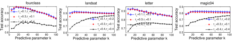
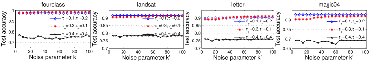
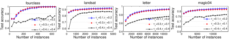
We investigate the influence of parameters in this section. Figure 4 shows that RNN is not sensitive to the values of predictive parameter given that it is not set smaller than 10, and we’d better take large when tackle large datasets and high noise proportions. Figure 4 shows that the noise parameter should not be set to value smaller than 20, and there is a relative big range between 20 and 100 where RNN achieves better performance. Figure 4 shows the convergence of performance as sample size increases, which illustrates that RNN takes stable and convergent performance as expected. Relevant analysis also shows the robustness of RNN. Here, we present empirical analysis of parameters on four datasets, while the trends are similar on other datasets.
7 Conclusion
This work presents the finite-sample and distribution-dependent bounds on the consistency of nearest neighbor. The theoretical results show that, for asymmetric noises, -nearest neighbor is robust enough to classify most data correctly, except for a handful of examples, whose labels are totally misled by random noises. For symmetric noises, however, -nearest neighbor achieves the same consistent rate as that of noise-free setting, which verifies the resistance of -nearest neighbor. Motivated from theoretical analysis, we propose the Robust -Nearest Neighbor (RNN) approach to deal with noisy labels. The basic idea is to make unilateral corrections to examples, whose labels are totally misled by random noises, and classify the others directly by utilizing the robustness of -nearest neighbor. Extensive experiments validate the effectiveness of the proposed RNN method. An interesting future work is to develop robust -nearest neighbor for large-scale and high-dimensional datasets in the random noise setting.
References
- Angluin and Laird, (1988) Angluin, D. and Laird, P. (1988). Learning from noisy examples. Machine Learning, 4(2):343–370.
- Aslam and Decatur, (1996) Aslam, J. and Decatur, S. (1996). On the sample complexity of noise-tolerant learning. Information Processing Letters, 57(4):189–195.
- Barandela and Gasca, (2000) Barandela, R. and Gasca, E. (2000). Decontamination of training samples for supervised pattern recognition methods. In Joint IAPR International Workshops on Statistical Techniques in Pattern Recognition and Structural and Syntactic Pattern Recognition, pages 621–630, Alicante, Spain.
- Ben-David et al., (2009) Ben-David, S., Pál, D., and Shalev-Shwartz, S. (2009). Agnostic online learning. In Proceedings of the 22nd Conference on Learning Theory, Montreal, Canada.
- Berlind and Urner, (2015) Berlind, C. and Urner, R. (2015). Active nearest neighbors in changing environments. In Proceeding of the the 32nd International Conference on Machine Learning, pages 1870–1879, Lille, France.
- Beygelzimer et al., (2006) Beygelzimer, A., Kakade, S., and Langford, J. (2006). Cover trees for nearest neighbor. In Proceedings of the 23rd International Conference on Machine Learning, pages 97–104, New York, NY.
- Biau and Devroye, (2015) Biau, G. and Devroye, L. (2015). Lectures on the Nearest Neighbor Method. Springer, New York.
- Blum and Mitchell, (1998) Blum, A. and Mitchell, T. (1998). Combining labeled and unlabeled data with co-training. In Proceedings of the 11st Annual Conference on Computational Learning Theory, pages 92–100, Madison, WI.
- Brodley and Friedl, (1999) Brodley, C. and Friedl, M. (1999). Identifying mislabeled training data. Journal of Artificial Intelligence Research, 11:131–167.
- Bylander, (1994) Bylander, T. (1994). Learning linear threshold functions in the presence of classification noise. In Proceeding of the 7th Conference on Learning Theory, New York, NY.
- Cesa-Bianchi et al., (1999) Cesa-Bianchi, N., Dichterman, E., Fischer, P., Shamir, E., and Simon, H. (1999). Sample-efficient strategies for learning in the presence of noise. Journal of the ACM, 46(5):684–719.
- Chaudhuri and Dasgupta, (2014) Chaudhuri, K. and Dasgupta, S. (2014). Rates of convergence for nearest neighbor classification. In Ghahramani, Z., Welling, M., Cortes, C., Lawrence, N., and Weinberger, K., editors, Advances in Neural Information Processing Systems 27, pages 3437–3445. MIT Press, Cambridge, MA.
- Cover and Hart, (1967) Cover, T. and Hart, P. (1967). Nearest neighbor pattern classification. IEEE Transactions on Information Theory, 13(1):21–27.
- Crammer et al., (2006) Crammer, K., Dekel, O., Keshet, J., Shalev-Shwartz, S., and Singer, Y. (2006). Online passive-aggressive algorithms. Journal of Machine Learning Research, 7:551–585.
- Crammer et al., (2009) Crammer, K., Kulesza, A., and Dredze, M. (2009). Adaptive regularization of weight vectors. In Advances in Neural Information Processing Systems 22, pages 414–42. MIT Press, Cambridge, MA.
- Crammer and Lee, (2010) Crammer, K. and Lee, D. (2010). Learning via gaussian herding. In Advances in Neural Information Processing Systems 23, pages 451–459. MIT Press, Cambridge, MA.
- Dasgupta, (2012) Dasgupta, S. (2012). Consistency of nearest neighbor classification under selective sampling. In Proceedings of the 25th Annual Conference on Learning Theory, pages 18.1–18.15, Edinburgh, Scotland.
- Denchev et al., (2012) Denchev, V., Ding, N., Neven, H., and Vishwanathan, S. (2012). Robust classification with adiabatic quantum optimization. In Proceedings of the 29th International Conference on Machine Learning, pages 863–870, Edinburgh, Scotland.
- Devroye, (1981) Devroye, L. (1981). On the inequality of cover and hart in nearest neighbor discrimination. IEEE Transactions on Pattern Analysis and Machine Intelligence, 3(1):75–78.
- Devroye et al., (1994) Devroye, L., Gyorfi, L., Krzyzak, A., and Lugosi, G. (1994). On the strong universal consistency of nearest neighbor regression function estimates. Annals of Statistics, 22:1371–1385.
- Devroye et al., (1996) Devroye, L., Györfi, L., and Lugosi, G. (1996). A Probabilistic Theory of Pattern Recognition. Springer, New York.
- Dredze et al., (2008) Dredze, M., Crammer, K., and Pereira, F. (2008). Confidence-weighted linear classification. In Proceedings of the 25th International Conference on Machine Learning, pages 264–271, Helsinki, Finland.
- Fix and Hodges, (1951) Fix, E. and Hodges, J. (1951). Discriminatory analysis, nonparametric discrimination. USAF School of Aviation Medicine, Randolph Field, Texas. Project 21-49-004, Report 4, Contract AD41(128)-31.
- Frenay and Verleysen, (2014) Frenay, B. and Verleysen, M. (2014). Classification in the presence of label noise: a survey. IEEE Transactions on Neural Networks and Learning System, 25(5):845–869.
- Gao et al., (2016) Gao, W., Wang, L., Li, Y.-F., and Zhou, Z.-H. (2016). Risk minimization in the presence of label noise. In Proceedings of the 30 AAAI Conference on Artificial Intelligence, pages 1575–1581, Phoenix, Arizona.
- Kalai and Servediob, (2005) Kalai, A. and Servediob, R. (2005). Boosting in the presence of noise. Journal of Computer and System Sciences, 71:266–290.
- Kearns, (1993) Kearns, M. (1993). Efficient noise-tolerant learning from statistical queries. In Proceedings of the 25th Annual ACM Symposium on Theory of Computing, pages 392–401, San Diego, CA.
- Kontorovich et al., (2016) Kontorovich, A., Sabato, S., and Urner, R. (2016). Active nearest-neighbor learning in metric spaces. In Advances in Neural Information Processing Systems 29, pages 856–864. MIT Press, Cambridge, MA.
- Kontorovich et al., (2017) Kontorovich, A., Sabato, S., and Weiss, R. (2017). Nearest-neighbor sample compression: Efficiency, consistency, infinite dimensions. In Advances in Neural Information Processing Systems 30, pages 1572–1582. MIT Press, Cambridge, MA.
- Kontorovich and Weiss, (2014) Kontorovich, A. and Weiss, R. (2014). Maximum margin multiclass nearest neighbors. In Proceedings of the 31st International Conference on Machine Learning, pages 892–900, Beijing, Chian.
- Kontorovich and Weiss, (2015) Kontorovich, A. and Weiss, R. (2015). A bayes consistent 1-nn classifier. In Proceedings of the 18th International Conference on Artificial Intelligence and Statistics, pages 480–488, Las Vegas, NV.
- Kpotufe, (2011) Kpotufe, S. (2011). -nn regression adapts to local intrinsic dimension. In Shawe-Taylor, J., Zemel, R., Bartlett, P., Pereira, F., and Weinberger, K., editors, Advances in Neural Information Processing Systems 19, pages 729–737. MIT Press, Cambridge, MA.
- Kulkarni and Posner, (1995) Kulkarni, S. and Posner, S. (1995). Rates of convergence of nearest neighbor estimation under arbitrary sampling. IEEE Transactions on Information Theory, 41(4):1028–1039.
- Kusner et al., (2014) Kusner, M., Tyree, S., Weinberger, K., and Agrawal, K. (2014). Stochastic neighbor compression. In Proceedings of the 31st International Conference on Machine Learning, pages 622–630, Beijing, China.
- Lawrence and Schölkopf, (2001) Lawrence, N. and Schölkopf, B. (2001). Estimating a kernel fisher discriminant in the presence of label noise. In Proceedings of the 8th International Conference on Machine Learning, pages 306–313, Williamstown, MA.
- Liu and Tao, (2016) Liu, T. and Tao, D. (2016). Classification with noisy labels by importance reweighting. IEEE Transactions on Pattern Analysis and Machine Intelligence, 38(3):447–461.
- Long and Servedio, (2010) Long, P. and Servedio, R. (2010). Random classification noise defeats all convex potential boosters. Machine Learning, 78(3):287–304.
- Masnadi-Shirazi and Vasconcelos, (2009) Masnadi-Shirazi, H. and Vasconcelos, N. (2009). On the design of loss functions for classification: Theory, robustness to outliers, and savageboost. In Advances in Neural Information Processing Systems 22, pages 1049–1056. MIT Press, Cambridge, MA.
- Menon et al., (2015) Menon, A., Rooyen, B., Ong, C., and Williamson, B. (2015). Learning from corrupted binary labels via class-probability estimation. In Proceedings of the 32nd International Conference on Machine Learning, pages 125–134, Lille, France.
- Natarajan et al., (2013) Natarajan, N., Dhillon, I., Ravikumar, P., and Tewari, A. (2013). Learning with noisy labels. In Advances in Neural Information Processing Systems 26, pages 1196–1204. MIT Press, Cambridge, MA.
- Ramaswamy et al., (2016) Ramaswamy, H., Scott, C., and Tewari, A. (2016). Mixture proportion estimation via kernel embeddings of distributions. In Proceedings of the 33rd International Conference on Machine Learning, pages 2052–2060, New York, NY.
- Rebbapragada and Brodley, (2007) Rebbapragada, U. and Brodley, C. (2007). Class noise mitigation through instance weighting. In Proceedings of the 18th European Conference on Machine Learning, pages 708–715, Warsaw, Poland.
- Samworth, (2012) Samworth, R. (2012). Optimal weighted nearest neighbour classifiers. Annals of Statistics, 40(5):2733–2763.
- Scott et al., (2013) Scott, C., Blanchard, G., and Handy, G. (2013). Classification with asymmetric label noise: Consistency and maximal denoising. In Proceedings of the 26th Annual Conference on Computational Learning Theory, pages 489–511.
- Shalev-Shwartz and Ben-David, (2014) Shalev-Shwartz, S. and Ben-David, S. (2014). Understanding Machine Learning: From Theory to Algorithms. Cambridge University Press, Cambridge.
- Stone, (1977) Stone, C. (1977). Consistent nonparametric regression. Annals of Statistics, 5:595–645.
- Tarlow et al., (2013) Tarlow, D., Swersky, K., Swersky, K., Charlin, L., Sutskever, I., and Zemel, R. (2013). Stochastic -neighborhood selection for supervised and unsupervised learning. In Proceedings of the 30th International Conference on Machine Learning, pages 199–207, Atlanta, GA.
- Tsybakov, (2004) Tsybakov, A. (2004). Optimal aggregation of classifiers in statistical learning. Annals of Statistics, 32(1):135–166.
- Wagner, (1971) Wagner, T. (1971). Convergence of the nearest neighbor rule. IEEE Transactions on Information Theory, 17(5):566–571.
- Wang and Liu, (2016) Wang, M. and Liu, G. (2016). A simple two-sample Bayesian t-test for hypothesis testing. American Statistician, 70(2):195–201.
- (51) Wang, R., Liu, T., and Tao, D. (2017a). Multiclass learning with partially corrupted labels. IEEE Transactions on Neural Networks and Learning Systems, 99:1–13.
- (52) Wang, Y., Jha, S., and Chaudhuri, K. (2017b). Analyzing the robustness of nearest neighbors to adversarial examples. CoRR/abstract, 1706.03922.
- Xu et al., (2006) Xu, L., Crammer, K., and Schuurmans, D. (2006). Robust support vector machine training via convex outlier ablation. In Proceedings of the 21st Conference on Artificial Intelligence, pages 536–542, Boston, MA.