Versõ foliõ: Diversified Ranking for Large Graphs with Context-Aware Considerations
Abstract
This work is pertaining to the diversified ranking of web-resources and interconnected documents that rely on a network-like structure, e.g. web-pages. A practical example of this would be a query for the most relevant web-pages that are also in the same time as dissimilar with each other as possible. Relevance and dissimilarity are quantified using an aggregation of network distance and context similarity. For example, for a specific configuration of the problem, we might be interested in web-pages that are similar with the query in terms of their textual description but distant from each other in terms of the web-graph, e.g. many clicks away. In retrospect, a dearth of work can be found in the literature addressing this problem taking the network structure formed by the document links into consideration. In addition, the vast majority of the approaches that have been proposed in the literature leverage greedy heuristics relying on certain measures that capture only some aspect of the problem. Arguably, this is not enough.
In this work, we propose a hill-climbing approach that is seeded with a document collection which is generated using greedy heuristics to diversify initially. More importantly, we tackle the problem in the context of web-pages where there is an underlying network structure connecting the available documents and resources. This is a significant difference to the majority of works that tackle the problem in terms of either content definitions, or the graph structure of the data, but never addressing both aspects simultaneously. To the best of our knowledge, this is the very first effort that can be found to combine both aspects of this important problem in an elegant fashion by also allowing a great degree of flexibility on how to configure the trade-offs of (i) document relevance over result-items’ dissimilarity, and (ii) network distance over content relevance or dissimilarity. Last but not least, we present an extensive evaluation of our methods that demonstrate the effectiveness and efficiency thereof.
category:
H.3.3 Information Search and Retrieval Search Process1 Introduction
Result diversification has lavished great scientific interest in recent years for it addresses a variety of problems simultaneously. First, modern information retrieval research focuses on result diversification as a means of counteracting intrinsic IR problems, like the over-specialization problem of retrieving too homogeneous results. For instance, for information queries, users reading through a list of relevant but redundant pages quickly stop as they do not expect to learn more. Therefore, new search techniques had to be improvised in order to ameliorate user satisfaction and decrease query abandonment. Second, diversification reduces the risk that none of the returned results satisfies a user’s query intent. For example query term “Apache” could pertain to the well-known software foundation, or the Native American tribe just as well. Similarly, among the results for “Python” we could find information about a reptile specie, a programming language, or even the Monty Python, a comedy group. Therefore, by focusing on just one genre of information, we could easily fail to answer the query properly, or even danger to be completely irrelevant. Also, among the most frequent examples found in the literature for ambiguous and exploratory queries “flash” and “jaguar” are the most typical for they can represent completely different things, e.g. cars, felines, etc. Ambiguity is a common and usual problem, a solution to which can be result diversification. Third, enabling diversity tacitly facilitates (near) duplicates elimination.
Besides, conventional information retrieval models presume that given a similarity measure with different degrees of relevancy, the relevance of a document is independent of the relevance of other documents. In reality however, this independence relevance assumption rarely holds; the utility of retrieving one document may depend on which documents the user has already seen. Regarding this complementary aspect of diversification, it is in general insufficient to simply return a set of relevant results, since correlations among them are also important. More specifically, documents should be selected progressively according to their relevance and also in terms with the documents that come before it. For example, a system that delivers documents that are relevant and novel must be able to identify relevant documents that are dissimilar to the previously delivered documents, in the sense of comprising new information. The main challenge in diversification lies in that these two important goals are contradictory to each other.

In essence, the goal of diversification is to identify a list of items that are dissimilar with each other, but nonetheless relevant to the user’s search criteria. In other words, the diversity is defined by how much each item of the result-set differs from the others in terms of their attribute values. In effect, diversification is a multifaceted problem with many practical and theoretical extensions. A profound and rich link with combinatorics and approximation is exploited in research works where diversification is performed through heuristics and greedy algorithms mostly. This work focuses on diversified ranking of web-resources and documents that rely on a network-like structure, e.g. web-pages. A typical example of this problem would be a query for the most relevant web-pages that are also in the same time as dissimilar with each other as possible. This is an important problem with deep rooted theoretical extensions and even more practical applications. It is a NP-hard problem and the fact that we address it in the context of data representing interconnected information, adds not only to the complexity of the problem, but also to the value of an effective and efficient solution that is capable of returning a near-optimal solution within a few seconds.
More specifically, there are two approaches proposed in this paper used in combination, one after the other, in an effort to maximize their effect. The first relies on greedy heuristics, whereas the second leverages a hill-climbing approach. According to the former, we compute diversified sets starting from the object in the network that is most similar to the query, given a metric that smooths network distance with context similarity, and we incrementally append to the set the object which when added to the result constructed so far, the rank of the outcome is better than it would be if we had added any other object. This process is repeated as many times as the desired number of elements. On the other hand, the latter approach, takes as input the greedily built diversified sets, and iteratively refines them by removing certain elements and replacing them with more preferable choices in order to produce better diversified sets. Each time we keep only the best derived sets we have retrieved so far, and we work on that collection of sets as a means to explore the overall search space.
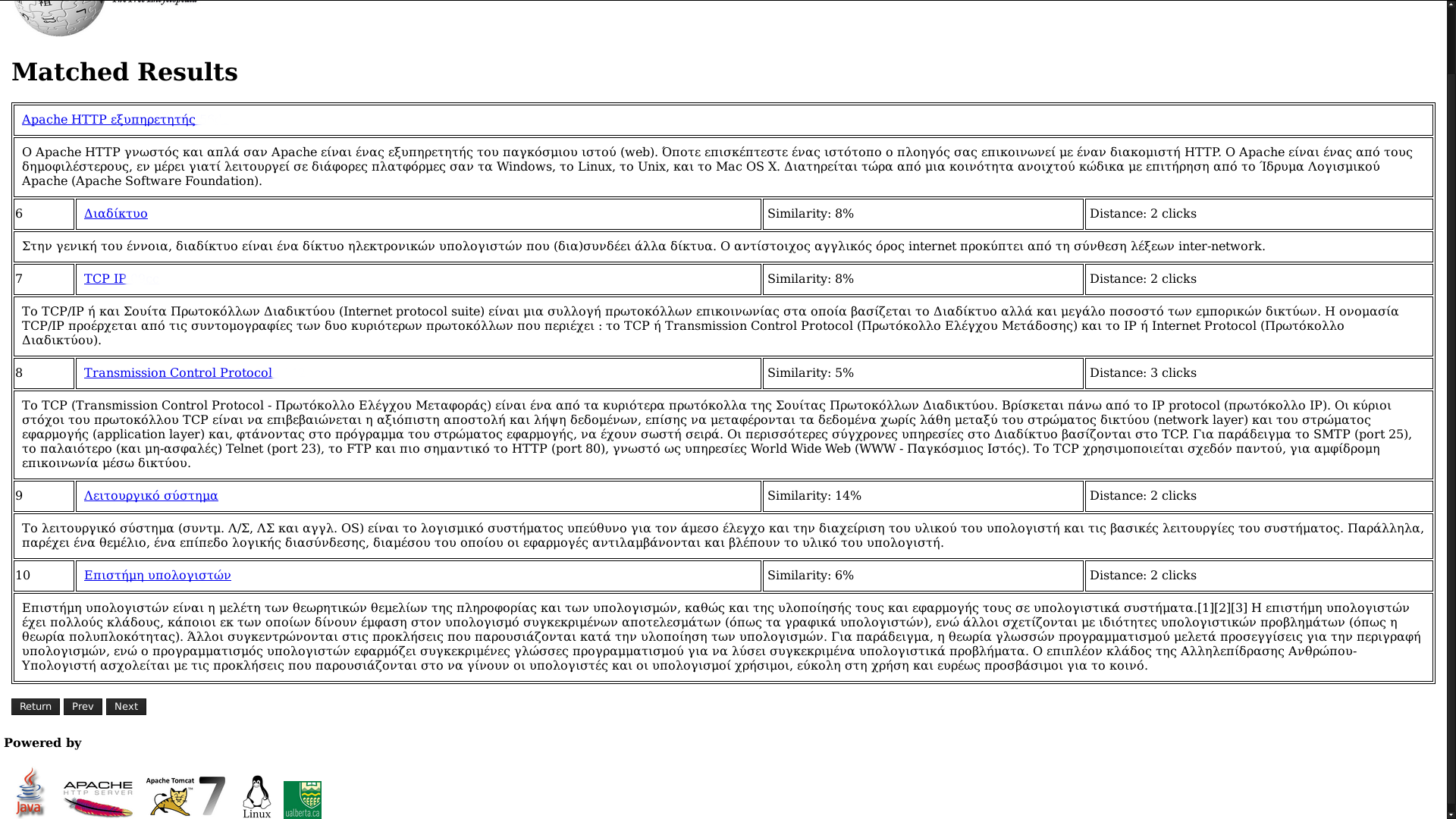
What is more, we prove our concept through a prototype that we launched on-line. It operates over multi-lingual collections of the Wikipedia dataset but other collections of web-pages can also be used as soon as the appropriate models are extracted, e.g. web-graph, a vector space model (based on tf-idfs in our case), etc. In Figure 1, we depict the results for “Apache”. Among those one can find links to articles up to 4 clicks away while still being relevant to the “Apache HTTP server”, the article which was chosen to serve as the query center for our search because of its title for it matches the query better than other articles. Among the top results “Server” and “Unix” are the closest articles that are also very similar to the query center in the same time. Of course, other close neighbors could have been selected, but we put special emphasis on the fact that those are quite diverse with each other as they belong to different categories, tacitly addressed though a model that relies on content-based definitions. When we examine the remaining results (not directly connected to the query center) we see links to other articles like “Computer Networks”, “Information Systems”, “Internet”, “Operating Systems”, and “Computer Science”, each contributing to the result by representing a different field or thematic area, tackling this way directly the over-specialization problem, the main challenge addressed in this paper. Other notions, like the page-rank of each web-page could easily be incorporated in our rank functions as a way to promote more important pages, exactly like we do with the relevant ones. All different criteria are smoothed according to the user preferances via an elegant interface.
In summary, the contributions of this paper are the following:
-
1.
We present verso, an algorithm which given a query object , a set of interconnected objects , and a ranking function , it retrieves the optimal single object, which when added in it is better ranked in terms of both network characteristics and textual descriptions of its elements, than it would be if any other point had been inserted.
-
2.
We propose a paradigm that combines a method based upon greedy heuristics with an approach leveraging a hill-climbing methodology to exploit verso, so as to construct diversified sets of arbitrary cardinality.
-
3.
We show through an extensive experimental evaluation that our paradigm clearly outperforms the BestCoverage method proposed in [12] in terms of response times, result quality, and memory requirements, as well.
-
4.
We developed in Java and made available on-line a prototype implementing our method.
As a final note, the name of our paradigm “versõ foliõ” translates from Latin to English as “the turned side of the page”. The remainder of this paper is organized as follows: Section 2 discusses contemporary diversification techniques over different types of data. A formal definition of the problem we study here is presented in Section 3. Our paradigm is presented in Section 4. Section 5 presents an extensive evaluation of our scheme. Finally, we conclude and summarize our contributions in Section 6.
2 Related Work
In this section, we present an overview of the literature on result diversification over two different fields.
2.1 Result Diversification for Structured Data
The first part of this section describes the various definitions of the result diversification problem proposed in the research literature and classifies the algorithms proposed for locating diverse items. A complete survey on the state of the art can be found in [5].
In the absence of any explicit knowledge of user intent, three main approaches are employed for result diversification: (i) content based, for differentiated result items in terms of their attribute values, (ii) novelty based, when promoting items that contain new information compared to those ranked higher, and (iii) coverage, for including items so as to cover as many categories as possible.
First and foremost, content-based definitions aim at maximizing the aggregated distance between any pair of objects in the result-set. Arguably, the most influential work on diversification is that of Maximal Marginal Relevance (MMR) [3]. In their seminal work, the authors introduced a trade-off between diversity and the relevance of search results through the combination of two similarity functions shown in Equation 1. One for measuring the similarity among a document collection , and the other the similarity between query and each document. In addition, parameter controls the degree of trade-off.
| (1) |
Moreover, [9] is another conspicuous work that follows an axiomatic approach to develop a set of natural axioms that a diversification system is expected to follow. A variety of methods are discussed, such as semantic distance-based schemes, taxonomy-based categorical distance schemes, and the advantages and disadvantages thereof. On the other hand, [21] focuses on diversification over structured data to propose an appropriate ranking-similarity function for a given ordering of the data attributes. An interesting approach is presented in [10] that extends the nearest neighbors problem with providing a minimum distance threshold among the points of the result-set in order to guarantee diversity. In a more recent work [8], the authors adopt an approach based on Voronoi cells in order to retrieve the object maximizing a novelty function. More specifically, items that already constitute the answer are appointed as cell centers. Then, all objects that happen to be placed on the vertices and the edges of the formed Voronoi diagram are examined and the best of them is inserted into the answer-set. Another similar approach is proposed in [22] which however requires knowing in advance all the objects to compute the objective function.
Novelty can be seen as a means to avoid redundancy and (near) duplicates, and also as a means to impart additional information to the result-set; whereas diversity is viewed as the need to resolve ambiguity. Adhering to this principle, queries and objects are treated as sets of “information nuggets” in [4], while relevance is a function of the nuggets contained in possible interpretations of the query and the result-set. In another line of work, [27] empowers adaptive filtering systems to distinguish novel and redundant items. Such systems identify items that are similar to previously delivered ones in having the same topic, but also dissimilar to them, in the sense of containing novel information.
Conversely, [23] suggests from the user point of view that “novelty seeking” is not equivalent to “diversity seeking”, and that the novelty preferences of individual users are directed towards finding more information on specific subtopics of interest, rather than an undirected quest for any new information (as in the coverage based definitions). In [1] this approach is augmented with taking into account the relative importance of different nuggets (as distribution categories), and the fact that different documents containing the same nugget may satisfy the user to different extent. On the other hand, [25] suggests models used in traditional IR but seeks to modify the ranking so as to include documents relevant to several subtopics in terms of a taxonomy.
Furthermore, the diversification problem has been shown to be NP-hard, since it is directly related to the -dispersion problem. To elaborate, the objective of the -dispersion problem is to choose out of given points, so that the minimum distance between any pair of chose points is maximized. Quite often however, the objective function is the average distance of any two points. The authors in [9] consider different formulations of the problem, such as min-max diversification, min-sum, and a mono-objective formulation of the problem. Additionally, the combination of these criteria has been studied in [26] as an optimization problem. Besides, due to the increased complexity of the task, most efforts rely on approximation. Many heuristic algorithms have been proposed in the diversity discourse and have been employed for solving variations of the problem. These heuristics can be classified into two main categories: (i) greedy, and (ii) interchange (or hill-climbing).
The majority of the proposed algorithms adopt a greedy approach for being intuitive and relatively fast. A straightforward methodology is proposed in [1], according to which, given the set of the top- most relevant documents to a query, we re-order them in such a way that the objective function of the model is optimized. Other simplistic solutions rely on post-processing returned items to identify those that differ in their attribute values. In the context of recommender systems, [29] presents a conspicuous greedy paradigm, according to which the result-set is initialized with the most relevant recommendation. Then, recommendations that are not part of the answer are sorted in terms of their relevance to the query and their minimum distance from any item of the answer set. Now, the rank of each recommendation is a linear combination of its position in the two lists. At each iteration, we append to the result-set the recommendation with the minimum rank, until the answer consists of recommendations. Another similar approach is proposed in [24]. Starting with the most relevant item, it adds the next most relevant item if and only if that item is far away (compared to a distance bound) from the existing items in the set, until we have included items. A similar algorithm is proposed in [10] in the context of spatial databases.
Interchange heuristics start with a random result-set and then iteratively attempt to improve it by swapping an item in the solution with another item that is not part of the answer. At each iteration, possible swap candidates are the ones that ameliorate diversity the most. [14] constitutes such an effort in the context of (semi-) structured data. Another additional interchange heuristic is presented in [24], where starting with the most relevant items; at each iteration, the item that contributes the least to the diversity, is substituted by the most promising item that is not part of the answer set. This sequential procedure terminates when there are no more items with better diversity than a given threshold. In [20] an approach that leverages both methodologies is proposed in the context of structured peer-to-peer networks. In [19], we propose similar diversification principles for spatial data indices. In [6, 7], DisC is proposed more recently for computing diversified results of variable approximation by processing a hierarchical tree structure accordingly using a top-down method.
2.2 Diversified Search over Graph Data
Most of the works that can be found in the literature on the retrieval of diversified sets of vertices use non-negative monotone submodular set functions for ranking. The main advantage that comes with this is that the near-optimality is easily achieved within -approximation from the optimal solution using greedy heuristics. A theoretical analysis about the approximation guarantees can be found in [16, 2]. However, our work considers bicriteria ranking functions that are not necessarily submodular, but instead emphasize on a more general family of the Maximal Marginal Relevance (MMR) ranking functions, and therewith, near-optimality is much harder to be achieved. Besides, the problem we tackle in this paper is NP-hard and the network structure of the data we delve with sets even more challenges, practical and theoretical, as well.
In [13] the authors propose a diversified ranking measure on large graphs that captures the relevance to the query and the dissimilarity of the elements in the result. They formulate the problem as a submodular set function optimization problem. Their approach relies on a notion of expansion, according to which a set of nodes with a large expansion ratio implies that the nodes are dissimilar to each other, in a sense that they do not share the common neighbors in a graph. Subsequently, the larger expansion ratio the set of nodes has, the better diversity we achieve. Their ranking function is designed accordingly in a way that compromises the personalized PageRank scores over the ranking results, compromising this way their relevance with their expansion ratio. Nevertheless, the ranking function does not consider the ordering of the list items, in a sense that a permutation of the elements of the result would yield exactly the same score. On the other hand, since our scheme relies also on greedy heuristics, each new result item is selected for it produces an augmented set that achieves a better score than any other set derived by adding an alternative node to the set. Hence, previous selections play a dominant role on which node will be included next.
The authors in [12] propose a measure that also corresponds to a submodular set function, they call expanded relevance and is used to compute the coverage of the “interesting” part of the graph. However, they argue that treating the diversification problem as a bicriteria optimization problem with a relevance measure that ignores diversity, and a diversity measure that ignores relevancy can turn out problematic. Towards this end, they propose a greedy algorithm which at each iteration considers including in the result-set a vertex among ranked vertices, where the average fan degree and a system parameter dictating nodes from how many hops away we should consider including in the result. The best among those nodes is selected to augment the result and the impact of its distance neighbors can be adjusted. On the downside, we reckon that this is somehow limiting as each time only vertices that are up to hops away from the tentative result are considered, and no object in distance greater than from the query center is ever examined, even though it could constitute a much better option.
The method proposed in [11] assumes that all pairwise distances are pre-computed and made available in a square matrix and given a query the relevance of each vertex is computed. Given these parameters, the proposed algorithm greedily appends to the result-set the element that maximizes a relevance factor that also captures clustering properties, e.g., a relevant object that is close to other relevant items forming a cluster this way is ranked higher, and penalizes the items that are close to the already selected ones.
GrassHopper [28] incrementally selects each time the best ranked vertex and turns it into a sink node. Leveraging random walks, the algorithm converges when all sinks are traced, and estimates the ranks with the number of visits to each node before convergence. It uses a matrix inversion to find the expected number of visits; nevertheless, inverting a sparse matrix makes it dense, which is not practical for the large and sparse graphs that the research community is interested in, e.g. web-graphs, social networks, etc.
In another line of work, Dragon [18] relies on greedy heuristics and they propose a submodular set function for ranking that combines relevance with the “Google matrix” [17] in an effort to capture the strength of the connection between any two elements. Similarly, DivRank [15] adjusts a transition matrix based on the number of visits to the vertices using a random walk variant called vertex-reinforced random walks that assumes that there is a link for all vertices returning back to the node itself, which is followed with some probability. The method ensures that the highly ranked nodes collect more value over the iterations, resulting in a rich-gets-richer phenomenon.
| (2) | |||
| (3) |
3 Problem Specification
The problem we study in this paper can be described as following: Given a directed graph , where and its sets of vertices and edges respectively, we want to find the best set of vertices that minimizes either of the following Maximal Marginal Relevance (MMR) ranking functions from Equations 2 or 3 for a given query object, say . Henceforth, we assume that each vertex in the network is associated with a textual description , to which we may also refer as the context of vertex . By definition, the combination of the two, a vertex from along with its textual description, constitutes an object.
The association becomes now clear. According to the adopted model each vertex represents a web-page, its directed edges correspond to its links, and its textual description to its content. Our model is versatile and flexible enough to accomodate any measure of similarity between two textual descriptions. For our purposes, we employ the cosine similarity, and thus, we define the distance of two vertices and given their contexts and , respectively, as , and is smoothed accordingly by the network distance in an affine combination using special variables dedicated to that purpose. To elaborate, parameter takes values in in Equations 2 and 3, and denotes the desired trade-off between relevance and result dissimilarity. Likewise, and also take values within the same interval and stand for the compromise between the network distance and context similarity of any pair of objects. Moreover, each of the two ranking functions adopts different criteria on how to quantify collectively the different characteristics and properties of an input-set and compromise the relevance of its elements with their degree of dissimilarity. More importantly, the formulation of the problem we study here is novel, in a sense that this is the first work to compromise the structure of the network with the textual descriptions of its elements, allowing in the same time a great degree of freedom to define exactly how much of those features should contribute to the rank of the result, by either configuring the parameter for its relevance, or for the desired pairwise dissimilarity of the result items. For example, for a specific configuration of the problem, we might be interested in web-pages that are similar with the query in terms of their textual description only, and hence we set , but as much distant from each other as possible in terms of their network properties, and we therefore set . In addition, we can specify, how much we want relevance and result dissimilarity to contribute in the ranking process using the parameter. For example, we might want to promote sets that congregate better representatives of the domain than relevant ones for low -values, and vice versa for high. In Equations 4 and 5 we show the form that Eqs. 2 and 3 take when we are interested in relevance according to web-pages’ content and also want to put the items of the result as far as possible from each other.
Let’s have a closer look now on how the distance functions are used and it will become clear how objects that have been added previously affect the selection of the succeeding elements. We note that just like the web-graph, the conceptual graph considered in our paradigm is directed. The first factor of our ranking functions, and we note with , aggregates the relevance of the elements in the result. Regarding nodes’ textual descriptions the cosine similarity is a symmetric function. Nonetheless, in terms of network distance, we aggregate the distances from the query center to each of the result items, since we are interested in the distance in clicks from the query center to each of the result-items, and not the opposite. Occasionally, we could aggregate for each result item the distances to the query center as well as the distances from it, so as to produce a more symmetric effect. Of course, one could argue that web-pages that are close to each other from both directions, rather than just one, could be more related to each other, but this is just a convention regarding the rank function. Likewise, for the second factor of our ranking functions, and we note with , we use the distance from the preceding result items in order to quantify their diversity. This is important as the user skims through the result items and expects to find more diverse elements, starting from the most relevant ones. In principle, web-pages possibly many hops away from the query center are examined each time, but the best ranked are processed first in a best-first manner, according to their potential to contribute to the final result. Specific variable thresholds can guarantee how far we should expand our search from the query center and the other elements of the tentative result, so as to achieve the desired level of diversification, always considering their context similarities, as well.
| (4) | |||
| (5) |
Furthermore, the returned solutions are different depending on which of the criteria we put emphasis. For example, when processing structured data, by averaging the properties of the items in the result, their distribution seems to fit the data distribution, with many of those tuples appearing within different clusters of data mostly. On the other hand, for the latter type of aggregation, the points would ideally form a constellation around the query center for a given relevance (max distance from the query), lying almost equidistant from each other on the fringes of a circle having a radius analogous to the least allowed relevance. Depending on the expected size of the result and the trade-off between relevance and result dissimilarity, we should retrieve the solutions that somehow resemble that formation. Last but not least, the very essence of the problem becomes completely different when the network structure is involved. To the best of our knowledge, this is the first work to combine both aspects of this important problem in an elegant fashion that allows a great degree of flexibility on how to configure the trade-offs of relevance over result-items’ dissimilarity and network distance over context (dis)similarity.
4 Computation of Diversified Sets
We provide in this section a top-down presentation of our paradigm. At the top level we have Alg. 1 for combining a method leveraging greedy heuristics with a hill-climbing based approach. The latter is seeded with the solution of the greedy algorithm. In particular, we seed the interchange algorithm with instances of elements each, so as to produce even more diversified sets, and eventually opt for the best to return, approaching this way as much as possible the true optimal solution. In effect, it is similar to performing many searches from multiple points towards the optimal destination.
In Algorithm 2, we present our hill-climbing method, which starting from a collection of sets, it iteratively refines them one by one with respect to their rank. First, we create all possible subsets of cardinality equal to each in lines 4–15, and then, insert them in a min-heap that is dedicated to storing them in such a way that it would allow us to process them according to how promising they are to be part of the final solution. This is what happens in lines 16–37, where with each iteration we take the subset that is ranked highest (line 17), and from then on, we iterate through its possible -th addendum objects (lines 19–37) in terms of their eligibility to complement the examined subset, starting from the optimal111We describe towards the end of this section how the single optimal such object using our verso method for complementing the rest of the set is retrieved. such element. Notably, even though the outcome is not the globally optimal solution, and neither the examined subset is necessarily part of it, the first encountered object is the best element overall to insert in the subset (line 22) so as to achieve the best possible score while keeping that particular subset composition intact. In turn, the one encountered in the next iteration of the loop is the second best, and so on. Then, in lines 23–29, we create new possible subsets given the new composition congregating that particular annex element. However, not all of them will be considered in the future processing steps. With the checks in lines 26 and 27, only the ones that are better ranked than the subsets they were derived from will be inserted in the heap where we maintain the subsets to be processed later on. Next, in lines 30–37, we check whether the newly formed candidate set should be inserted in the result-heap. This happens if it outranks any of the candidates retrieved so far. But if this is not the case, we can proceed with examining the next subset, since the succeeding possible replacement would make an even worse set, and therefore, there is no point in forming those sets to discard them eventually. Finally, this process is terminated when there are no more subsets to process.
In Algorithm 3, we present our method that relies on greedy heuristics to generate diversified sets. Each of them is initiated with a vertex which is similar to the query center according to an aggregation of their network distance and context relevance dictated by the selected ranking function. The selection of those vertices that are similar to the query takes place in lines 5–17, and these initial sets of just one element at first will be processed in terms of their potential in lines 26–47, and will be incrementally augmented with well diversified objects that are greedily selected while taking into consideration the preceding elements of the set. In particular, we examine in lines 29–47 each set that is not completely filled yet, and we create new ones with the same first elements but one additional element which is retrieved in line 30 according to its eligibility to complement the partial result, and is therefore placed at the next available position. Then, we choose which of the fully formed derived sets of elements to keep in lines 34–47, if they outrank any of the top- tentative results we have retrieved so far. Otherwise, we keep in lines 44–47 only the best such incomplete sets with an addendum at the end for future processing in the following runs of the iteration. To elaborate on the usage of the iterator in lines 24, 28, 30, 31, 34, it allows us to browse the vertices in order of their suitability to complete the partial set in the best possible way. Their retrieval is based on Alg. 4 and is innovative in a sense that it combines the context of the vertices along with their network distance from the items of the examined set. The iterator’s expand() invocation in line 34 allows us to take advantage of the graph search we have conducted so far, instead of creating a newly initialized iterator instance and perform again a significant portion of the search we have already done at an earlier stage. Thereby, we exploit the state of the previous iterator by copying its reusable elements into a new instance, and also add the necessary information, e.g. distance-heap, score-heap, etc., so as to accommodate the search around the new result item .
In the heart of our paradigm is Algorithm 4, which given a query center and a set of interconnected objects , it returns the most diversified object in the network that also belongs to set . We note that the inclusion requirement for set aims at preventing certain web-pages from appearing in the result-set for reasons that do not concern this work, e.g., inappropriate or offensive content, reported web-pages, etc. Alternatively, one could remove those elements from the graph, but this is a more subtle and elegant intervention that can be upheld if necessary. Besides, all documents that were led from those nodes and were not accessible via any other path, would not be accessible anymore, regardless whether they belong to or not. Thereby, could play the role of a while-list or a black-list, depending on the requirements of the problem.
We first initialize the min-heaps used for searching around and each element of in lines 1–11, Alg. 4. More importantly, the vertices are ranked in terms of an aggregation of network distance and context similarity according to either Eqs. 2 and 3. For each source vertex, we have a heap where the vertices are inserted according to their distance from that particular source, and another in terms of their partial score regarding that source only, though. By convention, we let the complete score of an individual vertex given by , and it reflects the change in the score of the augmented set. For instance, it follows for Eq. 2 that the change incurred in the score of the diversified set is equal to
in terms of its network properties, and in terms of its context is
Of course, since we want to retrieve the object with the smallest such value by comparing a carefully selected subset of the available web-documents with each other, we can just use the part of the formula within the parentheses and disregard the rest for it makes no difference when comparing any two web-pages.
Moreover, this marginal gain can be further divided accordingly in the partial costs arising from each of the elements of or the query center . Likewise, we obtain the cost function associated with Eq. 3 which has a branching form. In particular, we discern the following cases: (i) and , and thus, the marginal gain caused by the insertion of is equal to , (ii) and , and hence, we have , (iii) and , then it follows , (iv) otherwise, we take, ; where denotes the affine combination of network distance and content similarity for the relevance factor (smoothed using the parameter), and stands for the affine combination that corresponds to the result items’ dissimilarity (smoothed with the parameter) from Eq. 3. Hence, between any two objects we are inclined to prefer the one whose insertion leads to the set of the better rank.
Next, in lines 13–27, we search for the most diversified vertex by expanding with each iteration our search from the source node that contributes the least partial score among and all elements of . If the newly accessed node is now visited from all source nodes then it is most certainly qualified to be included in the set of the candidate solutions, provided that it also belongs to set . Otherwise, we need to update the partial score of accordingly. Furthermore, since the sources from which we initiate our graph search may lie distant from each other, the structure where we keep the vertices by their partial scores may grow disproportionately large until we retrieve the very first vertex that is accessed from all sources. This situation can turn out extremely tricky when the sources from which we initiate the search are far away from each other in terms of their network distance, and this case is not necessarily uncommon in practice. Therefore, it is of major importance to store this information regarding vertices’ partial scores in such a way that it can be accessed and updated effectively and efficiently. In particular, we need to check in line 13 whether the best score that any vertex, which is not yet accessed from all sources, is outranked by the best candidate solution (and thus encountered from all sources) retrieved so far, and we are therefore in position of returning it to the user. If this is not the case, the search needs to be continued with more iterations until the constraint is satisfied. Nevertheless, in order to compute a meaningful lower bound for the best possible complete score of any partially accessed vertex, we will have to put at the place of the missing information (after all we are talking about partial scores) the distance value that corresponds to the reach of the search from the source node that the examined node has not been visited yet. Hence, even if we have those nodes sorted according to their partial scores, we still have to enrich that information with the respective distances, so as to safely compute the termination criteria without any loss. Most importantly, this information changes constantly with every iteration of the while-loop in lines 13–27. Thereby, the most appropriate structure to accommodate this operation along with fast and efficient updates is a sorted list, where each time we find the position of each element to be inserted with binary search. Hence, by selecting the first elements with the minimum partial scores at the head of the list, where takes a small value like and , and replacing the respective distances when appropriate, we find the best possible score value that any partially accessed vertex could achieve. But now there might be partial scores that fall below that value. Hence, we need to examine all the elements of the list that have a partial score below that value, and among those values we shall find the best possible score an unvisited vertex can achieve.
Similarly, with each iteration of the while-loop, we need to update in line 21 the partial score of the newly accessed node since it is now accessed from a new source. Next, the new position of the accessed node is found using binary search. Using a different data-structure for performing these operations, for example a heap, would involve extremely expensive updates. Similarly, examining linearly all the vertices would also be computationally expensive since the size of the structure could grow very large to perform these operations again and again, as with each iteration we have a new distance that would complement a portion of the scores of the partly seen nodes differently than before. In line 16, we pop the element that contributes the minimum score increase (low score values correspond to a better rank) among the heads of all score-heaps, and if that node is now accessed from all sources, it will be inserted in the heap where we keep all candidate results ordered by their scores; otherwise we update its partial score accordingly in line 21. Then, in lines 22–27, we pop from the distance-heap that is associated with the same source the next closest vertex and we insert it into the respective score-heap, for this is the very next node, among the ones not encountered from all sources, to cause the least score overhead given the Maximal Marginal Relevance (MMR) ranking functions that we study in this paper. Then, in lines 25–27, we augment the respective distance-heaps with all the adjacent nodes of the popped element that are unvisited from that specific source, so as to be able in the next iteration of the while-loop to access the next closest vertex. The purpose of this nested inner loop is to ensure that each time we pop an element from a score heap that is associated with a specific source, there is no other vertex in the network that can cause a smaller increase to the score function given that source. This is the case where the constraint of the while-loop is satisfied in line 22, as it is ensured that the next shortest distance multiplied by either factor or , depending on whether the source that we examine at the time is the query center or any of the elements of , is greater than the least score value in the respective heap. Hence no textual description considered here, outranks the best element at the head of the associated score heap. The combination of the two loops ensures that each time we return the vertex that achieves the optimal score overall, given that specific query center and the set of vertices that were given as arguments.
Alg. 4 is used to implement the iterator of our aforementioned methods Algs. 2 and 3. Remember the GraphDivIterable object that we create in line 2, Alg. 2 and line 3, Alg. 3. In particular, lines 1–12 would be part of the constructor of the iterator while the lines 13–28 would constitute the method returning the next best object in the graph to complement the set formed so far. A function testing whether there are still objects to be retrieved would simply check whether there are still objects in the candidates’ heap or any of the score-heaps and distance-heaps with items waiting to be processed. Moreover, in line 2 in Alg. 2 and line 3 in Alg. 3 we use the previous state of the existing iterators to enhance the newly created ones and prevent from repeating a significant portion of the graph search. This is an important optimization since graph traversal might consume considerable time. In addition, when we create a new iterator, we insert into its list with the partially seen objects all candidate objects from the iterator we copy the state to initialize the new one. Those items are now seen from all sources but the new source for the new iterator. In addition, we copy the elements from the old list with partially seen objects, and also, the objects that had already been returned as results (we keep these in a list).
Further, due to the nature of the problem, when real-time response is required for processing very large graphs, we can set a time-out parameter for each of the two modules of our implementation for the greedy and the hill-climbing methods. Equivalently, we can limit the maximum number of iterations by adding an additional such constraint in line 16, Alg. 2 and line 12, Alg. 4. This parameter would have no meaning for small sets, but might be required for large diversified sets in order to achieve faster response times at the cost of a result of lesser quality though. First, the most diversified object in the network is returned within time, the time-out parameter we could add in line 12, Alg. 4. When the execution of the loop is stopped due to the time-out variable, most probably the algorithm has not returned the next most diversified object, but instead, the best candidate that has been retrieved so far. This is an indirect way since setting a cut-off time parameter for our greedy method in Alg. 3 as a whole is prohibited since sets with less than elements could be returned otherwise. On the other hand, for our hill-climbing based algorithm, we set cut-off time to a multiple of , so as to allow for the refinement of all the seeds by at least a few elements. Nevertheless, when a fast response is required and takes a small value, parameter should also be quite small, and therewith, just one or two of the best seeds will be further processed. Whether all of those selected seeds will be refined further also depends on the time-out parameter, and thus, for low values setting appropriately small would allow for those few seeds to reach their respective optima within the required time-frame. Under these circumstances, this is a wiser policy compared to expanding more seeds (for large values) inadequately.
5 Experimental Evaluation
In this section we assess the performance of our methods for various configurations and demonstrate our results following.
5.1 Setting
Metrics. We adopt three important metrics: (i) the total execution time required until each method returns its result, (ii) the allocated memory by all data-structures (lists, queues, heaps, etc.), without considering the memory required for storing the respective graphs and web-documents’ tf-idfs for the employed vector space model, (iii) the quality of the result returned by each method. The scores of the respective cost functions are used for this purpose.
Parameters. A variety of different parameters have been employed in the construction of our synthetic workload so as to ascertain the effectiveness and efficiency of our paradigm: (1) the number of web-documents, (2) the number of links per page, (3) number of lemmas per web-document whose frequency follows a zipfian distribution, (4) the number of web-pages in the diversified set that is returned to the user, (5) the number of seeds which is also equal to in our configuration, (6) the compromise between relevance and result elements’ dissimilarity, (7) the network-context trade-off upon which result items’ dissimilarity is computed. For (6) high values indicate a bias towards relevance, whereas in (7) high values indicate a bias towards graph characteristics over content. On the other hand, the relevance network/context trade-off is constant in our setting and considers documents’ content exclusively as we fix to . Clearly, we are interested in a diversified result of highly relevant web-documents in terms of their content that are also diversified with each other in terms of both their content and network properties, a mixture smoothed by parameter . In Tables 1 and 2, we present all parameters along with the range of values that they take and their default values.
| Parameter | Range | Default |
|---|---|---|
| #web-pages | ||
| #links per page | ||
| #lemmas per page |
Datasets. We make use of Wikipedia snapshots for real datasets that were obtained from http://dumps.wikimedia.org/. The snapshot that we use here corresponds to the Greek collection of articles. It consists of 104,364 documents and in total there are 2,733,279 links. On average, each article has 17.47 links to other articles, while 16.7 other links point to each article. From this collection we consider in the directed graph only the documents that correspond to actual articles and disregard user profiles, discussions, etc. For the synthetic graphs, we connect the vertices at random until we have the desired number of links. For each configuration we execute 100 queries with query centers that are selected at random and arbitrarily.
| Parameter | Range | Default |
|---|---|---|
| #results | ||
| #seeds | ||
| rel/diss | ||
| diss net/text |




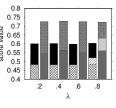
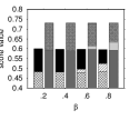
Baseline. We compare our methods against an adapted version of BestCoverage from [12] for diversified ranking over graph data so as to consider documents’ content as well. As we described in §2.2, their effort constitutes a heuristic scheme. All methods were implemented in Java and run in an AMD Opteron processor tweaked at 2.3 GHz.
5.2 Results
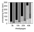
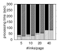
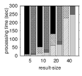
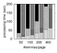
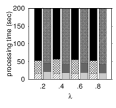
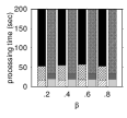
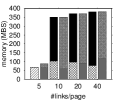
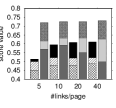
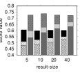
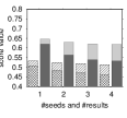
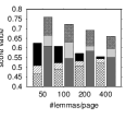
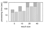
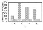
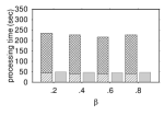
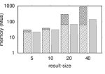
In Figures 4, 4 and 4, we present our results for the synthetic workload, whereas in Figs. 8, 8 and 4 we show our results for the Wikipedia dataset. First and foremost, a prevalent observation throughout our evaluation is that our methods clearly outperform the BestCoverage method from [12] in terms of all metrics, processing time, allocated memory, and result quality, for all configurations of our parameters. In particular, our paradigm is faster by several orders of magnitude and consumes significantly less memory. More importantly, unlike our competitor, our approach is not limited to examining web-pages up to a particular distance, and it therefore returns a result of better quality. The main reason their performance deteriorates lies with the fact that they do not traverse the graph carefully as they do not exploit the information originated from previous traversals. For instance, they consider web-pages up to a certain number of hops away from the elements of the current result, but still, the cost of computing the score of a candidate document remains high, as our evaluation confirms, since many other documents can intervene in between when trying to compute the network distance between the candidate document and every other result item. On the other hand, our scheme performs a coordinated search around each result item and the query center until certain constraints are satisfied. What is more, according to our scheme we do not have to traverse any subpath twice, not even for score computation. Remember how we expand each distance-heap and insert the new node at the respective score-heap until it is encountered from all sources. That is the moment it becomes a candidate result. Never again any part of the path to that node from any source is visited. In particular, we reckon that graph data have specific characteristics that should be carefully considered in order to design effective and efficient processing methods. We display the results for our competitor for the synthetic workload only.
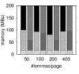
Effect of collection size . We can study the impact of the number of documents in the collection from the first column of Figs. 4, 4 and 4. Regarding execution time, we observe in Fig. 4(a) that the first phase of our paradigm, consisting of our heuristic method, requires less time than our hill-climbing approach. The first phase requires almost just as much time for both min-avg and min-max ranking criteria. However, more time is spent during the latter phase when min-avg ranking criteria are used. We observe the same pattern in Fig. 4(a) where the amount of memory allocated by each method is shown. In Fig. 4(a), the result quality seems to be only slightly affected by the size of the collection, and just for the heuristic method under min-max ranking criteria. Notably, for min-sum ranking the number of the web-documents has no effect at all.

Effect of number of hyper-links . The second column illustrates performance in terms of the number of hyper-links to other documents of the collection. Apparently, processing time grows with the number of links per document in Fig. 4(b). The reason behind this behavior lies with the fact that as the size of the collection remains the same and equal to the default value, and increasing the fan-out parameter brings the documents closer to the query center. Subsequently, we expect more documents to be examined now in order to ascertain whether they are qualified to be added to the result, and more documents will constitute candidate result items to be compared with other eligible ones. This imposes a computational overhead that is reflected in Fig. 4(b) accordingly. Fig. 4(b), the memory requirements increase for min-max criteria as expected, but especially for min-avg criteria allocated memory seems a little irregular with the fan-out degree. What could exactly cause an increase in the allocated memory? First, for our hill-climbing approach that would be the number of qualified subsets waiting to be further processed. Keep in mind that with each such subset we construct an iterator that allows us to traverse the best items to complement that particular subset. Evidently, the number of subsets that are kept simultaneously increases with the fan-out degree for min-max. However, for min-avg their number increases for the first two configurations to gradually diminish later on. In practice, the min-avg ranking function allows for more effective pruning as it enables ranking of greater granularity. More specifically, as the cardinality of the result-set increases, and has already been filled with well-diversified objects that constitute good representatives around the query center, the remaining vertices achieve scores that are almost identical regardless where they lie in the graph, for they will always have an item of the result-set somewhere relatively close, at least no further than any other vertex in the graph. We reckon that this is the critical value of the cardinality of the result-set for min-max ranking criteria, and this situation can be used as a termination criterion for the method when encountered. This is the point beyond which there is no practical distinction for that particular query center among the vertices that have been excluded from the result-set. This is also the main reason that more candidate subsets accumulate, something which is reflected on the allocated memory. This intricate detail explains most of the discrepancies in the behavior of the two ranking functions. Second, we run a configuration for our heuristic scheme where we limit the number of candidates by , with a separate seed starting from each of the most similar documents to the query center, and therefore, the memory requirements are significantly less.
Effect of result size . The third column illustrates performance in terms of the result size. Apparently, execution time grows very fast with the cardinality of the result-set in Fig. 4(c) for both phases, even though the latter phase is more expensive under min-avg ranking criteria. In Fig. 4(c), the memory allocated during the latter phase is increased compared to the amount of allocated memory during the first phase. Again, that gap is increased for min-avg ranking criteria. In Fig. 4(c), we see the scores deteriorate with , but this is only attributed to the augmentation of the result with more elements. Since those are selected incrementally, less relevant elements start to appear whose dissimilarity from the rest of the result items evidently fails to compensate for that relevance loss.
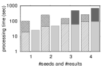
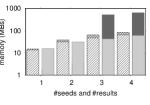

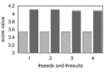

Effect of number of seeds and results . We depict in the fourth column the performance in terms of the number of seeds produced during the first phase, and the number of results returned by the second phase from which we select the best to return to the user. This is an important system parameter of our scheme that does not affect our competitor, and therefore, no results are shown for the BestCoverage method here. We also remind the reader that each of those results has cardinality defined according to the aforementioned parameter . Time grows linearly in Fig. 4(d) for min-avg ranking criteria and sub-linearly for min-max ranking criteria. We make identical remarks in Fig. 4(d) where the memory allocated by our heuristic scheme increases linearly, whereas seems to grow faster for our hill-climbing approach. In Fig. 4(d), we see the beneficial effect of this parameter where the quality of the score ameliorates. This is expected due to the wider variety of sets from which we select the final result. However, the improvement is not surprising and it indicates that even for small values of this parameter our paradigm is in position of constructing a well-diversified set. Subsequently, we claim that the time overhead stemming from increasing this parameter to large values does not compensate for the improvement in the quality of the result for our synthetic dataset. Setting this parameter to a small value (say two or three, just like we do for the default value) is sufficient.
Effect of number of lemmas . The fifth column represents our results with regard to the number of lemmas observed per web-document. For our configuration the lemma frequencies follow a zipfian distribution with skewness factor equal to . Processing time and the amount of allocated memory grow linearly with the number of lemmas in Figs. 4(e) and 4(e) as expected. In particular, we see in Fig. 4(e) that our heuristic method requires the exact amount of memory regardless the increase in the number of lemmas. This can be attributed to the fact that this measurement does not account for storing the textual descriptions themselves, which of course would now are larger and more cumbersome (for computing inner products for similarities, etc.), as the response times indicate, but only accounts for the references to those documents that each method creates. Nevertheless, we discern an irregular pattern for our second phase. These fluctuations testify the sensitivity of the latter method to this parameter. In Fig. 4(e), the scores for min-max ranking criteria tend to converge with the increase in the number of lemmas, but there is a steady advantage for min-avg ranking. The reasons for this behavior lie again with the enhanced granularity that the min-avg ranking criteria offer.
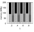
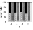
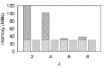
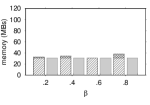
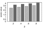
Effect of trade-off parameters and . Regarding the smoothing parameters and of the ranking function, those have little impact on either execution time, or allocated memory in Figs. 4(f), 4(g), 4(f), 4(g), for either min-avg, or min-max criteria. However, this is not true for the scores achieved in Figs. 4(f) and 4(g). In essence, applying the hill-climbing approach right after the heuristic method, improves the greedy result in a way that the heuristic method could not do. To elaborate, unlike our hill-climbing approach, the selection of the next element for the greedy method takes place in accordance with the previously selected items, without being able to undo any of the previous selections and replacing them with a better object given the selection of a subsequent element. The last row of our results signifies exactly the contribution of the latter phase to the refinement of the result. Arguably, for some configurations however, when the result of the first phase is good enough, the latter phase is not necessary, as the sets used to seed it do not lead to a subsequent better result for they are already well-diversified. Another way to interpret such a behavior would be that for those configurations, the form of the search space impedes the retrieval of better replacements, and therefore, search has to be initiated from more seeds so as to overcome this difficulty. Also, we might want to put into the same category the case where the improvement does not compensate for the time overhead. But when can we claim that the second phase is redundant, or has nothing contribute? In order to answer this question a closer look is crucial so as to detect those cases. Apparently, the only cases where the contribution of the latter phase is subliminal is when either or take low values. For every other configuration, we see that at some degree our hill-climbing approach succeeds in ameliorating the quality of the result of the heuristic method. Keep in mind that at all times is set to zero, and thus, relevance is computed by textual similarity only. In effect, when also takes low values, then diversified ranking relies substantially on the content of the web-documents and their network distances play a secondary (but still important) role in the computation of the result. Thereby, when both factors of the ranking functions (for relevance and result items’ dissimilarity) agree on what aspect of the data to leverage, then the heuristic method leaves no room for the second phase to improve the result. We observe the same phenomenon for low -values. This is when our search is oriented towards result items’ dissimilarity instead of their relevance, and since the default value of aggregating result items’ dissimilarity is directed towards elements’ network distances by convention, we tacitly compare against the case where our main concern is biased towards network characteristics in terms of relevance and result items’ dissimilarity also. Consequently, we can rely on the heuristic result exclusively when both factors agree on what aspect of the data should be put emphasis.
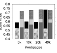
Additional remarks on the Wikipedia dataset. We show in Figs. 8, 8 and 8 our results with regard to the result-size (cardinality ), the number of seeds and results , but also the trade-off parameters of the used MMR ranking functions and , respectively. Clearly, there is a one to one association of our observations for the synthetic workload to the Wikipedia dataset throughout. The results from the two different workloads do not contradict for any configuration. Nevertheless, in the two last columns one notices that the hill-climbing method, corresponding to the second processing phase, cannot improve the intermediate result that the heuristic method produces during the first processing step. More specifically, we conclude that the default number of seeds (two in our case) is not sufficient for the second phase to find good replacements for the heuristic set collection. Notably however, when it does improve the heuristic intermediate result for larger and values, the computation overhead becomes preventive mainly to the large size of the article collection, and as a result does not seem to compensate for the improvement.
Moreover, it is hard to miss the sudden increase in memory requirements for low values in Fig. 8(c) during the latter processing phase (hill-climbing) for min-avg ranking. This configuration denotes that we are interested in dissimilar result-items mainly, rather than relevant. It looks like the competition for which subset will prevail is fierce as pruning becomes not as helpful, and this is why we have to keep the structures associated with so many subsets waiting to be refined and augmented with even better replacements. Remarkably, this spiking behavior is not present in Fig. 8(c), and this can mean only one thing. Even though there is an increased number of subsets to be processed, each of them has no more than just a few replacements eventually that can complement them, and thus, refinement is fast for each of them. In effect, since the default aggregation of content dissimilarity and network distance gives priority to the latter, graph search becomes quite limited and indicates a few good replacements within a well-bounded search space. Most importantly, owing to our verso method, this is the lossless way to bound the search space, whereas our competitor uses an artificial threshold of a fixed maximum number of hops that graph search can expand, even when all the interesting documents that achieve high scores are just a little further away from the query center. This is the most prominent advantage of our paradigm.
6 Conclusions
To recapitulate, in this paper we studied the problem of result diversification over interconnected document collections, e.g. web-pages. To the best of our knowledge our paradigm constitutes the very first approach to consider the network structure formed by the documents’ links apart from their content. Our solution relies on greedy heuristics to obtain an initial set of candidate solutions, refined through a hill-climbing approach. The criteria we adopt are based on Maximal Marginal Relevance (MMR) ranking functions which were expanded for our purposes so as to compromise objects’ network distances with their content similarities according to their textual descriptions. Withal, special parameters can be used to configure the trade-off of one feature over the other, in such a way that the users’ preferences can be accommodated to the utmost degree. Several optimizations have been employed in our paradigm so as to make feasible the processing of large graphs. Moreover, our elegant design allows for the tweaking of the response times when required, sometimes at a loss over the result quality if necessary. Finally, a thorough and meticulous experimental evaluation validates the effectiveness and efficiency of our method. Last but not least, we launched a prototype implementing our methods. It runs over the Wikipedia dataset but can be extended with other document collections, as well.
References
- [1] R. Agrawal, S. Gollapudi, A. Halverson, and S. Ieong. Diversifying search results. In WSDM, pages 5–14, 2009.
- [2] G. Călinescu, C. Chekuri, M. Pál, and J. Vondrák. Maximizing a monotone submodular function subject to a matroid constraint. SIAM J. Comput., 40(6):1740–1766, 2011.
- [3] J. G. Carbonell and J. Goldstein. The use of MMR, diversity-based reranking for reordering documents and producing summaries. In SIGIR, pages 335–336, 1998.
- [4] C. L. A. Clarke, M. Kolla, G. V. Cormack, O. Vechtomova, A. Ashkan, S. Büttcher, and I. MacKinnon. Novelty and diversity in information retrieval evaluation. In SIGIR, pages 659–666, 2008.
- [5] M. Drosou and E. Pitoura. Search result diversification. SIGMOD Record, 39(1):41–47, 2010.
- [6] M. Drosou and E. Pitoura. Disc diversity: result diversification based on dissimilarity and coverage. PVLDB, 6(1):13–24, 2012.
- [7] M. Drosou and E. Pitoura. Multiple radii disc diversity: Result diversification based on dissimilarity and coverage. ACM Trans. Database Syst., 40(1):4, 2015.
- [8] P. Fraternali, D. Martinenghi, and M. Tagliasacchi. Top-k bounded diversification. In SIGMOD, pages 421–432, 2012.
- [9] S. Gollapudi and A. Sharma. An axiomatic framework for result diversification. IEEE Da. Eng. Bul., 32(4):7–14, 2009.
- [10] J. R. Haritsa. The KNDN problem: A quest for unity in diversity. IEEE Data Eng. Bull., 32(4):15–22, 2009.
- [11] J. He, H. Tong, Q. Mei, and B. K. Szymanski. Gender: A generic diversified ranking algorithm. In NIPS 2012, pages 1151–1159, 2012.
- [12] O. Küçüktunç, E. Saule, K. Kaya, and Ü. V. Çatalyürek. Diversified recommendation on graphs: pitfalls, measures, and algorithms. In WWW 2013, pages 715–726, 2013.
- [13] R. Li and J. X. Yu. Scalable diversified ranking on large graphs. IEEE Trans. Knowl. Data Eng., 25(9):2133–2146, 2013.
- [14] Z. Liu, P. Sun, and Y. Chen. Structured search result differentiation. PVLDB, 2(1):313–324, 2009.
- [15] Q. Mei, J. Guo, and D. R. Radev. Divrank: The interplay of prestige and diversity in information networks. In SIGKDD 2010, pages 1009–1018, 2010.
- [16] G. L. Nemhauser, L. A. Wolsey, and M. L. Fisher. An analysis of approximations for maximizing submodular set functions - I. Math. Program., 14(1):265–294, 1978.
- [17] L. Page, S. Brin, R. Motwani, and T. Winograd. The pagerank citation ranking: Bringing order to the web. Technical Report 1999-66, Stanford InfoLab, November 1999.
- [18] H. Tong, J. He, Z. Wen, R. Konuru, and C. Lin. Diversified ranking on large graphs: An optimization viewpoint. In SIGKDD 2011, pages 1028–1036, 2011.
- [19] G. Tsatsanifos. The tantalizing new prospect of index-based diversified retrieval. In SIGMOD/PODS 2013 Ph.D. Symposium, pages 49–54, 2013.
- [20] G. Tsatsanifos, D. Sacharidis, and T. Sellis. RIPPLE: A scalable framework for distributed processing of rank queries. In EDBT 2014, pages 259–270, 2014.
- [21] E. Vee, J. Shanmugasundaram, and S. Amer-Yahia. Efficient computation of diverse query results. IEEE Data Eng. Bull., 32(4):57–64, 2009.
- [22] M. Vieira, H. Razente, M. Barioni, M. Hadjieleftheriou, D. Srivastava, C. Jr., and V. Tsotras. On query result diversification. In ICDE, pages 1163–1174, 2011.
- [23] Y. Xu and H. Yin. Novelty and topicality in interactive information retrieval. JASIST, 59(2):201–215, 2008.
- [24] C. Yu, L. V. S. Lakshmanan, and S. Amer-Yahia. It takes variety to make a world: Diversification in recommender systems. In EDBT, pages 368–378, 2009.
- [25] C. Zhai, W. W. Cohen, and J. D. Lafferty. Beyond independent relevance: Methods and evaluation metrics for subtopic retrieval. In SIGIR, pages 10–17, 2003.
- [26] M. Zhang and N. Hurley. Avoiding monotony: Improving the diversity of recommendation lists. In RecSys.
- [27] Y. Zhang, J. P. Callan, and T. P. Minka. Novelty and redundancy detection in adaptive filtering. In SIGIR, pages 81–88, 2002.
- [28] X. Zhu, A. B. Goldberg, J. V. Gael, and D. Andrzejewski. Improving diversity in ranking using absorbing random walks. In HLT 2007, pages 97–104, 2007.
- [29] C.-N. Ziegler, S. M. McNee, J. A. Konstan, and G. Lausen. Improving recommendation lists through topic diversification. In WWW, pages 22–32, 2005.