Classical and quantum particle dynamics in univariate background fields
Abstract
We investigate deviations from the plane wave model in the interaction of charged particles with strong electromagnetic fields. A general result is that integrability of the dynamics is lost when going from lightlike to timelike or spacelike field dependence. For a special scenario in the classical regime we show how the radiation spectrum in the spacelike (undulator) case becomes well-approximated by the plane wave model in the high energy limit, despite the two systems being Lorentz inequivalent. In the quantum problem, there is no analogue of the WKB-exact Volkov solution. Nevertheless, WKB and uniform-WKB approaches give good approximations in all cases considered. Other approaches that reduce the underlying differential equations from second to first order are found to miss the correct physics for situations corresponding to barrier transmission and wide-angle scattering.
I Introduction
Strong fields provide new opportunities for measuring unobserved processes both within the Standard Model and beyond. Scattering amplitude calculations for these processes require dressed particle wavefunctions in order to describe the interaction with the strong (background) field. Due to the high field strengths involved, however, the wavefunctions cannot be constructed using the standard method of perturbation in the coupling. Thus one must either use nonperturbative approximations, or work with special cases where exact solutions exist.
The latter situation is typified by intense laser-matter interactions (for introductions and reviews see Ritus ; Marklund:2006my ; Heinzl:2008an ; Gies:2008wv ; Dunne:2008kc ; DiPiazza:2011tq ; King:2015tba ), where the plane wave model of a laser field allows for a fully analytical treatment Volkov ; Reiss:1962 ; Nikishov:1963 ; Nikishov:1964a ; Narozhnyi:1964 ; Goldman:1964 ; Kibble:1965zza . The model is powerful but restrictive, being unable to account for effects due to the spatial geometry of a realistic laser pulse. This limits our ability to predict and analyse experimental results – indeed the primary source of phenomenological results for the complex interactions of focussed laser fields with electron bunches and solid targets are PIC-simulations, reviewed in Gonoskov:2014mda .
In order to gain analytical insights, confirm numerical results, and improve experimental predictions, we must go beyond the plane wave model Mendonca ; Raicher:2013cja ; DiPiazza:2013vra ; Oertel:2015yma . This task is as challenging as it is open-ended. We therefore approach it here by restricting ourselves to a specific class of extensions beyond the plane wave model, by retaining the single-variable () field dependence, but generalising from lightlike to arbitrary .
There are only three Lorentz-inequivalent cases. For we have plane waves, and both the quantum and classical dynamics are integrable in the sense that the classical equations of motion, as well as the Dirac and Klein-Gordon equations, are exactly solvable due to the presence of sufficiently many conserved quantities. may describe an undulator Jackson:1998nia or a plane wave in a medium with refractive index Cronstrom:1977 , depending on the chosen or, equivalently, the chosen frame: these two systems are boost-equivalent. Similarly, can describe a plane wave in a medium of refractive index Cronstrom:1977 ; Becker:1977 , or a time-dependent electric field, depending on the chosen frame Bulanov:2003aj . The latter case can also be obtained by restricting to a magnetic field node of a standing wave depending on two lightfront variables.
For there are no general solutions to the Klein-Gordon or Dirac equations. When building approximate solutions there are broadly two approaches to consider. Either one can look for general approximations, which hold for all field shapes as the Volkov solution for plane waves does Volkov , or one can look for approximations specific to a particular field shape. In the case of both the former Mendonca and latter Raicher:2013cja ; Raicher:2015ara ; Raicher:2016bbx have recently begun to attract attention. Here we will mainly focus on the case . The approaches we describe can also be applied to , although the physics is different Becker:1977 . For an analysis of the Klein-Gordon equation in this case, in the context of standing waves, see Hu:2015 .
We will consider several different approaches to the problem of building accurate approximations, examine the connections between them, the situations in which they are applicable, and their sensitivity to kinematic parameters and field shape.
This paper is organised as follows. We begin in Sect. II with a classical comparison of particle dynamics in fields with and . We compare the emission spectra for electrons in a laser and in an undulator, and explain why the spectra are similar in the high-energy limit, despite the two cases being Lorentz-inequivalent. In Sect. III we turn to the quantum problem, which is to solve the Klein Gordon equation in the chosen background field (we consider only scalar QED, for simplicity). We review existing approaches and present an approach based on ‘reduction of order’ as applied by Landau and Lifshitz to radiation reaction. In Sect. IV we consider a different approach: by rewriting the Klein-Gordon equation as a Schrödinger equation we are able to use intuition from quantum mechanics to develop accurate approximate wavefunctions. Examples for incoming and outgoing scattering states are given. We use the intuition built up from this in Sect. V to re-analyse the literature and reduction of order approaches. We conclude in Sect. VI.
II Classical dynamics: lightlike vs. spacelike field dependence
The field strength of our background is
| (1) |
where , and the define the shape and amplitude of the field. For (1) describes a plane wave (in all frames). For , we can go to a frame where , in which case (1) describes a static but position-dependent magnetic field as may be found in an undulator. If we then boost along , and in this frame (1) describes a plane wave propagating in a medium with refractive index Cronstrom:1977 ; Becker:1977 . Similarly, for we can take , which describes a time-dependent but homogeneous electric field, and boosting gives a plane wave in a medium with .
As the frequencies in the boosted frames increase and approaches , i.e. the refractive index approaches unity. However, the plane wave case cannot be recovered by boosting, as is invariant. This is made explicit by introducing the boost rapidity , which enables us to write, for ,
| (2) |
The ‘lightlike limit’ would correspond to dropping the second term in (2), whereupon would vanish. As this cannot be achieved with a boost, the emission spectra from e.g. charges in undulators and charges in lasers cannot be equivalent Harvey:2012ie . However, the spectra do become similar at e.g. high energy, or for large boosts, because even though is invariant, the contraction of with other vectors can clearly be dominated by the first term in (2). Let us then compare the emission spectrum of an electron in fields with and .
The spectral density of radiation with momentum () is
| (3) |
where is the Fourier-transformed classical current. The notation refers to the fact that the spectral density becomes the average number of emitted photons in QED. In terms of proper time , orbit and kinetic momentum of the emitting particle, the current is
| (4) |
Hence the classical orbit is required. Writing the Lorentz equation in the field (1) has the first integral
| (5) |
in which the ‘work done’ by the field is
| (6) |
is the momentum at some chosen and
| (7) |
The sign of is determined by the condition that as we turn the field off, and the ‘potential’ has the same form as in the plane wave case. Note that the momentum is at this stage only an implicit function of : we also need to identify as a function of by solving the equation
| (8) |
which amounts to performing part of the second integration to obtain the orbits. (Unlike in the plane wave case, is not conserved.) This can be done analytically only for special choices of and kinematics (see below). The condition that restricts the range of positions accessible by the particle. The trajectory may be parameterised by only if the discriminant in is positive for all : is then a monotonic function and we may trade for . By taking via e.g. a coordinate rotation Hornbostel:1991qj ; Ji:2001xd ; Ji:2012ux ; Ilderton:2015qda (not a boost), (5), (7) and (8) reduce to and
| (9) |
which can straightforwardly be integrated again and yields the charge orbit motion in a plane wave Landau:1982dva ; Sarachik:1970ap .
In order to make a connection with some of the examples below, in the quantum theory, consider the particular but familiar case of a head-on collision between an electron and a monochromatic, circularly polarised field111This case should be considered as the infinite duration limit of a long pulse, just as for the plane wave case, see Kibble:1965zza .; in the frame where , this is the field of a helical wiggler Alferov:1979tp . In this case is constant,
| (10) |
and the classical equation of motion is integrable, assuming parameters such that the discriminant is positive. The calculation of the spectral density is very similar to that in (LL-QED, , §101), so we skip to the final result. This is
| (11) |
where , is the emission angle relative to , the cycle-averaged (“quasi”) momentum is
| (12) |
and
| (13) |
As in the plane wave case, periodicity results in a spectrum composed of discrete harmonics labelled by integer , and defined by the support of the delta function in (11) which, we observe for later, depends on the quasi-momentum (12).
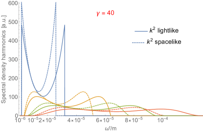
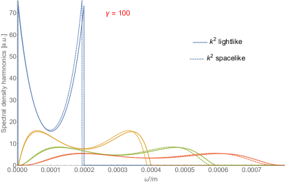
The lightlike limit takes , and by inspection of (7)-(13) we can see that differentiates between the cases and . If is made large, so that rather than , then particle dynamics and hence the emission spectrum will be very different in the two fields. (Further, we can take when , which also suggests large differences because is always positive in the plane wave case.) However when is sufficiently small such that , we can define an ‘equivalent’ plane wave field for which the emission spectrum will almost match that of an undulator, by specifying the invariants and . To illustrate, take , and for the static magnetic field. For the plane wave we take and choose the frequencies such that is the same in both systems. This requires
| (14) |
(We write equivalent ‘plane wave’ rather than ‘laser’ because, in contrast to (14), laser frequencies are much larger than the frequencies associated with the geometry of undulators. For an optical laser eV, while for an undulator with period of order cm, the frequency is eV.) A comparison of the emission spectra in the monochromatic field, for two values of , is shown in Fig. 1. For the lower value, , we have and there is a clear difference – both the amplitudes and ranges of the spectral harmonics differ between the two cases. For the higher energy of however, we have and the two spectra are almost in agreement.
The assumptions of a head-on collision and a periodic field Raicher:2013cja give a well understood system and a testing ground for new approaches, but on the other hand represent an oversimplified special case. Once we allow for general the classical motion is described not by simple sinusoidal functions but by more involved elliptic functions. Similarly, nontrivial field envelopes increase the complexity of both the physics (e.g. the emission spectrum) and the calculations. All of these aspects will come into play in the quantum theory, to which we now turn.
III First-order approaches to the quantum problem
The problem to solve in the quantum theory is the identification of the wavefunctions which describe incoming and outgoing electrons and positrons, for use in scattering calculations. In scalar QED these wavefunctions are solutions of the Klein-Gordon equation
| (15) |
where is the background-covariant derivative, and where the gauge potential can be chosen as . Current approaches to solving (15) mimic that used in the plane wave case, by making the ansatz where Mendonca ; Raicher:2013cja . With this the Klein-Gordon equation reduces to
| (16) |
For this is a first-order equation which immediately yields the Volkov solutions. For all the equation is second order, and there is no general solution because of the arbitrarily varying prefactor of , a non-constant coefficient akin to the potential in the Schrödinger equation. As the difficulty here comes from the fact that the equation (16) is second order, we begin by discussing a variety of approaches which seek to reduce (16) to a first-order equation.
III.0.1 Perturbation theory and a slowly varying envelope approximation
For plane waves with , the solution to (16) is Volkov
| (17) |
If we are interested in ‘perturbing around’ the plane wave solution, then perturbation in would seem to be a natural approach. However, in the frame where or for respective , perturbation in clearly corresponds to a low-frequency expansion, whereas the Volkov solution (17) makes no assumption about the frequency scale, and indeed is, using (7), nonperturbative in .
Of course has dimensions, so we need a second scale to compare against in order to develop a meaningful expansion in a dimensionless parameter. The approach of Mendonca is to make a slowly varying envelope approximation which, in our notation and made covariant, reads
| (18) |
From this, one can identify dimensionless as a potential expansion parameter (the factor of 2 is for later convenience). Using perturbation in then corresponds, at lowest order, to dropping the double-derivative term in (16). The resulting first-order equation is immediately integrable and the solution is formally identical to the Volkov solution (17) but with spacelike or timelike, rather than lightlike:
| (19) |
III.0.2 First-order approximation
A different approach is given in Raicher:2015ara ; Raicher:2016bbx , but only for a specific field shape (monochromatic, and circular polarisation, as above). The idea is again to replace (15) with a soluble first-order equation. The choice of this equation is motivated by taking its derivative, and showing that it reproduces (15) up to terms small in some parameter. In Raicher:2015ara ; Raicher:2016bbx the parameter is,
| (20) |
where the last identity holds in the frame where , introducing . A small means that the particle’s initial transverse momentum should be much smaller than the total energy, and the field strength. This approach has the potential to be applied to other field shapes.
III.0.3 Reduction of order
We present now an alternative method which combines the perturbative approach above with that in Raicher:2015ara ; Raicher:2016bbx : we again look for an ‘effective’ first-order equation, but related to an expansion in the small parameter . Observe that dividing (16) by makes the coefficients dimensionless, and the equation becomes
| (21) |
If is a small parameter then (21) constitutes a typical example of singular perturbation theory Bender:1978 , in which the highest derivative term is multiplied by the small parameter. This situation is familiar from the study of radiation reaction in strong fields, where the third-derivative term in the Lorentz-Abraham-Dirac (LAD) equation L ; A ; D is a singular perturbation in the same sense as encountered here. We therefore apply the Landau-Lifshitz approach Landau:1982dva to our problem. This means using recursion: taking another derivative of, and employing, (21) yields
| (22) |
Plugging this into (21) and discarding terms of order and higher again leaves a first-order equation,
| (23) |
(This approach can be extended directly to include higher orders of in (23).) This is a non-singular perturbation of the plane-wave equation which is still reproduced in the limit . The solution to (23) is
| (24) |
For we recover (19) for any value of (so, again, this is not an expansion ‘around’ the plane wave case).
Using ‘reduction of order’ (RO) we thus obtain a wavefunction which is no more or less complicated than the Volkov solution and which, like Volkov, applies for any field shape. We refer to this as a ‘partial resummation’ of the perturbative series because although we have thrown away terms of order from the equation (23), the solution (24) contains all orders in .
RO is not completely general because, for spacelike, and therefore can be of any sign and size (in the ‘undulator frame’, for example, ). When is not small, the arguments leading to RO do not hold.
IV Second-order approaches to the quantum problem
The approaches above try to solve the problem at hand based on experience of the plane wave case, hence the focus on eliminating the second derivative in (16). It is however not obvious that this is the best approach to take. For example, the dimension of the solution space changes from two to one when going from second to first-order, which can correspond to the decoupling of states from a theory Heinzl:2007ca ; it is not clear apriori that these states should be discarded.
Consider then the Schrödinger equation. This is a well-understood second order equation in quantum physics where the second derivative term is retained despite being multiplied by a parameter (Planck’s constant) considered ‘small’ in the semi-classical limit. In this section we therefore rewrite the Klein Gordon equation (15) as a Schrödinger equation, and use intuition from quantum mechanics to gain insight into its solutions and into finding physically-motivated approximations.
Ultimately we are still interested in solutions with scattering boundary conditions, i.e. which go like asymptotically, so that the solution is free far from the field, but we make an ansatz
| (25) |
Compared to the ansatz in Sect. III, this simply moves all -dependence in into the unknown function . (This new ansatz corresponds to transforming (21) to “normal form” Polyanin:1994 using a Galilei boost to remove the first derivative term.) The Klein-Gordon equation then becomes
| (26) |
which we recognise as a Schrödinger equation for ,
| (27) |
and the first task is to map (26) to (27) by identifying the form and relative sizes of the potential , the energy eigenvalue and the analogue of . We will now see through three examples that this identification and the corresponding approximate solutions to (27) depend sensitively on both the parameters and the background field shape.
IV.1 Example 1: over the barrier
For a general scattering amplitude we need both incoming and outgoing states. Consider first the case of incoming particles, incident on the field (1). We have and contains the typical frequency scale of the background. Write the field as where is the amplitude and is of order unity. In addition to taking small, the typical case of interest for incoming particles is a nearly head-on collision, so that . We also assume i.e. that the initial transverse momentum is much smaller than the typical transverse momentum acquired in the field. Then taking (26) and dividing by we identify
| (28) |
of order unity and
| (29) |
so that small corresponds to the semiclassical limit. We begin by assuming that the dimensionless field strength is much lower than the particle energy , so that
| (30) |
Comparing (30) and (28) shows that this situation is analogous to over the barrier scattering in quantum mechanics. As such the natural approximation with which to solve (27) is semiclassical WKB Bender:1978 :
| (31) |
The sign may be fixed either by boundary conditions on at , or by the limit. The WKB wavefunction is based on making a free-field ansatz, and works well in the case that the particle is almost free due to its high energy Bender:1978 , independent of the precise form of the potential .
IV.2 Example 2: wide-angle scattering/under the barrier
Quantum effects can cause wide-angle particle scattering, where classical motion cannot Green:2013sla . In this case the assumptions which are natural for incoming particle states (high energy, nearly head-on) break down, and one must instead consider large transverse momenta. In this case the Schrödinger equation may describe, in contrast to the above, a below-the-barrier scattering problem.
To illustrate we use the Sauter pulse with gauge potential ( as in (1))
| (32) |
For this would correspond to a short, subcycle laser pulse. We again write , with as above. The field can give a classical particle a transverse momentum of order , so we measure in these units, writing . With this the Klein-Gordon equation again reduces to a Schrödinger equation
| (33) |
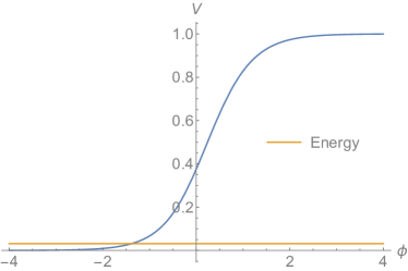
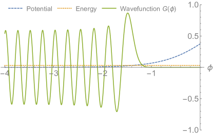
and we read off , and as above (possibly after dividing by some -dependent constant in order to normalise the potential to ). To impose the condition of wide-angle scattering we take of order unity, and , which corresponds to the longitudinal momentum being much smaller than the transverse momentum. Thus the eigenvalue now obeys , as opposed to in the case of near-forward collisions considered above. An example is shown in Fig. 2 for . As varies, can change sign, which means we have a barrier penetration, or tunnelling problem. This suggests using a uniform WKB (“U.WKB”) ansatz for the wavefunction, of which ordinary WKB is a special case. We make the U.WKB ansatz Cherry ; MillerGood ; Miller
| (34) |
and expand as a series in . (This ansatz, used by Sauter to study the behaviour of an electron in a homogeneous field Sauter31 , gives the exact solution in a linear potential.) To lowest order the equation to solve is
| (35) |
which has the two solutions
| (36) |
In our case the integral in (36) can be performed analytically, but is an unrevealing combination of hyperbolic functions. This gives two independent solutions to (33). (Equivalently, one can use only but include both Ai and Bi terms in the ansatz for DLMF:AIRY .) Demanding that the wavefunction is continuous at the turning point and that its amplitude does not diverge asymptotically then determines the solution.
The result is plotted in Fig. 2. The wavefunction is real, and is indistinguishable from a numerical solution of the ODE (33) on the scales shown, demonstrating the accuracy of the approach. Importantly, the U.WKB wavefunction clearly reproduces the expected physics: when above the barrier and the wavefunction is oscillatory, but when under the barrier and the wavefunction is exponentially damped. In Sect. V.1 we will compare these results with those obtained from the first-order approximations.
IV.3 Example 3: periodic fields and the Mathieu equation.
For our final example we return again to the case of monochromatic, circularly polarised fields. The Klein-Gordon equation for then becomes equivalent to the Mathieu equation DLMF ; Muller-Kirsten:2012wla
| (37) |
with the identifications and Cronstrom:1977 ; Becker:1977
| (38) |
Despite the apparent simplicity of the classical theory, the quantum theory exhibits an intricate nonperturbative structure for Bender:1978 ; Dunne:2016qix . The – parameter space of solutions can be divided into ‘bands’ and ‘gaps’; for parameters in the gaps, the solutions to (37) increase exponentially with (or ) and cannot be normalised, so must be discarded as unphysical Cronstrom:1977 ; Becker:1977 . For a recent discussion of the band structure in the language of resurgence, see Dunne:2016qix and references therein.
To map the Mathieu equation to the Schrödinger equation (27) note that contains now a constant term, which we move into the eigenvalue, identifying
| (39) |
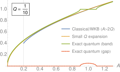
These identifications differ from those used in the examples above, illustrating the dependence of the system, approach, and solutions on the form of the potential. To understand how the parameters affect the physics, it is convenient to focus on a particular observable, for which we choose the quasi-momentum. Classically, this is just the cycled-averaged particle momentum. Quantum mechanically, it can be identified as the cycle-average of the exponent of the wavefunction. The frequencies of photons emitted by an electron in our field are determined by the conservation of quasi-momentum according to
| (40) |
where () is the quasi-momentum of the incoming (outgoing) electron and is the emitted photon momentum; (40) is familiar from the plane wave case LL-QED . In the classical limit, and for e.g. a head-on collision, (40) becomes equivalent to the support of the delta function in (11).

The exact form of the quasi-momentum in the quantum case is known Cronstrom:1977 ; Becker:1977 : using the notation of Becker:1977 we have
| (41) |
where is the ‘Mathieu characteristic exponent’ DLMF . The bands, i.e. the spaces of physical solutions, are defined by the condition Cronstrom:1977 ; Becker:1977 ; DLMF . The exact result (41) can be compared with the approximations above. The WKB wavefunction gives the quasi-momentum as (41) but with
| (42) |
in which is the complete Elliptic integral of the second kind. The exact result and WKB approximation in (42) are plotted and compared in Fig.’s 3 and 4. If is large, so that is small, we are in a semiclassical regime where WKB applies. The WKB wavefunction gives good agreement in this case, for , see Fig. 3. Observe that precisely when so that the energy eigenvalue lies above the potential. For we are within the potential, and there is a rich structure of bands and gaps even when because of quantum effects from . However, if is small, then is large, which is a strong coupling limit Dunne:2016qix . In this case a direct small- approximation Becker:1977 ; DLMF ,
| (43) |
gives a better approximation both above and below the barrier than the WKB approximation, as shown in Fig. 4.
V Comparison of first and second order approaches
Having built up some intuition, we re-analyse the first-order approaches discussed in Sect. III.
V.1 Reduction of order revisited
We begin by rewriting the RO equation (16) in the second order, Schrödinger equation notation of Sect. IV:
| (44) |
where the sign is minus that of . It is easily confirmed that a straightforward perturbative expansion in gives only the trivial solution ; this is consistent with the results in Sect. IV where we saw that the leading behaviour of the wavefunctions is non-perturbative in . Each derivative in (44) comes with a factor of ; temporarily scaling this out by sending will allow us to better compare the relative sizes of the first and second derivative terms. Writing a dot for a derivative with respect to the new variable, (44) becomes
| (45) |
Recalling that is of order unity, the only candidate small parameter is . Hence recursion in the second-derivative term corresponds to a large expansion. This is confirmed by also rewriting the RO wavefunction (24) in the Schrödinger equation notation (returning to the usual variable),
| (46) |
and observing that is the third order expansion of the exponent of the WKB solution (31) in powers of , in the limit that is very much greater than . Expanding the square root in (31) gives the phase needed to convert from to , and the terms under the integral in (46) and re-exponentiating the prefactor in (31) gives a term in the exponent, the lowest order expansion of which gives the final term in (46). The expansion holds when the energy is far above the potential, , therefore RO is a high-energy approximation. This is consistent with the perturbative result obtained by dropping the double derivative term: the lowest order perturbative wavefunction (19) is a phase, as expected for above the barrier wavefunctions, but which can never describe barrier penetration (or potential well/bound state) problems where the solutions are asymptotically damped.
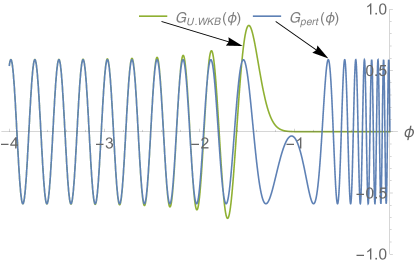
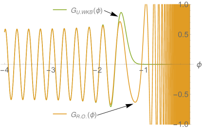
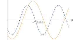
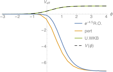
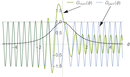
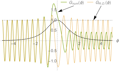
Hence RO, and by extension the perturbative approach, gives an approximation of a WKB ansatz which is appropriate for ‘above the barrier’ parameters. A further interpretation can be acquired by employing multi-scale perturbation theory Bender:1978 . In this approach, RO captures the physics on only the shortest timescale and misses physics on the longer timescale associated with the second derivative. RO is therefore unlikely to accurately reproduce under-the-barrier physics. We confirm this in Fig. 5 and Fig. 6, where we compare the perturbative, RO and U.WKB wavefunctions for the example of Sect. IV.2. We plot in all cases, obtained from by multiplying by a phase. Note that the U.WKB wavefunction is a superposition of perturbative or RO wavefunctions obtained by summing contributions from for a given . Normalisations are fixed by matching the asymptotic behaviour of the wavefunctions where the potential vanishes, and where they all agree. The general behaviour is the following. The three wavefunctions agree well when . As we approach the turning point, first the perturbative wavefunction and then the RO wavefunction diverge from the U.WKB and numerical results, see Fig. 6 for details. Beyond the turning point, under the barrier, the U.WKB wavefunction is exponentially damped, as it should be. Both the RO and perturbative wavefunctions continue to oscillate under the barrier but with a lower frequency. The perturbative wavefunction, being a phase, has the same amplitude above and below, while the amplitude of the RO wavefunction grows significantly under the barrier.
These behaviours are unphysical. Their origin is efficiently captured by examining how well the Schrödinger equation is satisfied through consideration of an effective potential ‘seen’ by the wavefunction, defined by
| (47) |
For an exact solution we have , from (27). The effective potentials seen by the perturbative, RO and U.WKB wavefuntions are plotted in Fig. 7 . Both the perturbative and RO effective potentials become negative to the right of the turning point, and asymptote to a value far below, rather than above, the energy eigenvalue. This explains why the wavefunctions oscillate more quickly under the barrier: take so that the effective potentials are flat and negative, then the particles see themselves as much further above the potential than they were for , as the effective , and hence the wavenumber, or frequency of oscillation, increases. The particularly rapid oscillations seen in the RO case are explained by the very large change in amplitude of the effective potential, due to the real exponential factor in (24). This is an artefact of the approximation, in particular of expanding the prefactor of the WKB wavefunction.


V.2 Barrier transmission
Another situation in which the approximations can be tested against the well-understood physics of the Schrödinger equation is barrier transmission. We take the background field to be of sech form:
| (48) |
For as in Sect. IV.2, with , we identify
| (49) |
and has the form of a potential hill with a peak amplitude of unity.
For the parameters in Fig. 8, the energy is just below the potential peak, so that transmission of the particle through the barrier is classically-forbidden, but only just. We compare the first-order approaches with an exact numerical solution of the Schrödinger equation. Initial conditions are chosen such that all wavefunctions agree for where the potential vanishes. While the numerical solution shows reduced transmission as expected, the first-order approaches predict complete transmission through the barrier, in that the amplitudes of the approximate wavefunctions both to the left and right of the potential hill are equal. This suggests that unitarity is violated, and confirms that the first-order approximations are unable to capture the full physics.
V.3 Current conservation
Making an analogy with the Schrödinger equation has proven useful in analysing the physical content of the approximate wavefunctions above, but we can also consider observables directly, as in Sect. IV.3. Consider then the current, for a general field shape, and again in the case that the discriminant in (8) is always positive, i.e. we are above the barrier. The classical current is then
| (50) |
where the delta function is just the product of deltas in the three directions orthogonal to . We can compare this to the field theory current,
| (51) |
calculated using the various approximate wavefunctions above. Using the perturbative, RO, and WKB approximations gives
| (52) |
Neglecting overall normalisations, the WKB wavefunction recovers the classical current222The delta functions in the classical current would be recovered upon using suitably normalised wavepackets of solutions to the Klein-Gordon equation., while the RO and perturbative wavefunctions give only approximations to it. Higher-order WKB will add quantum corrections to the current. This should be contrasted with the WKB-exact plane wave case, where the classical and quantum currents are equal up to normalisation.
For the WKB, RO and perurbative wavefunctions, we observe that current conservation can be expressed as
| (53) |
For over-the-barrier parameters, we note that the classical, and therefore WKB, currents are conserved, since
| (54) |
Both the perturbative and RO methods violate this conservation. We have
| (55) | ||||
| (56) |
so that the current is conserved only up to a certain order in , consistent with (45).
VI Conclusions
We have examined a variety of methods of analysing the classical and quantum dynamics of charges in electromagnetic backgrounds depending on a single variable , where may be lightlike, timelike or spacelike. The lightlike case has been the focus of great interest for over 50 years as it corresponds to the plane wave model of intense laser fields. The classical dynamics is then integrable (the Lorentz force equation is exactly soluble), as is the quantum dynamics (through the WKB-exact Volkov solutions of the Klein-Gordon and Dirac equations). This integrability is lost upon relaxing the null-vector condition , however. There are many physical scenarios corresponding to . The timelike case, , is Lorentz equivalent to a time-dependent, spatially homogeneous electric field, while the spacelike case, , is equivalent to a static but inhomogeneous magnetic field.
We have first analysed classical dynamics in the spacelike case. There are three momentum conservation laws corresponding to translation invariance in the coordinates different from . This, together with the mass-shell constraint, is sufficient to guarantee the existence of a first integral which expresses the particle momentum as a function of . However, in contrast to the lightlike case, the appearance of a square root non-linearity means that a second integration to obtain the particle orbits is only possible in special cases. Hence abandoning the plane wave nature of the background destroys integrability despite the fact that the number of (translational) symmetries is maintained. We have discussed a special, solvable, case by comparing the electron radiation spectrum in a helical wiggler () with that in a plane wave or laser (). Despite the two spectra becoming almost identical in the high energy limit, , there is an intermediate energy range where and the spectra are significantly shifted. This is particularly relevant to simulations of electromagnetic cascades in laser backgrounds, which often adopt a (constant crossed) plane wave model at the magnetic node of a standing wave () Bell:2008ppp ; Mironov:2009cr ; Nerush:2011pp ; King:2013pp . For example, the nonlinear Compton scattering stage of a cascade becomes probable for in an optical field with intensity parameter .
In the quantum regime, the WKB method ceases to be exact when so that there is no analogue of the Volkov solution. Nevertheless, approximations based on WKB and uniform-WKB approaches work well – these are based on physical arguments, agree very well with numerics, and also produce the expected physics. The optimal uniform-WKB ansatz depends strongly both on field shape and parameters.
We have also considered perturbation theory in kinematically small parameters, leading to the use of ‘reduction of order’, familiar from the study of radiation reaction. This is a general approach in that it does not make reference to the shape of the background field considered. This seems like a promising method of generalising the Volkov solution, at least approximately, but we have seen that it is essentially a high energy approximation Blankenbecler:1987rg which is limited to ‘above the barrier’ type problems. This is particularly relevant in the context of laser-matter interactions, where reduction of order is implicitly invoked whenever the Lorentz-Abraham-Dirac equation is replaced by that of Landau and Lifshitz, and suggests that reduction of order should be further investigated in order to establish its range of validity.
Acknowledgements.
A.I. thanks Gerald Dunne for useful discussions, and the Centre for Mathematical Sciences, Plymouth University, for hospitality. A.I. is supported by the Olle Engkvist Foundation, contract 2014/744, and the Lars Hierta Memorial Foundation, grant FO2015-0359.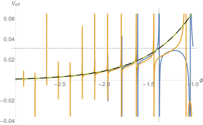
References
- (1) V. I. Ritus, J. Russ. Laser Res. 6 (1985) 497–617
- (2) M. Marklund and P. K. Shukla, Rev. Mod. Phys. 78 (2006) 591 [hep-ph/0602123].
- (3) T. Heinzl and A. Ilderton, Eur. Phys. J. D 55 (2009) 359 [arXiv:0811.1960 [hep-ph]].
- (4) H. Gies, Eur. Phys. J. D 55 (2009) 311 [arXiv:0812.0668 [hep-ph]].
- (5) G. V. Dunne, Eur. Phys. J. D 55 (2009) 327 [arXiv:0812.3163 [hep-th]].
- (6) A. Di Piazza, C. Muller, K. Z. Hatsagortsyan and C. H. Keitel, Rev. Mod. Phys. 84 (2012) 1177 [arXiv:1111.3886 [hep-ph]].
- (7) B. King and T. Heinzl, High Power Laser Science and Engineering, 4, e5 (2016) [arXiv:1510.08456 [hep-ph]].
- (8) D. Volkov, Z. Phys. 94 (1953) 250.
- (9) H. R. Reiss, J. Math. Phys. 3 (1962) 59.
- (10) A. I. Nikishov and V. I. Ritus, Zh. Eksp. Teor. Fiz. 46 , 776 (1963).
- (11) A. I. Nikishov and V. I. Ritus, Zh. Eksp. Teor. Fiz. 46, 1768 (1964).
- (12) N. B. Narozhnyi, A. Nikishov, and V. Ritus, Zh. Eksp. Teor. Fiz. 47, 930 (1964).
- (13) I. I. Goldman, Phys. Lett. 8, (1964) 103.
- (14) T. W. B. Kibble, Phys. Rev. 138 (1965) B740.
- (15) A. Gonoskov et al., Phys. Rev. E 92 (2015) 023305 [arXiv:1412.6426 [physics.plasm-ph]].
- (16) J. T. Mendonca and A. Serbeto, Phys. Rev. E 83 (2011) 026406
- (17) E. Raicher and S. Eliezer, Phys. Rev. A 88, 022113 (2013) [arXiv:1306.0486 [physics.plasm-ph]].
- (18) A. Di Piazza, Phys. Rev. Lett. 113 (2014) 040402 [arXiv:1310.7856 [hep-ph]].
- (19) J. Oertel and R. Schützhold, Phys. Rev. D 92 (2015) 025055 [arXiv:1503.06140 [hep-th]].
- (20) J. D. Jackson, “Classical Electrodynamics,” Wiley (1998).
- (21) C. Cronström and M. Noga, Phys. Lett. A 60, 137 (1977).
- (22) W. Becker, Physica A 87, 601-613 (1977).
- (23) S. S. Bulanov, Phys. Rev. E 69 (2004) 036408 [hep-ph/0307296].
- (24) E. Raicher, S. Eliezer and A. Zigler, arXiv:1502.03558 [physics.plasm-ph].
- (25) E. Raicher, S. Eliezer and A. Zigler, arXiv:1606.00476 [hep-ph].
- (26) H. Hu and J. Huang, Phys. Rev. A 92, 062105 (2015).
- (27) C. Harvey, T. Heinzl, A. Ilderton and M. Marklund, Phys. Rev. Lett. 109 (2012) 100402 [arXiv:1203.6077 [hep-ph]].
- (28) K. Hornbostel, Phys. Rev. D 45 (1992) 3781.
- (29) C. R. Ji and C. Mitchell, Phys. Rev. D 64 (2001) 085013 [hep-ph/0105193].
- (30) C. R. Ji and A. T. Suzuki, Phys. Rev. D 87 (2013) no.6, 065015 [arXiv:1212.2265 [hep-th]].
- (31) A. Ilderton, G. Torgrimsson and J. Wårdh, Phys. Rev. D 92 (2015) 065001 [arXiv:1506.09186 [hep-th]].
- (32) L. D. Landau and E. M. Lifshitz, “The Classical Theory of Fields,”
- (33) E. S. Sarachik and G. T. Schappert, Phys. Rev. D 1 (1970) 2738.
- (34) D. F. Alferov, Y. A. Bashmakov, K. A. Belovintsev, E. G. Bessonov and P. A. Cherenkov, Part. Accel. 9 (1979) 223.
- (35) V. Berestetskii, E. Lifshitz and L Pitaevskii, Quantum Electrodynamics, Butterworth-Heinemann, Oxford, 1982.
- (36) C.M. Bender and S.A. Orszag, Advanced Mathematical Methods for Scientists and Engineers, McGraw-Hill, New York, 1978.
- (37) H. A. Lorentz, The Theory of Electrons (1909) Teubner, Leipzig.
- (38) M. Abraham, Theorie der Elektrizität (1905) Teubner, Leipzig.
- (39) P. A. M. Dirac, Proc. Roy. Soc. London A 167 (1938) 148.
- (40) T. Heinzl and A. Ilderton, J. Phys. A 40 (2007) 9097 [arXiv:0704.3547 [hep-th]].
- (41) A.D. Polyanin and V.F. Zaitsev, Handbuch der linearen Differentialgleichungen, Spektrum, Heidelberg, 1994; English version: Handbook of Exact Solutions for Ordinary Differential Equations, 2nd Edition, Chapman & Hall/CRC, Boca Raton, 2003.
- (42) D. G. Green and C. N. Harvey, Phys. Rev. Lett. 112 (2014) 164801 [arXiv:1307.8317 [hep-ph]].
- (43) T. M. Cherry, Trans. Amer. Math. Soc. 68 (1950) 224-257
- (44) S.C. Miller and R. H. Good, Phys. Rev. 91 (1953) 174-179
- (45) W. H. Miller, J. Chem. Phys. 48 (1968) 464
- (46) F. Sauter, Z. Phys 69 (1931) 742-764
- (47) Airy and related functions at the Digital Library of Mathematical Functions, http://dlmf.nist.gov/9.2
- (48) Mathieu functions and Hill’s equation at the Digital Library of Mathematical Functions, http://dlmf.nist.gov/28
- (49) H.J.W. Müller-Kirsten, Introduction to Quantum Mechanics: Schrödinger Equation and Path Integral, World Scientific, Singapore, 2012.
- (50) G. V. Dunne and M. Unsal, arXiv:1603.04924 [math-ph].
- (51) R. Blankenbecler and S. D. Drell, Phys. Rev. D 36 (1987) 277.
- (52) A. R. Bell and J. G. Kirk, Phys. Rev. Lett. 101 (2008) 200403.
- (53) A. A. Mironov, N. B. Narozhny and A. M. Fedotov, Phys. Lett. A 378 (2014) 3254–3257.
- (54) E. N. Nerush, I. Yu. Kostyukov, A. M. Fedotov, N. B. Narozhny, N. V. Elkina and H. Ruhl, Phys. Rev. Lett. 106 (2011) 035001.
- (55) B. King, N. Elkina and H. Ruhl, Phys. Rev. A 87 (2013) 042117.