Mad-Maximized Higgs Pair Analyses
Abstract
We study Higgs pair production with a subsequent decay to a pair of photons and a pair of bottoms at the LHC. We use the log-likelihood ratio to identify the kinematic regions which either allow us to separate the di-Higgs signal from backgrounds or to determine the Higgs self-coupling. We find that both regions are separate enough to ensure that details of the background modelling will not affect the determination of the self-coupling. Assuming dominant statistical uncertainties we determine the best precision with which the Higgs self-coupling can be probed in this channel. We finally comment on the same questions at a future 100 TeV collider.
I Introduction
Higgs pair production is one of the key benchmarks for any new collider probing the electroweak scale. This includes the LHC towards large luminosity, but also future electron-positron colliders and future hadron colliders. At hadron colliders the task is clear: we can test Higgs pair production in gluon fusion, with continuum contributions as well as contributions induced by the Higgs self-coupling. The two Feynman diagrams are shown in Fig. 1 orig ; spirix . In the Standard Model both diagrams rely on a strong interaction between the Higgs and the top quark in the loop to give an observable rate for the LHC. This means that if we want to measure the di-Higgs rate or even the Higgs self coupling uli1 ; uli2 ; uli3 from the total rate we need to make an assumption about the top Yukawa coupling review . For a combined Higgs fit we could for example assume that the effective gluon-Higgs coupling is only mediated by the Standard Model quarks, which to date gives a roughly 10% measurement of the top Yukawa legacy1 . A model independent precision measurement of the top Yukawa coupling at the per-cent level will only be possible at a 100 TeV collider nimatron_yt . Firmly connecting a possible modification of the Higgs self-coupling to a modified top Yukawa in a given model is rather hopeless, as can easily be seen in two-Higgs doublet models. One way to limit the impact of such an assumption would be to include Higgs pair production as a probe of the Higgs self-coupling in a global analysis of the Higgs effective Lagrangian at tree level or at one loop legacy2 ; hh_d6 . Another way to at least minimize the assumption about the top Yukawa is to test kinematic distributions in Higgs pair production. There are three obvious questions concerning such an analysis of the Higgs pair kinematics which we tackle in this paper,
-
1.
which kinematic features allow us to extract Higgs pair production from backgrounds?
-
2.
which kinematic features include information about the Higgs self-coupling?
-
3.
what is the most optimistic LHC sensitivity in the presence of QCD backgrounds?

There are two kinematic regimes which are well known to carry information on the Higgs self-coupling. Both of them exploit the (largely) destructive interference between the two graphs shown in Fig. 1. As we will illustrate later, over most of phase space the continuum contribution dominates. One phase space region where the triangle diagram become comparable is close to threshold spirix ; uli1 ; if we denote the Higgs effective Higgs–gluon Lagrangian in terms of the gluon field strength as low_energy
| (1) |
we can write the amplitude for Higgs pair production as
| (2) |
The exact cancellation is linked to the Standard Model value of the physical Higgs self-coupling . Note that while the heavy top approximation is well known for giving completely wrong kinematic distributions for Higgs pair production uli1 , it correctly predicts the threshold region. If we rely on this distribution, the strategy behind an LHC analysis will be to rule out large deviations from the Standard Model Higgs self-coupling based on the fact that any such deviation leads to a strongly enhanced production cross section.
The second sensitive kinematic regime where the two contributions shown in Fig. 1 become comparable is boosted Higgs pair production boosted . Top threshold corrections to the triangle diagram are strongly enhanced around . We can translate this into a condition for the transverse momentum of the SM-like Higgs, where we find that around GeV the combined process develops a minimum for large Higgs self-couplings. The fact that there exist two relatively un-correlated useful kinematic distributions is of course not surprising for an effectively 2-body final state.
At the LHC, we can go through all Higgs decay channels and test their combinations as possible di-Higgs signatures. The most promising channel for a SM-like pair of Higgs bosons is most likely the final state uli3 ; vernon ; atlas ; cms . Its great advantage is that we can easily reconstruct one of the two Higgs bosons and that the QCD continuum background can be measured in control regions. In addition, it should be possible to use the final state uli2 ; boosted , if tau-tagging will show a sufficient performance. The combination bbww will only work if we can suppress the background, while the uli2 ; bbbb and the original uli1 ; wwww signatures are unlikely to contribute significantly for a pair of SM-like Higgs bosons. Finally, the shares many beneficial features with the channel uli3 , but will be further suppressed by the muon branching ratio. The picture changes if we consider either resonant Higgs pair production uli3 ; resonant or strongly interacting Higgs pair production strong . For a pair of SM-like Higgs bosons there exists a large number of theoretical precision calculations review , including NLO nlo and NNLO nnlo predictions for the differential rates. Those will be crucial if we want to study this production process in spite of the top-Yukawa-infected total rate prediction.
In this paper we first generalize MadMax from computing maximum signal significances, globally or distributed over phase space, to comparing two general hypotheses in Sec. I.1 and I.2. In Sec. II we then ask the question which kinematic information should allow us to extract Higgs pair production from the QCD backgrounds. We also recapitulate how some of the key features arise from the combination of the triangle and box diagrams shown in Fig. 1. Next, we test which kinematic distributions allow us to measure the Higgs self-coupling at the LHC in Sec. III. In Appendix A we provide the corresponding information for a future 100 TeV collider.
I.1 MadMax
The MadMax madmax1 ; madmax2 approach of calculating significance distributions for kinematic observables is based on the Neyman–Pearson lemma: the likelihood ratio is the most powerful test statistic for a hypothesis test between a simple null hypothesis — for example background only — and an alternate hypothesis — for example signal plus background proof . Maximum power is formally defined as the minimum probability for false negative error for a given probability of false positive.
We have established that we can define and compute the maximum significance of a signal-plus-background process as compared to the background-only hypothesis using the standard Monte Carlo tools. As an example we studied Higgs decays to muons in weak boson fusion madmax1 . Our results can be taken as a benchmark for the performance of multi-variate analysis techniques at the LHC, including the matrix element method. In a second step we used the same method to determine which phase space regions contribute to this maximum significance, for example in boosted Higgs production in the or channels madmax2 . Such a study allows us to determine how much of the distinguishing power of a multi-variate analysis comes from phase space regions which are systematically and theoretically under control. In this paper we extend this approach to test two signal hypotheses, with the technical complication that over phase space the expected ratio of events can lie on either side of unity.
In general, the likelihood of observing events assuming a hypothesis is given by the Poisson distribution . We can generalize this counting experiment by introducing a observable , where we assume that is described by the normalized distribution . Similarly, the alternative hypothesis is described by . Each likelihood can be factorized into the Poisson likelihood to observe an event and the normalized event likelihood . In combination they give the single-event log-likelihood ratio (LLR)
| (3) |
If we know and from Monte Carlo simulations, we can compute the above LLR. A very simple structure containing only the last term appears, when we only rely on kinematic distributions and not on the total rate. We can generalize Eq.(3) to the likelihood of observing events in a phase space configuration . The normalized event likelihood is now a product of likelihoods at the corresponding configurations, so we find
| (4) |
The combined LLR is additive when we include more than one event. If the argument of the logarithm is allowed to be greater as well as smaller as unity, depending on the position in phase space, their contribution to the over-all LLR may cancel.
If we want to use the LLR to distinguish two hypotheses we need to evaluate our events as a function of the LLR, given either or . Assuming for example the hypothesis we can integrate over the entire phase space with the normalized event weight and generate a LLR distribution based on the relation given in Eq.(3),
| (5) |
The corresponding likelihood distributions for events and combined for all possible outcomes are given by a convolution in -space
| (6) |
The numerical evaluation of such a convolution is best done in Fourier space and will be the topic of the next section.
To compute significance distributions as a function of any phase space variable we use the same procedure as for the maximum significance. However, we restrict the events we use for the construction of to be those which populate the phase space of a given bin of an observable of interest. We then iterate for each bin of that observable to fill the differential significance histogram.
I.2 Computing likelihood distributions
To compute the likelihood distribution we rely on a set of simulated events covering the entire phase space for each of the hypotheses and . Following Eq.(5) we first construct and . The convolution in LLR space can best be evaluated through a Fourier transform with and . The original convolution in Eq.(6) turns into a product, namely
| (7) |
where we have chosen, here and in the following, the hypothesis as a representative. The logic for follows in analogy. We then need to transform these distributions back into space and numerically compute confidence levels by integrating over the relevant range.
Following the structure of Eq.(6) we know that fast Fourier transforms based on the discrete Fourier transform (DFT) should be a convenient tool to numerically generate the full event likelihood distribution . DFTs work on an array of numbers where for fixed . For a discretized function the Fourier transformation turns into
| (8) |
where denotes the discrete Fourier transform on the same size of array spectralmethods . There are some points which we need to take care of if we are to use this formalism. To use a DFT we need to project our function into a binned histogram , where in practice we use up to 400 bins for the projection. An issue with the full event likelihood distribution is that it will not have the same support in LLR space as the single event likelihood. We need to pre-define an interval in LLR space to perform the complete computation on the same array. Using simple Poisson counting we can estimate the length of this interval to be lepstats .
| (9) |
The additional factor in parentheses encodes the feature that a Poisson distribution is most likely localized around the expectation value with a standard deviation of . For each step or convolution a given -value will typically move by a factor , where counts the number of maximally expected standard deviations. By summing over all bins of and using the absolute value of , we ensure that the full likelihood distribution will fit into the fixed size array. To be on the conservative side we use and multiply the final result by a factor of two. Because both, and have to be mapped to the same array to allow for a meaningful computation of confidence levels we also need to replace in Eq.(9) by its maximum values for the two hypotheses. This length we divide into bins , see also Ref. lepstats for more details.
The main difference between this analysis and the original signal-background study of Ref. madmax1 ; madmax2 is that the LLR can switch signs. As we do not restrict the allowed values of when we compute the single event likelihood distribution from MC, we also need to know how to map onto the array . By construction, the first bin in the DFT array corresponds to zero on the -axis spectralmethods . The DFT represents a Fourier transform on a finite interval, which means periodic boundary conditions. If we are to use an arbitrary single event likelihood distribution where negative values of are allowed, we need to respect these boundary conditions by moving all negative values to the very right of the array, while the space in between will be filled with zeros. This way we can make sure to compute the correct full event likelihood distribution. To do so we use the standard fast Fourier transforms as implemented, for example, in the Python package Scipy.
I.3 Analysis setup
While our analysis closely follows the original proposal in Ref. uli3 , we ensure that in particular our detector simulation corresponds to the current state of the art. For the signal we use the NLO production cross section fb at 14 TeV center of mass energy hh_madgraph . For the particular final state the SM rate prediction is fb. Unlike in the CMS study of Ref. cms we only consider the high-purity category where both -jets are tagged and which should dominate the significance at the high-luminosity LHC. Following Ref. uli3 and the CMS study cms main backgrounds are the non-resonant jets process — including — and jets production. Throughout our analysis we will see that these QCD continuum backgrounds have essentially the same shape, while their relative size depends on the photon and bottom identification. This also means that adding mis-tagged backgrounds can easily be taken into account by scaling the total QCD background rate.
Of the different Higgs processes we include the irreducible, resonant background, because it can be hard to separate from the background. Assuming pb, BR and BR, its cross section is fb. The -peak is modeled by a double gaussian fit to the CMS study Zpeak . All remaining non-resonant backgrounds as well as resonant backgrounds containing we assume to be negligible or comparably easy to control. This also applies to the reducible background, for which we would need to update the MadMax analysis to model the crucial QCD jet activity in the signal and background events.
For the two -quarks and two photons in the final state we need to simulate the detector performance. We use a -dependent and -dependent -tagging rate with at high GeV in the barrel, respectively. Towards larger the -tagging efficiency will be reduced. For our choice of efficiencies the background () is negligible. If instead we choose a constant -tagging efficiency and a -dependent misidentification rate the light-flavor backgrounds in the low- regime increase significantly. Similarly, the photon identification efficiency and fake rate due to jets depends on the barrel versus end-cap position, the transverse momentum, and the parton forming the jet. All tagging efficiencies used in this analysis are described in Appendix B.
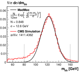
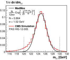
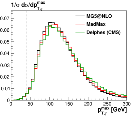
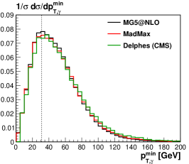
To simulate the detector effects in MadMax we modify MadGraph5 madgraph5 to smear the Higgs propagator like the square root of a Gaussian distribution. This allows us to reproduce the measured smearing of the CMS detector for Vernieri:2014wfa and pairs CMS:2016zjv . In the upper panels of Fig. 2 we show that our prescription is adequate for the peak region, but faces limitations for the tails of the invariant mass distributions. However, these tails will hardly contribute to the signal significance. All we need to do is account for the loss of signal rate through these tails, for the peak and for the peak.
Our choice of trigger cuts is motivated by CMS cms : GeV, GeV, , , GeV, GeV, , and GeV. Our invariant mass windows GeV and GeV are designed to fully contain the peaks, as illustrated in the first two panels of Fig. 2. We apply these mass windows for the continuum background simulation throughout or analysis, which means that our background kinematics will not fully reproduce the QCD features.
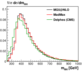
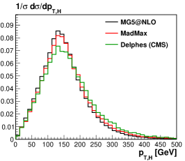
Also in Fig. 2 we show the distribution and the different transverse momentum spectra entering our analysis. The MadMax model is based on a a loop-improved approach hh_madgraph which includes the NLO form factors presented in Ref. spirix . This model is also used by the ATLAS collaboration atlas . One reference curve shows the full loop calculation using MG5-aMC@NLO nlo_madgraph , another a fast detector simulation with Delphes delphes . Even though our simulation might not correspond to a precision prediction at the per-cent level, we see that it reproduces the next-to-leading order results well.
II Standard Model signal vs. background
The first question we want to address in this study is: which kinematic features allow us to extract Higgs pair production from backgrounds? In this section we identify the Higgs self-coupling with its Standard Model value , ensuring the perfect threshold cancellation in the heavy top limit shown in Eq.(2). In our statistics language the null-hypothesis is continuum backgrounds only, while the hypothesis is defined by Standard Model signal plus backgrounds.
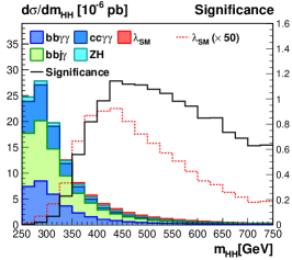
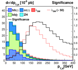
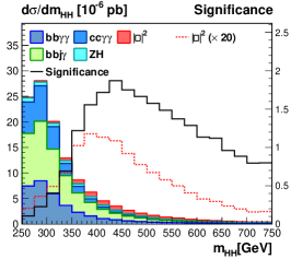
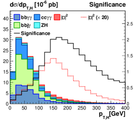
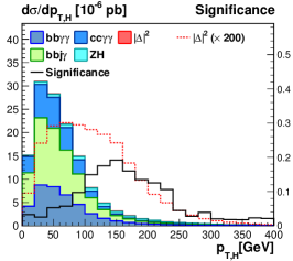
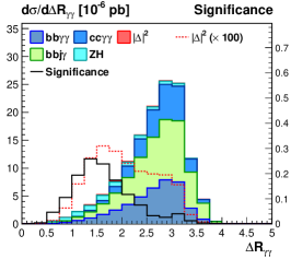
In Fig. 3 we show a set of kinematic distributions for the Higgs decay products and for the reconstructed Higgs. At the level we know that two distributions we want to study are the invariant mass distribution and the transverse momentum of each of the two reconstructed Higgses. The dashed red line simply scales the signal histogram so we can actually see its kinematic distribution. For both Higgs distributions the continuum backgrounds are considerably softer than the Higgs pair signal. The same is true for the transverse momenta of the Higgs decay products. From these distributions it is also clear that an upper bound on will help us extract the Higgs pair signal uli3 .
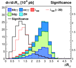
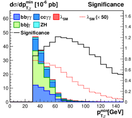
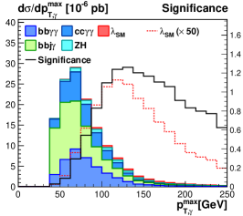
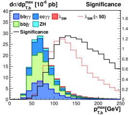
For the maximum significance with which we can extract the Standard Model signal from the continuum background we find a Gaussian equivalent of
| (10) |
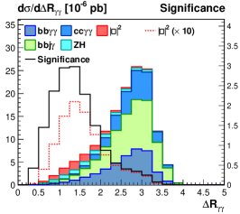
The black lines in Fig. 3 show how this significance is distributed over phase space. First, we observe that the threshold region GeV hardly contributes to the SM signal extraction. Instead, it seems crucial to include reconstructed Higgses with GeV, i.e. well in the boosted regime boosted ; madmax2 . The separation of the significance distribution from the signal distributions occurs because of the rapidly falling background distributions. Due to the Higgs boost, widely separated photons with will not help with the signal extraction, while in particular for the harder of the two photons or bottoms we can completely ignore the soft part of the spectrum.
One key question for any multi-variate analysis is if the phase space regions which dominate the signal vs background separation will be safe with respect to systematic and theoretical uncertainties. From the transverse momentum spectra in Fig. 3 we see that soft photons with GeV play hardly any role in separating the Higgs pair signal from the continuum background. Similarly, for the tagged bottom jets the relevant range is GeV. In this range we do not expect jet radiation and the related combinatorics to have a large effect on our results; the size of the usual perturbative rate corrections for the signal and background process should be theoretically under control. Finally, the relevant di-photon phase space is , clearly not a challenge for example to photon separation. A multi-variate analysis of Higgs pair production in the Standard Model should be straightforward.
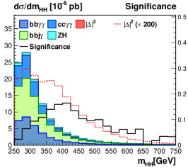
From Eq.(2) we know that the two Feynman diagrams contributing to Higgs pair production have distinct kinematic features, and their combination should allow us to understand the signal and significance distributions. In the upper panels of Fig. 4 we illustrate some of the kinematic distributions shown in Fig. 3, but for continuum Higgs pair production only. As expected, the two cases are similar, because the continuum diagram is responsible for almost the entire signal rate in the Standard Model. In the second set of plots we show the kinematic distributions of the triangle diagram only, i.e. the term of the cross section which carries the information on the Higgs self-coupling. As a first piece of information, we see that the significance with which we can extract the triangle diagrams in the absence of an interference with the continuum is extremely small. Kinematically, both in and this diagram has a considerably softer behavior. The two photons arising from a softer Higgs decay can now be more widely separated. These are the phase space regions where we can expect our signal vs background analysis to gain sensitivity to the value of the Higgs self-coupling, typically through an enhanced cancellation between the two Feynman diagrams shown in Fig. 1.
III Higgs self-coupling
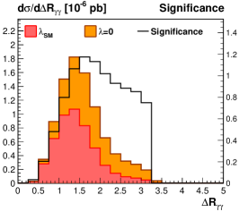
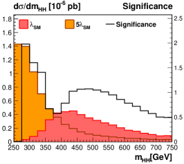
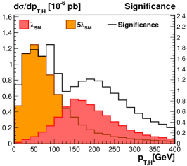
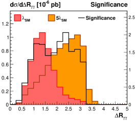
In the second part of the paper we investigate the question: what are the prospects of measuring the Higgs self-coupling in the presence of backgrounds? In Fig. 5 we show some kinematic distributions comparing two signal hypotheses, assuming a variable self-coupling
| (11) |
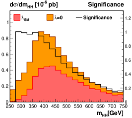
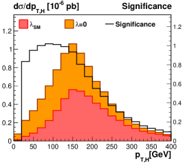
In the absence of a Higgs self-coupling we see that the Higgs pair production rate is significantly enhanced. While it is not immediately obvious from the two signal curves, the significance distribution over confirms that we can observe the effect of a zero self-coupling mostly close to threshold and for GeV. Similarly, the absence of a self-coupling will modify the transverse Higgs momentum around GeV. In the photon separation the sensitive range requires widely separated photons. We skip a detailed analysis of a slightly enhanced self-coupling , because it will be most visible through a significant reduction of the production rate. The dramatic case of is shown in the lower panels of Fig. 5. The kinematic distributions are now modified close to threshold and for small transverse momenta of each Higgs, as expected from an -channel-mediated process .
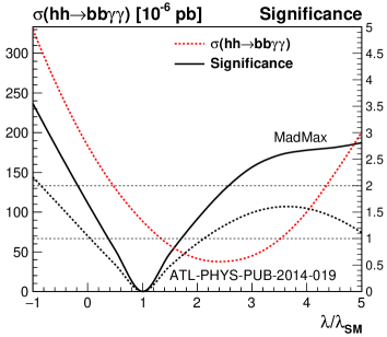
In the next step we add the QCD continuum and backgrounds and test how well we can extract the Higgs self-coupling from the kinematic information. In Fig. 6 we show the maximum significance of a multi-variate analysis as well as the significance from a counting experiment based on the total Higgs pair cross section after applying some basic cuts ATL-PHYS-PUB-2014-019 . As mentioned above, the Higgs pair production rate increases towards vanishing self-coupling, has a minimum of roughly a quarter of the Standard Model rate around , and increases again for larger self-couplings. The arguably most interesting case of zero self-coupling, related to a Higgs potential without the usual minimum, should be most easily distinguishable from the Standard Model spirix ; uli1 . The LHC will at best constrain the Higgs self-coupling range to be
| (12) |
and rule out
| (13) |
Obviously, we can try to combine this result with additional signatures to enhance the final reach of the LHC uli1 ; uli2 ; uli3 ; boosted .
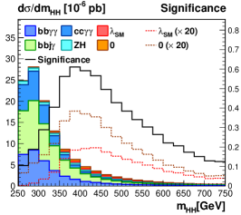
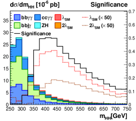
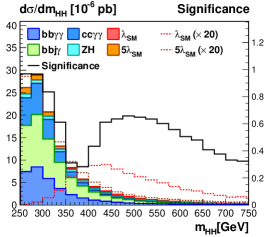
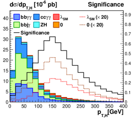
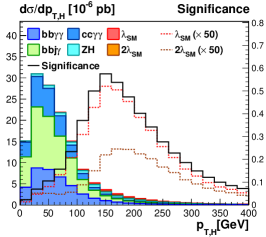
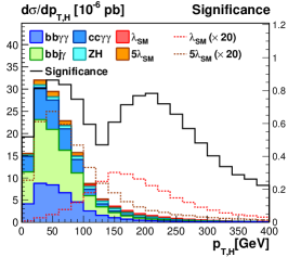
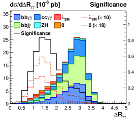
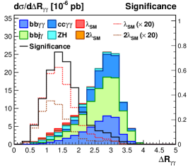
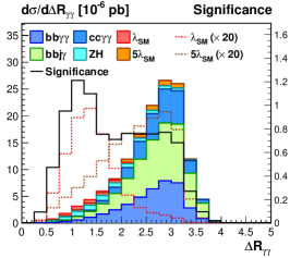
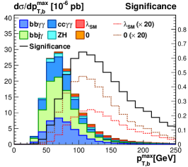
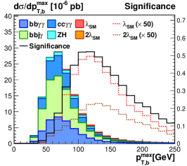
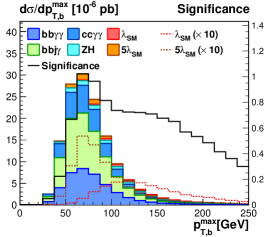
From all we have discussed to here, the obvious question is how much of the pure signal interference structure and its sensitivity to the self-coupling survives in the presence of backgrounds, and to what degree background uncertainties can mimic an anomalous self-coupling. In Fig. 7 we compare pairs of hypotheses for signal plus background, i.e. we test how well we can measure the Higgs self-coupling in the presence of the backgrounds. The Standard Model signal is shown in red and the alternative model with its shifted self-coupling is shown in orange. In our simulation we always apply mass windows for the and pairs, which already biases our background simulations towards signal-like, hard configurations. Nevertheless, in Fig. 7 we see that even then the QCD backgrounds still populate low- and low- regions. As already shown in Fig. 5, these are exactly the phase space regions where the sensitivity to an anomalous self-coupling is the largest.
For the measurement of in the presence of backgrounds, the sensitive regions of phase space are defined by a combination of background rejection and sensitivity to . While for background rejection described in Fig. 3 the region with high GeV and GeV are most useful, the self-coupling measurement requires lower- and lower- bins, as seen in Fig. 5. As a result, the significance peak in the SM background rejection around GeV moves to slightly below 400 GeV when we are interested in . Similarly, the background-driven significance at GeV and the self-coupling-sensitive region GeV together give a distinct peak at 150 GeV for or . In contrast, for a very large self-coupling the significance receives contributions from two distinct regions of phase space, GeV and GeV. The geometric separation of the two photons and the transverse momentum of the harder -jet follow the same pattern. This means that the most significant phase space regions for a measurement of the self-coupling are driven by the background rejection, shifted by the well-known regions of phase space carrying sensitivity to the self-coupling. Large deviations from the phase space regions for background rejection only occur when we test very large self-couplings.
IV Outlook
Multi-variate analyses often challenge our understanding of what limiting factors of important measurements are. To gauge the sensitivity for example of a Higgs self-coupling measurement to different sources of uncertainties we need to understand where the relevant phase space regions for a given measurement are madmax1 ; madmax2 .
In this paper we have studied the phase space regions which contribute to the extraction of the Higgs pair production signal from the continuum backgrounds, as well as those regions allowing for a measurement of the Higgs self-coupling. We focus on the signature uli3 , but expect our results to also hold for other channels with large continuum backgrounds. The two relevant phase space regions for the signal extraction and the coupling measurement are separate and in particular for the signal extraction well understood in terms of systematic and theoretical errors.
The most sensitive phase space region for extracting the self-coupling is close to threshold, where we expect the QCD background to overwhelm the Higgs pair signal. The main question will be how well we understand those backgrounds and how much of this region can still be used for the self-coupling measurement. Assuming SM-like self-coupling, the bulk of the coupling-sensitive region in the presence of QCD backgrounds is only slightly softer than the relevant phase space for the extraction of the Standard Model signal. For large self-couplings this region shifts significantly, forcing us to consider a proper hypothesis test for a variable Higgs self-coupling.
Acknowledgments
First, we still remember to Uli Baur for coming up with this measurement and for developing the first and original analyses. Second, we are grateful to Kyle Cranmer for his continuous support and to Bill Murray for his valuable comments concerning v1. Moreover, we would like to thank Martin Jankowiak for his contributions during an early phase of the project. We thank David Bourne and Anthony Yeates for helpful discussion. TP and PS would like to thank the MITP for the hospitality and support while this paper was finally written. The work of F.K. was supported by US Department of Energy under Grant DE-FG02-04ER-41298. F.K. also acknowledges support from the Fermilab Graduate Student Research Program in Theoretical Physics operated by Fermi Research Alliance, LLC under Contract No. DE-AC02-07CH11359 with the United States Department of Energy. P.S. work was supported in part by the European Union as part of the FP7 Marie Curie Initial Training Network MCnetITN (PITN-GA-2012-315877).
Appendix A Future 100 TeV Collider
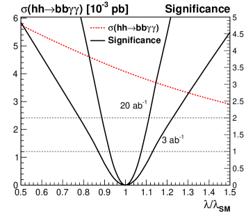
We can use exactly the same setup as in the main body of the paper to estimate the impact of the signal kinematics at a future 100 TeV collider with an integrated luminosity of . Several studies, largely based on a rate measurement with some background rejection cuts, have shown that Higgs pair production can be probed at such a machine with high precision Contino:2016spe ; nimatron_hh .
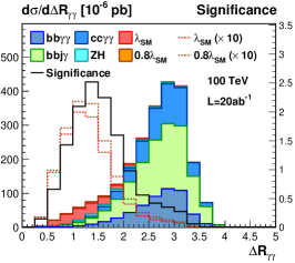
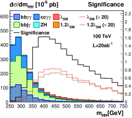
In Fig. 8 we show the maximum significance for distinguishing a modified Higgs self-coupling from the Standard Model at a future 100 TeV collider. The setup is exactly the same as for our LHC analysis leading to the results shown in Fig. 9. This includes our detector smearing as well as the trigger cuts. The signal cross section is now taken from MadMax without an external normalization. Relying on a multi-variate analysis we can at best constrain the Higgs self-coupling range to be
| (14) |
and rule out
| (15) |
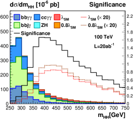
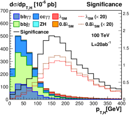
In Fig. 9 we also show the significance distribution over phase space. It is essentially identical to the 14 TeV case, because the relevant energy scale is given by the Standard Model Higgs mass in the two propagators. As for the LHC this implies that systematic and theoretical uncertainties should not pose a major issue for this precision measurement, which is driven by a very large number of signal events.
These 100 TeV results quoted above appear, at first, to disagree with some results shown in the literature. The main reason for this are diverging assumptions about tagging efficiencies. Since the Higgs decay products are mostly concentrated in the central detector, we do not expect the forward coverage of 100 TeV collider to significantly affect our results. However, we find that assumptions about -tagging are crucial. The signal’s -distribution peaks around and therefore in a regime with suppressed tagging efficiency, about 45% according to the parameterization in App. B. An improved -tagging efficiency at low transverse momentum will significantly enhance the signal rate and therefore improve the sensitivity for the triple-Higgs coupling. This explains the better reach quoted in in Ref. Contino:2016spe , which assumes a constant 75% tagging efficiency.


Appendix B Tagging efficiencies
Because the tagging and identification efficiencies have a crucial effect on our results, we give the necessary details in this Appendix. The -tagging efficiency and the corresponding mistag rate depends on the parton forming the tagged jet, the barrel respectively end-cap position in the detector, and the transverse momentum. The -related tagging efficiencies we use in our analysis are
| -jets | (18) | |||
| -jets | (21) | |||
| light-flavor jets | (22) |
For the photons we follow Ref. Butler:2020886 (Fig. 9.22), which suggests a photon identification efficiency and a -dependent mistag rate between and for jets between 50 GeV and 100 GeV:
| photon | ||||
| light-flavor jets | (25) |
References
- (1) O. J. P. Eboli, G. C. Marques, S. F. Novaes and A. A. Natale, Phys. Lett. B 197, 269 (1987); D. A. Dicus, C. Kao and S. S. D. Willenbrock, Phys. Lett. B 203, 457 (1988); E. W. N. Glover and J. J. van der Bij, Nucl. Phys. B 309, 282 (1988).
- (2) T. Plehn, M. Spira and P. M. Zerwas, Nucl. Phys. B 479, 46 (1996) Erratum: [Nucl. Phys. B 531, 655 (1998)]; A. Djouadi, W. Kilian, M. Muhlleitner and P. M. Zerwas, Eur. Phys. J. C 10, 45 (1999); X. Li and M. B. Voloshin, Phys. Rev. D 89, no. 1, 013012 (2014).
- (3) U. Baur, T. Plehn and D. L. Rainwater, Phys. Rev. Lett. 89, 151801 (2002); U. Baur, T. Plehn and D. L. Rainwater, Phys. Rev. D 67, 033003 (2003).
- (4) U. Baur, T. Plehn and D. L. Rainwater, Phys. Rev. D 68, 033001 (2003).
- (5) U. Baur, T. Plehn and D. L. Rainwater, Phys. Rev. D 69, 053004 (2004).
- (6) J. Baglio, A. Djouadi, R. Gröber, M. M. Mühlleitner, J. Quevillon and M. Spira, JHEP 1304, 151 (2013).
- (7) for a currrent analysis see e.g. T. Corbett, O. J. P. Eboli, D. Goncalves, J. Gonzalez-Fraile, T. Plehn and M. Rauch, JHEP 1508, 156 (2015).
- (8) M. L. Mangano, T. Plehn, P. Reimitz, T. Schell and H. S. Shao, J. Phys. G 43, no. 3, 035001 (2016).
- (9) for an up-to-date analysis of the Higgs-gauge sector see A. Butter, O. J. P. Eboli, J. Gonzalez-Fraile, M. C. Gonzalez-Garcia, T. Plehn and M. Rauch, arXiv:1604.03105 [hep-ph].
- (10) F. Goertz, A. Papaefstathiou, L. L. Yang and J. Zurita, JHEP 1504, 167 (2015); Q. H. Cao, B. Yan, D. M. Zhang and H. Zhang, Phys. Lett. B 752, 285 (2016); M. Gorbahn and U. Haisch, arXiv:1607.03773 [hep-ph]; G. Degrassi, P. P. Giardino, F. Maltoni and D. Pagani, arXiv:1607.04251 [hep-ph].
- (11) M. A. Shifman, A. I. Vainshtein, M. B. Voloshin and V. I. Zakharov, Sov. J. Nucl. Phys. 30, 711 (1979) [Yad. Fiz. 30, 1368 (1979)]. B. A. Kniehl and M. Spira, Z. Phys. C 69, 77 (1995); M. Spira, arXiv:1607.05548 [hep-ph].
- (12) M. J. Dolan, C. Englert and M. Spannowsky, JHEP 1210, 112 (2012); A. J. Barr, M. J. Dolan, C. Englert and M. Spannowsky, Phys. Lett. B 728, 308 (2014).
- (13) V. Barger, L. L. Everett, C. B. Jackson, A. D. Peterson and G. Shaughnessy, Phys. Rev. D 90, no. 9, 095006 (2014).
- (14) G. Aad et al. [ATLAS Collaboration], Phys. Rev. D 92, 092004 (2015).
- (15) V. Khachatryan et al. [CMS Collaboration], arXiv:1603.06896 [hep-ex].
- (16) A. Papaefstathiou, L. L. Yang and J. Zurita, Phys. Rev. D 87, no. 1, 011301 (2013).
- (17) D. E. Ferreira de Lima, A. Papaefstathiou and M. Spannowsky, JHEP 1408, 030 (2014); D. Wardrope, E. Jansen, N. Konstantinidis, B. Cooper, R. Falla and N. Norjoharuddeen, Eur. Phys. J. C 75, no. 5, 219 (2015); J. K. Behr, D. Bortoletto, J. A. Frost, N. P. Hartland, C. Issever and J. Rojo, Eur. Phys. J. C 76, no. 7, 386 (2016).
- (18) Q. Li, Z. Li, Q. S. Yan and X. Zhao, Phys. Rev. D 92, no. 1, 014015 (2015).
- (19) see e.g. J. M. No and M. Ramsey-Musolf, Phys. Rev. D 89, no. 9, 095031 (2014); B. Hespel, D. Lopez-Val and E. Vryonidou, JHEP 1409, 124 (2014); C. Y. Chen, S. Dawson and I. M. Lewis, Phys. Rev. D 91, no. 3, 035015 (2015); P. Huang, A. Joglekar, B. Li and C. E. M. Wagner, Phys. Rev. D 93, no. 5, 055049 (2016).
- (20) R. Gröber and M. Mühlleitner, JHEP 1106, 020 (2011); R. Gröber, M. Mühlleitner and M. Spira, JHEP 1606, 080 (2016).
- (21) S. Dawson, S. Dittmaier and M. Spira, Phys. Rev. D 58, 115012 (1998); J. Grigo, J. Hoff, K. Melnikov and M. Steinhauser, Nucl. Phys. B 875, 1 (2013); F. Maltoni, E. Vryonidou and M. Zaro, JHEP 1411, 079 (2014).
- (22) D. de Florian and J. Mazzitelli, JHEP 1509, 053 (2015); J. Grigo, J. Hoff and M. Steinhauser, Nucl. Phys. B 900, 412 (2015)l S. Borowka, N. Greiner, G. Heinrich, S. P. Jones, M. Kerner, J. Schlenk, U. Schubert and T. Zirke, Phys. Rev. Lett. 117, no. 1, 012001 (2016); D. de Florian, M. Grazzini, C. Hanga, S. Kallweit, J. M. Lindert, P. Maierhofer, J. Mazzitelli and D. Rathlev, arXiv:1606.09519 [hep-ph].
- (23) K. Cranmer and T. Plehn, Eur. Phys. J. C 51, 415 (2007).
- (24) T. Plehn, P. Schichtel and D. Wiegand, Phys. Rev. D 89, no. 5, 054002 (2014).
- (25) for a proof and corresponding definitions, see e.g. J. Stuart, A. Ord and S. Arnold, Kendall’s Advanced Theory of Statistics, Vol 2A (6th Ed.) (Oxford University Press, New York, 1994); for a pedagogical introduction in the context of high-energy physics, see A. Read, in ‘1st Workshop on Confidence Limits’, CERN Report No. CERN-2000-005 (2000).
- (26) Lloyd N. Trefethen, Spectral Methods in MATLAB (2000), ISBN: 978-0-89871-465-4.
- (27) K. Cranmer, LEPStats4LHC, http://phystat.org/phystat/packages/0703002.1.html
- (28) C. Vernieri [CMS Collaboration], arXiv:1411.4362 [hep-ex].
- (29) CMS Collaboration [CMS Collaboration], CMS-PAS-HIG-15-005.
- (30) R. Frederix, S. Frixione, V. Hirschi, F. Maltoni, O. Mattelaer, P. Torrielli, E. Vryonidou and M. Zaro, Phys. Lett. B 732, 142 (2014).
- (31) J. de Favereau et al. [DELPHES 3 Collaboration], JHEP 1402, 057 (2014).
- (32) P. Eller, arXiv:1408.5044 [hep-ex].
- (33) J. Anderson et al., arXiv:1309.1057 [hep-ex].
- (34) J. Butler, D. Contardo, M. Klute, J. Mans, and L. Silvestris, CERN-LHCC-2015-010.
- (35) J. Alwall, M. Herquet, F. Maltoni, O. Mattelaer and T. Stelzer, JHEP 1106, 128 (2011).
- (36) J. Alwall et al., JHEP 1407, 079 (2014).
- (37) ATLAS Collaboration [ATLAS Collaboration], ATL-PHYS-PUB-2014-019.
- (38) A. J. Barr, M. J. Dolan, C. Englert, D. E. Ferreira de Lima and M. Spannowsky, JHEP 1502, 016 (2015); A. Azatov, R. Contino, G. Panico and M. Son, Phys. Rev. D 92, no. 3, 035001 (2015); A. Papaefstathiou, Phys. Rev. D 91, no. 11, 113016 (2015); H. J. He, J. Ren and W. Yao, Phys. Rev. D 93, no. 1, 015003 (2016); A. Papaefstathiou and K. Sakurai, JHEP 1602, 006 (2016); C. Y. Chen, Q. S. Yan, X. Zhao, Y. M. Zhong and Z. Zhao, Phys. Rev. D 93, no. 1, 013007 (2016); B. Fuks, J. H. Kim and S. J. Lee, Phys. Rev. D 93, no. 3, 035026 (2016).
- (39) R. Contino et al., arXiv:1606.09408 [hep-ph].