An exponential B-spline collocation method for fractional sub-diffusion equation

Abstract

In this article, we propose an exponential B-spline collocation method to approximate the solution of the fractional sub-diffusion equation of Caputo type. The present method is generated by use of the Gorenflo-Mainardi-Moretti-Paradisi (GMMP) scheme in time and an efficient exponential B-spline based method in space. The unique solvability is rigorously discussed. Its stability is well illustrated via a procedure closely resembling the classic von Neumann approach. The resulting algebraic system is tri-diagonal that can rapidly be solved by the known algebraic solver with low cost and storage. A series of numerical examples are finally carried out and by contrast to the other algorithms available in the literature, numerical results confirm the validity and superiority of our method.

1 Introduction

The basic concept of anomalous diffusion dates back to Richardson’s treatise on atmospheric diffusion in 1926 [31]. It has increasingly got recognition since the late 1960s within transport theory. In contrast to a typical diffusion, such process no longer follows Gaussian statistics, then the classic Fick’s law fails to apply. Its most striking character is the temporal power-law pattern dependence of the mean squared displacement [22], i.e., $\chi^{2}(t)\sim\kappa t^{\alpha}$, for sub-diffusion, $\alpha<1$, while $\alpha>1$ for super-diffusion. Anomalous transport behavior is ubiquitous in physical scenarios and due to its universal mutuality, formidable challenges are introduced. In recent decades, fractional partial differential equations (PDEs) enter public vision that compare favorably with the usual models to characterize such transport motions in heterogeneous aquifer and the medium with fractal geometry [1, 26]. An explosive interest has been gained among academic circles to scramble to investigate the theoretical properties, analytic techniques, and numerical algorithms for fractional PDEs [2, 5, 7, 18, 21, 23, 29, 36].

As a model problem of the class of fractional PDEs described above, the fractional sub-diffusion equation is considered here

$$\frac{\partial^{\alpha}u(x,t)}{\partial t^{\alpha}}-\kappa\frac{\partial^{2}u(x,t)}{\partial x^{2}}=f(x,t),\quad a<x<b,\ 0<t\leq T,$$ (1.1)

subjected to the initial and boundary conditions as

$$u(x,0)=\varphi(x),\quad a\leq x\leq b,$$ (1.2)

$$u(a,t)=g_{1}(t),\quad u(b,t)=g_{2}(t),\quad 0<t\leq T,$$ (1.3)

where $0<\alpha<1$, $\kappa$ is the positive viscosity constant, and $\varphi(x)$, $g_{1}(t)$, $g_{2}(t)$ are the prescribed functions with sufficient smoothness. In Eq. (1.1), the time-fractional derivative is defined in Caputo sense, i.e.,

$$\frac{\partial^{\alpha}u(x,t)}{\partial t^{\alpha}}=\frac{1}{\Gamma(1-\alpha)}\int^{t}_{0}\frac{\partial u(x,\xi)}{\partial\xi}\frac{d\xi}{(t-\xi)^{\alpha}},$$

with the Gamma function $\Gamma(\cdot)$. There have already been some works dedicated to develop numerical algorithms to solve Eqs. (1.1)-(1.3) apart from a few analytic methods that are not always available for general situations. Zhang and Liu derived an implicit difference scheme and proved that it is unconditional stable [37]. Yuste and Acedo studied an explicit difference scheme based on Grünwald-Letnikov formula [34]. Along the same line, a group of weighted average difference schemes was then obtained [33]. In [4], Cui raised a high-order compact difference scheme and its convergence was detailedly discussed; another similar approach was the compact scheme stated in [30], for the fractional sub-diffusion equation with Neumann boundary condition. In [15], an effective spectral method was constructed by using the common $L^{1}$-formula in time and a Legendre spectral approximation in space. Later, this method was extended to the time-space case [14]. The finite element method was considered by Jiang and Ma [10]. The semi-discrete lump finite element method was studied by Jin et al. for a time-fractional model with a nonsmooth right-hand side [11]. Liu et al. described an implicit RBF meshless approach for the time-fractional diffusion equation [16]. Li et al. suggested an adomian decomposition algorithm for the equations of the same type [13]. In [9], the authors solved such a model by the direct discontinuous Galerkin method with the Caputo derivative discretized by a GMMP scheme. Recently, Luo et al. established a quadratic spline collocation method for the fractional sub-diffusion equation [17], where the convergence under $L^{\infty}$-norm was analyzed. Sayevand et al. conducted a cubic B-spline collocation method [32], whose stability was provided as well. In [27], a Sinc-Haar collocation method was proposed, which used the Haar operational matrix to convert the original problem into linear algebraic equations.

In the present work, regarding the current interest in efficient numerical algorithms for fractional PDEs, we showcase a collocation method based on exponential B-spline trial function to solve Eqs. (1.1)-(1.3). The Caputo derivative is tackled by GMMP formula and the spatial derivative is approximated in an exponential spline space via a uniform nodal collocation strategy. A von Neumann like procedure leads to its unconditional stability. Its codes are tested on five numerical examples and studied in contrast with the other algorithms. The obtained method is highly accurate and calls for a lower cost to implement. This may make sense to treat the equations as the model we consider here with a long time range. The outline is as follows. In Section 2, we give a concise description of the exponential B-spline trial basis, which will be useful hereinafter. In Section 3, we construct a fully discrete exponential B-spline method on uniform meshes to discretize the model and prove that it is stable. The initial vector is addressed in Section 4, which we require to start our method. To evaluate its accuracy and advantages, numerical examples are covered in Section 5.

2 Description of exponential spline functions

In the sequel, let $a=x_{0}<x_{1}<x_{2}<\cdots<x_{M-1}<x_{M}=b$ be an equidistant spatial mesh on the interval $[a,b]$, and for $M\in\mathbb{N}^{+}$, denote

$$h=(b-a)/M,\quad p=\max\limits_{1\leq j\leq M}p_{j},\quad s=\sinh(ph),\quad c=\cosh(ph),$$

where $p_{j}$ is the value of function $p(x)$ at mesh knot $x_{j}$. The exponential splines are a kind of piecewise non-polynomial functions that are known as a generalization of the semi-classical cubic splines. They are recognized as a continuum of interpolants ranging from the cubic splines to the linear cases [19]. Also, like the polynomial splines, a basis of exponential B-splines is admitted and an advisable definition is the one introduced by McCartin [20], each of which is support on finite subsegments. On the above mesh together with another six knots $x_{j}$, $j=-3,-2,-1,M+1,M+2,M+3$ beyond $[a,b]$, the mentioned exponential B-splines $B_{j}(x)$, $j=-1,0,\ldots,M+1$, are given as follows

$$B_{j}(x)=\left\{\begin{aligned} &e(x_{j-2}-x)-\frac{e}{p}\sinh(p(x_{j-2}-x)),\,\qquad\quad\qquad\qquad\qquad\textrm{if}\ \ x\in[x_{j-2},x_{j-1}],\\ &a+b(x_{j}-x)+c\exp(p(x_{j}-x))+d\exp(-p(x_{j}-x)),\quad\textrm{if}\ \ x\in[x_{j-1},x_{j}],\\ &a+b(x-x_{j})+c\exp(p(x-x_{j}))+d\exp(-p(x-x_{j})),\quad\textrm{if}\ \ x\in[x_{j},x_{j+1}],\\ &e(x-x_{j+2})-\frac{e}{p}\sinh(p(x-x_{j+2})),\,\qquad\quad\qquad\qquad\qquad\textrm{if}\ \ x\in[x_{j+1},x_{j+2}],\\ &0,\quad\textrm{otherwise},\end{aligned}\right.$$

where

$$e=\frac{p}{2(phc-s)},\quad a=\frac{phc}{phc-s},\quad b=\frac{p}{2}\bigg{[}\frac{c(c-1)+s^{2}}{(phc-s)(1-c)}\bigg{]},$$

$$c=\frac{1}{4}\bigg{[}\frac{\exp(-ph)(1-c)+s(\exp(-ph)-1)}{(phc-s)(1-c)}\bigg{]},\quad d=\frac{1}{4}\bigg{[}\frac{\exp(ph)(c-1)+s(\exp(ph)-1)}{(phc-s)(1-c)}\bigg{]}.$$

The values of $B_{j}(x)$ at each knot are given as

$$B_{j}(x_{k})=\left\{\begin{aligned} &1,&\textrm{if}\ \ k=j,\\ &\frac{s-ph}{2(phc-s)},&\textrm{if}\ \ k=j\pm 1,\\ &0,&\textrm{if}\ \ k=j\pm 2.\end{aligned}\right.$$ (2.4)

The values of $B^{\prime}_{j}(x)$ and $B^{\prime\prime}_{j}(x)$ at each knot are given as

$$B^{\prime}_{j}(x_{k})=\left\{\begin{aligned} &0&\textrm{if}\ \ k=j,\\ &\frac{\mp p(1-c)}{2(phc-s)},&\textrm{if}\ \ k=j\pm 1,\\ &0,&\textrm{if}\ \ k=j\pm 2,\end{aligned}\right.$$ (2.5)

and

$$B^{\prime\prime}_{j}(x_{k})=\left\{\begin{aligned} &\frac{-p^{2}s}{phc-s},&\textrm{if}\ \ k=j,\\ &\frac{p^{2}s}{2(phc-s)},&\textrm{if}\ \ k=j\pm 1,\\ &0,&\textrm{if}\ \ k=j\pm 2.\end{aligned}\right.$$ (2.6)

The set of $B_{j}(x)\in C^{2}(\mathbb{R})$, $j=-1,0,\ldots,M+1$, are linearly independent and form an exponential spline space on $[a,b]$. The non-negative free $p$ is termed “tension” parameter and $p\rightarrow 0$ yields cubic spline whereas $p\rightarrow\infty$ corresponds to the linear spline. The cubic spline interpolation causes extraneous inflexion points while the exponential spline interpolation allows to remedy this issue.

3 An exponential B-spline collocation method

Let $t_{n}=n\tau$, $n=0,1,\ldots,N$, $T=\tau N$, $N\in\mathbb{N}^{+}$, and $x_{j}=a+jh$, $j=-1,0,\ldots,M+1$, $h=(b-a)/M$, $M\in\mathbb{N}^{+}$. On the time-space lattice, we set about deriving the exponential B-spline collocation method for Eqs. (1.1)-(1.3).

3.1 GMMP scheme for Caputo derivative

To start with, we recall the Caputo and Riemann-Liouville fractional derivatives. Given a smooth enough $f(x,t)$, the $\alpha$-th Caputo derivative is defined by

$${{}^{C}_{0}}D^{\alpha}_{t}f(x,t)=\frac{1}{\Gamma(m-\alpha)}\int^{t}_{0}\frac{\partial^{m}f(x,\xi)}{\partial\xi^{m}}\frac{d\xi}{(t-\xi)^{1+\alpha-m}},$$ (3.7)

and the $\alpha$-th Riemann-Liouville type derivative is defined by

$${{}^{RL}_{0}}D^{\alpha}_{t}f(x,t)=\frac{1}{\Gamma(m-\alpha)}\frac{\partial^{m}}{\partial t^{m}}\int^{t}_{0}\frac{f(x,\xi)d\xi}{(t-\xi)^{1+\alpha-m}},$$ (3.8)

where, $m-1<\alpha<m$, $m\in\mathbb{N}$ is not less than $1$. In common sense, (3.7) owns merits in handling the initial-valued problems, and thereby is utilized in time in most instances. (3.7), (3.8) interconvert into each other through

$${{}^{C}_{0}}D^{\alpha}_{t}f(x,t)={{}^{RL}_{0}}D^{\alpha}_{t}f(x,t)-\sum^{m-1}_{l=0}\frac{f^{(l)}(x,0)t^{l-\alpha}}{\Gamma(l+1-\alpha)}.$$ (3.9)

They are equal when $f^{(k)}(x,0)=0$, $k=0,1,\ldots,m-1$ are fixed; we refer the readers to [12, 28] for deeper insight. A GMMP scheme is derived by rewriting Eq. (3.9) and using a proper scheme to discretize (3.8), which reads [24]

$${{}^{C}_{0}}D^{\alpha}_{t}f(x,t_{n})\approx\frac{1}{\tau^{\alpha}}\sum_{k=0}^{n}\omega^{\alpha}_{k}f(x,t_{n-k})-\frac{1}{\tau^{\alpha}}\sum^{m-1}_{l=0}\sum^{n}_{k=0}\frac{\omega^{\alpha}_{k}f^{(l)}(x,0)t_{n-k}^{l}}{l!},$$ (3.10)

with several valid sets of coefficients $\omega^{\alpha}_{k}$ [34]. In particular, when

$$\omega^{\alpha}_{k}=(-1)^{k}\binom{\alpha}{k}=\frac{\Gamma{(k-\alpha)}}{\Gamma{(-\alpha)}\Gamma{(k+1)}},\quad k=0,1,2,\ldots$$ (3.11)

it is the one given by Gorenflo et al. [8]. In what follows, we chiefly consider such case; on selecting $\omega^{\alpha}_{k}$ as (3.11) and imposing $0<\alpha<1$, (3.10) simply reduces to

$${{}^{C}_{0}}D^{\alpha}_{t}f(x,t_{n})=\frac{1}{\tau^{\alpha}}\sum_{k=0}^{n}\omega^{\alpha}_{k}f(x,t_{n-k})-\frac{1}{\tau^{\alpha}}\sum_{k=0}^{n}\omega^{\alpha}_{k}f(x,0)+\mathscr{R}_{\tau},$$ (3.12)

with the truncated error $\mathscr{R}_{\tau}$ satisfying $\mathscr{R}_{\tau}=\mathscr{O}(\tau)$.

Lemma 3.1.

The coefficients $\omega^{\alpha}_{k}$ defined in (3.11) fulfill

• $\omega^{\alpha}_{0}=1,\quad\omega^{\alpha}_{k}<0$,   $\forall k\geq 1$,

• $\sum_{k=0}^{\infty}\omega^{\alpha}_{k}=0,\quad\sum_{k=0}^{n-1}\omega^{\alpha}_{k}>0$.

Proof.

See references [6, 28] for details. ∎

3.2 A fully discrete exponential B-spline based scheme

Define $V_{M+3}=\textrm{span}\{B_{-1}(x),B_{0}(x),\ldots,B_{M}(x),B_{M+1}(x)\}$ over the interval $[a,b]$ referred to as a $(M+3)$-dimensional exponential spline space. Then, an approximate solution to Eqs. (1.1)-(1.3) is sought on $V_{M+3}$ in the form

$$u_{N}(x,t)=\sum_{j=-1}^{M+1}\alpha_{j}(t)B_{j}(x),$$ (3.13)

with the unknown weights $\{\alpha_{j}(t)\}_{j=-1}^{M+1}$ yet to be determined by some certain restrictions. Discretizing Eq. (1.1) by using (3.12) in time, we have

$$u(x,t_{n})-\tau^{\alpha}\kappa\frac{\partial^{2}u(x,t_{n})}{\partial x^{2}}=-\sum_{k=1}^{n-1}\omega^{\alpha}_{k}u(x,t_{n-k})+\sum_{k=0}^{n-1}\omega^{\alpha}_{k}u(x,0)+\tau^{\alpha}f(x,t_{n})+\tau^{\alpha}\mathscr{R}_{\tau}.$$

Let $\alpha^{n}_{j}=\alpha_{j}(t_{n})$. On replacing $u(x,t)$ by $u_{N}(x,t)$ and imposing the following collocation and boundary conditions

$$u_{N}(x_{j},t_{n})-\tau^{\alpha}\kappa\frac{\partial^{2}u_{N}(x_{j},t_{n})}{\partial x^{2}}=-\sum_{k=1}^{n-1}\omega^{\alpha}_{k}u_{N}(x_{j},t_{n-k})+\sum_{k=0}^{n-1}\omega^{\alpha}_{k}u_{N}(x_{j},0)+\tau^{\alpha}f(x_{j},t_{n}),$$

$$u_{N}(x_{0},t_{n})=g_{1}(t_{n}),\quad u_{N}(x_{M},t_{n})=g_{2}(t_{n}),$$

at each nodal point $x_{j}$, $j=0,1,\ldots,M$, we obtain

$$A\alpha^{n}_{j-1}+A^{\prime}\alpha^{n}_{j}+A\alpha^{n}_{j+1}=-\sum_{k=1}^{n-1}\omega^{\alpha}_{k}P^{n-k}_{j}+\sum_{k=0}^{n-1}\omega^{\alpha}_{k}P_{j}^{0}+R^{n}_{j},$$ (3.14)

and the boundary sets

$$\frac{s-ph}{2(phc-s)}\alpha^{n}_{-1}+\alpha^{n}_{0}+\frac{s-ph}{2(phc-s)}\alpha^{n}_{1}=g_{1}^{n},$$ (3.15)

$$\frac{s-ph}{2(phc-s)}\alpha^{n}_{M-1}+\alpha^{n}_{M}+\frac{s-ph}{2(phc-s)}\alpha^{n}_{M+1}=g_{2}^{n},$$ (3.16)

owing to (3.13) and (2.4)-(2.6), with

$$A=-\tau^{\alpha}\kappa p^{2}s+\omega^{\alpha}_{0}(s-ph),\quad A^{\prime}=2\tau^{\alpha}\kappa p^{2}s+2\omega^{\alpha}_{0}(phc-s),$$

$$P^{m}_{j}=(s-ph)\alpha^{m}_{j-1}+2(phc-s)\alpha^{m}_{j}+(s-ph)\alpha^{m}_{j+1},\quad R^{n}_{j}=2\tau^{\alpha}(phc-s)f_{j}^{n}.$$

where $m=0,1,\ldots,n-1$. As a result, using Eqs. (3.15)-(3.16) to remove the unknown variables $\alpha^{n}_{-1}$, $\alpha^{n}_{M+1}$ in Eq.(3.14) when $j=0$, $M$, the above system admits a linear system of algebraic equations of size $(M+1)\times(M+1)$, as below

$$\textbf{A}\boldsymbol{\alpha}^{n}=-\sum_{k=1}^{n-1}\omega^{\alpha}_{k}\textbf{B}\boldsymbol{\alpha}^{n-k}+\sum_{k=0}^{n-1}\omega^{\alpha}_{k}\textbf{B}\boldsymbol{\alpha}^{0}+\textbf{F}^{n},$$ (3.17)

where

$$\textbf{A}=\left(\begin{array}[]{ccccc}2\tau^{\alpha}\kappa p^{3}hs(c-1)&0&&&\\ A&A^{\prime}&A&&\\ &\cdots&\ldots&\ldots&\\ &&\ldots&\ldots&\ldots\\ &&A&A^{\prime}&A\\ &&&0&2\tau^{\alpha}\kappa p^{3}hs(c-1)\\ \end{array}\right),$$

$$\textbf{B}=\left(\begin{array}[]{ccccc}0&0&&&\\ s-ph&2(phc-s)&s-ph&&\\ &\cdots&\ldots&\ldots&\\ &&\ldots&\ldots&\ldots\\ &&s-ph&2(phc-s)&s-ph\\ &&&0&0\\ \end{array}\right),$$

$$\boldsymbol{\alpha}^{m}=\left(\begin{array}[]{c}\alpha^{m}_{0}\\ \alpha^{m}_{1}\\ \vdots\\ \alpha^{m}_{M-1}\\ \alpha^{m}_{M}\end{array}\right),\ \ \textbf{F}^{n}=(phc-s)\left(\begin{array}[]{c}2\tau^{\alpha}(s-ph)f^{n}_{0}+d^{n}_{0}\\ 2\tau^{\alpha}f^{n}_{1}\\ \vdots\\ 2\tau^{\alpha}f^{n}_{M-1}\\ 2\tau^{\alpha}(s-ph)f^{n}_{M}+d^{n}_{M}\end{array}\right),$$

in which, $m=0,1,\ldots,n$, and $d^{n}_{0}$, $d^{n}_{M}$ are as follows

$$d^{n}_{0}=-2(s-ph)\sum_{k=0}^{n-1}\omega^{\alpha}_{k}g_{1}^{n-k}+2(s-ph)\sum_{k=0}^{n-1}\omega^{\alpha}_{k}\varphi_{0}+2\tau^{\alpha}\kappa p^{2}sg^{n}_{1},$$

$$d^{n}_{M}=-2(s-ph)\sum_{k=0}^{n-1}\omega^{\alpha}_{k}g_{2}^{n-k}+2(s-ph)\sum_{k=0}^{n-1}\omega^{\alpha}_{k}\varphi_{M}+2\tau^{\alpha}\kappa p^{2}sg^{n}_{2}.$$

The weights $\boldsymbol{\alpha}^{n}$ depends on $\boldsymbol{\alpha}^{n-k}$, $k=0,1,\ldots,n$, at its previous time levels and is found via a recursive style; once $\boldsymbol{\alpha}^{n}$ is obtained, $\alpha^{n}_{-1}$, $\alpha^{n}_{M+1}$ are obvious due to Eqs. (3.15)-(3.16). On the other side, A is a $(M+1)\times(M+1)$ tri-diagonal matrix, therefore the system can be performed by the well-known Thomas algorithm, which simply needs the arithmetic operation cost $\mathscr{O}(M+1)$.

4 Initial state

In order to start Eq. (3.17), an appropriate initial vector $\boldsymbol{\alpha}^{0}$ to the system is required. To this end, we employ the initial conditions

$$u_{N}(x_{j},0)=\varphi(x_{j}),\quad j=0,1,\cdots,M,$$

together with the collocation constraints

$$u^{\prime}_{N}(x_{0},0)=\varphi^{\prime}(x_{0}),\quad\ u^{\prime}_{N}(x_{M},0)=\varphi^{\prime}(x_{M}),$$

got via Eq. (1.2) explicitly to determine a unique initial vector $\boldsymbol{\alpha}^{0}$ by

$$\textbf{K}\boldsymbol{\alpha}^{0}=\textbf{U},$$ (4.18)

with the notations

$$\textbf{K}=\left(\begin{array}[]{ccccc}phc-s&s-ph&&&\\ s-ph&2(phc-s)&s-ph&&\\ &\cdots&\ldots&\ldots&\\ &&\ldots&\ldots&\ldots\\ &&s-ph&2(phc-s)&s-ph\\ &&&s-ph&phc-s\\ \end{array}\right),$$

$$\boldsymbol{\alpha}^{0}=\left(\begin{array}[]{c}\alpha^{0}_{0}\\ \alpha^{0}_{1}\\ \vdots\\ \alpha^{0}_{M-1}\\ \alpha^{0}_{M}\end{array}\right),\ \quad\textbf{U}=(phc-s)\left(\begin{array}[]{c}\varphi_{0}-\frac{(s-ph)\varphi^{\prime}(x_{0})}{p(1-c)}\\ 2\varphi_{1}\\ \vdots\\ 2\varphi_{M-1}\\ \varphi_{M}+\frac{(s-ph)\varphi^{\prime}(x_{M})}{p(1-c)}\end{array}\right).$$

In the same fashion, K is a $(M+1)\times(M+1)$ tri-diagonal matrix, so the solution of Eq. (4.18) can also be computed by Thomas algorithm.

5 Stability and solvability

In this section, our objective is to prove that Eqs. (3.17)-(4.18) are uniquely solvable and unconditionally stable. If $\tilde{\alpha}^{n}_{j}$, $n\geq 1$, is a perturbed solution of Eq. (3.14), we shall study how the perturbation $\rho^{n}_{j}=\alpha^{n}_{j}-\tilde{\alpha}^{n}_{j}$, which solves the homogeneous counterpart of the equation by

$$A\rho^{n}_{j-1}+A^{\prime}\rho^{n}_{j}+A\rho^{n}_{j+1}=-\sum_{k=1}^{n-1}\omega^{\alpha}_{k}Z^{n-k}_{j}+\sum_{k=0}^{n-1}\omega^{\alpha}_{k}Z_{j}^{0},$$ (5.19)

evolves over time, where $Z^{0}_{j}$, $Z^{n-k}_{j}$ are the quantities like $P^{0}_{j}$, $P^{n-k}_{j}$ with regard to the perturbation. Since the classic von Neumann method does not work for Eq. (5.19), a fractional procedure is employed to analyze its stability. This extension was recently laid down in [35] applied to discuss a non-uniform implicit difference scheme for fractional diffusion equations.

Lemma 5.1.

The system (3.17)-(4.18) are uniquely solvable since their coefficient matrices A, K are strictly diagonally dominant.

Proof.

In virtue of $A$, $A^{\prime}$, one gets

$$\big{|}A^{\prime}\big{|}-2\big{|}A\big{|} =2\big{|}\tau^{\alpha}\kappa p^{2}s+\omega^{\alpha}_{0}(phc-s)\big{|}-2\big{|}-\tau^{\alpha}\kappa p^{2}s+\omega^{\alpha}_{0}(s-ph)\big{|}$$

$$\geq 2\omega^{\alpha}_{0}(phc-s)-2\omega^{\alpha}_{0}(s-ph),$$

$$=2\omega^{\alpha}_{0}\big{(}(phc-s)-(s-ph)\big{)}.$$

Then, the lemma is ascribed to $s-ph<phc-s$. Using the following Taylor’s expansions

$$s-ph=\frac{(ph)^{3}}{3!}+\frac{(ph)^{5}}{5!}+\cdots+\frac{(ph)^{2k+1}}{(2k+1)!}+\cdots$$

$$phc-ph=\frac{(ph)^{3}}{2!}+\frac{(ph)^{5}}{4!}+\cdots+\frac{(ph)^{2k+1}}{(2k)!}+\cdots$$

results in

$$(phc-ph)-2(s-ph) =(ph)^{3}\Bigg{(}\frac{1}{2!}-\frac{2}{3!}\Bigg{)}+(ph)^{5}\Bigg{(}\frac{1}{4!}-\frac{2}{5!}\Bigg{)}$$

$$\quad+\cdots+(ph)^{2k+1}\Bigg{(}\frac{1}{(2k)!}-\frac{2}{(2k+1)!}\Bigg{)}+\cdots$$

Due to $(2k)!\times 2<(2k)!\times(2k+1)$, $k\geq 1$, there exist

$$(phc-s)-(s-ph)=(phc-ph)-2(s-ph)>0,$$

and $\big{|}A^{\prime}\big{|}-2\big{|}A\big{|}>0$, which implies A is strictly diagonally dominant, so is K. Hence, Eqs. (3.17)-(4.18) are uniquely solvable. The proof is completed. ∎

The stable analysis is proceeded as following.

Theorem 5.1.

The system (3.17)-(4.18) are unconditionally stable.

Proof.

As the usual way, we investigate a single generic mode $\rho^{k}_{j}=\zeta^{k}_{\upsilon}\exp(\textrm{i}\upsilon jh)$, with $\textrm{i}=\sqrt{-1}$ and the wave number $\upsilon$. Inserting it into Eq. (5.19) yields

$$2A\zeta^{n}_{\upsilon}\cos(\upsilon h)+A^{\prime}\zeta^{n}_{\upsilon}=-\sum_{k=1}^{n-1}\omega^{\alpha}_{k}S^{n-k}_{\upsilon}+\sum_{k=0}^{n-1}\omega^{\alpha}_{k}S^{0}_{\upsilon},$$

where

$$S^{0}_{\upsilon}=2(s-ph)\cos(\upsilon h)\zeta^{0}_{\upsilon}+2(phc-s)\zeta^{0}_{\upsilon},$$

$$S^{n-k}_{\upsilon}=2(s-ph)\cos(\upsilon h)\zeta^{n-k}_{\upsilon}+2(phc-s)\zeta^{n-k}_{\upsilon},$$

by the aid of Euler’s formula $\exp(\pm\textrm{i}\upsilon h)=\cos(\upsilon h)\pm\textrm{i}\sin(\upsilon h)$. Noticing that

$$2A\cos(\upsilon h)+A^{\prime}=2\tau^{\alpha}\kappa p^{2}s(1-\cos(\upsilon h))+2\omega^{\alpha}_{0}(s-ph)\cos(\upsilon h)+2\omega^{\alpha}_{0}(phc-s),$$

and the inequalities

$$s-ph>0,\quad phc-s>0,\quad s-ph<phc-s,$$

we obtain

$$\zeta^{n}_{\upsilon}=-\sum_{k=1}^{n-1}\omega^{\alpha}_{k}G\zeta^{n-k}_{\upsilon}+\sum_{k=0}^{n-1}\omega^{\alpha}_{k}G\zeta^{0}_{\upsilon},$$ (5.20)

with a fixed quantity

$$G=\frac{\omega^{\alpha}_{0}(s-ph)\cos(\upsilon h)+\omega^{\alpha}_{0}(phc-s)}{\tau^{\alpha}\kappa p^{2}s(1-\cos(\upsilon h))+\omega^{\alpha}_{0}(s-ph)\cos(\upsilon h)+\omega^{\alpha}_{0}(phc-s)},$$

not more than $1$. ​To show $|\zeta^{n}_{\upsilon}|\leq|\zeta^{0}_{\upsilon}|$, we use mathematical induction. As $n=1$, by Eq. (5.20), we trivially have $|\zeta^{1}_{\upsilon}|\leq|\zeta^{0}_{\upsilon}|$, since $\omega^{\alpha}_{0}G\leq 1$. Assuming that

$$|\zeta^{m}_{\upsilon}|\leq|\zeta^{0}_{\upsilon}|,\quad m=1,2,\ldots,n-1,$$ (5.21)

it follows from Lemma 3.1 that

$$|\zeta^{n}_{\upsilon}| \leq\Bigg{|}-\sum_{k=1}^{n-1}\omega^{\alpha}_{k}G\zeta^{n-k}_{\upsilon}+\sum_{k=0}^{n-1}\omega^{\alpha}_{k}G\zeta^{0}_{\upsilon}\Bigg{|}$$

$$\leq\Bigg{(}1-\sum_{k=0}^{n-1}\omega^{\alpha}_{k}+\sum_{k=0}^{n-1}\omega^{\alpha}_{k}\Bigg{)}G\max\limits_{0\leq m\leq n-1}|\zeta^{m}_{\upsilon}|$$

$$=G\max\limits_{0\leq m\leq n-1}|\zeta^{m}_{\upsilon}|,$$

which implies $|\zeta^{n}_{\upsilon}|\leq|\zeta^{0}_{\upsilon}|$ for $G<1$ and the assumption (5.21). Hence, we realize that the perturbation remains bounded by its initial perturbation unconditionally at any time level. This proves what is required. ∎

6 Numerical experiments

In this part, the proposed exponential B-spline collocation method is tested on a couple of numerical examples, which suffice to gauge its accuracy and realistic performance. The computed errors are measured by $L^{2}$- and $L^{\infty}$-norms, i.e.,

$$||u(x,t)-u_{N}(x,t)||_{L^{2}}=\sqrt{h\sum^{M-1}_{j=1}\Big{|}u(x_{j},t)-u_{N}(x_{j},t)\Big{|}^{2}},$$

$$||u(x,t)-u_{N}(x,t)||_{L^{\infty}}=\max\limits_{1\leq j\leq M-1}\Big{|}u(x_{j},t)-u_{N}(x_{j},t)\Big{|},$$

and for every concrete problem, the tension parameter $p$ is optimally selected. The resulting algebraic equations are handled by Thomas algorithm and the numerical results may be compared with the other existent methods.

Example 6.1. Let $a=0$, $b=1$, $T=1$, and the initial boundary conditions $\varphi(x)=0$, $g_{1}(t)=0$, $g_{2}(t)=0$. The right side is given as

$$f(x,t)=\frac{\Gamma(1+\alpha)}{\Gamma(\mu+1-\alpha)}t^{\mu-\alpha}x^{3}(1-x)-6\kappa t^{\mu}x(1-2x),$$

to enforce the exact solution $u(x,t)=t^{\mu}x^{3}(1-x)$. Taking $\kappa=1$, $\mu=2+\alpha$, $p=1.18$, the algorithm is run on the meshes using collocation numbers $M=128$, $N=3200$, and $M=256$, $N=6400$, with various fractional differentiation $\alpha$. Table 1 reports the absolute errors at several nodal points when $t=T$. It is obvious that the method is considerably robust and accurate.

Table 1: The absolute errors at some nodal points with $p=1.18$ and various $\alpha$ for Example 6.1

x	$M=128$, $N=3200$			$M=256$, $N=6400$
	$\alpha=0.3$	$\alpha=0.6$	$\alpha=0.9$	$\alpha=0.3$	$\alpha=0.6$	$\alpha=0.9$
0.1	4.8077e-6	4.9205e-6	5.1822e-6	1.2909e-6	1.3984e-6	1.6069e-6
0.2	8.8365e-6	9.0944e-6	9.6736e-6	2.3330e-6	2.5585e-6	2.9931e-6
0.3	1.1667e-5	1.2103e-5	1.3046e-5	3.0516e-6	3.3966e-6	4.0561e-6
0.4	1.3323e-5	1.3957e-5	1.5284e-5	3.5061e-6	3.9726e-6	4.8565e-6
0.5	1.3817e-5	1.4637e-5	1.6304e-5	3.6600e-6	4.2262e-6	5.2909e-6
0.6	1.3252e-5	1.4187e-5	1.6052e-5	3.5199e-6	4.1375e-6	5.2916e-6
0.7	1.1547e-5	1.2493e-5	1.4349e-5	3.0707e-6	3.6688e-6	4.7805e-6
0.8	8.7289e-6	9.5223e-6	1.1061e-5	2.3479e-6	2.8378e-6	3.7446e-6
0.9	4.8491e-6	5.3116e-6	6.2017e-6	1.3059e-6	1.5864e-6	2.1042e-6

Example 6.2. Recalling the Mittag-Leffler function

$$E_{\alpha}(z)=\sum_{k=0}^{\infty}\frac{z^{k}}{\Gamma(\alpha k+1)},\quad 0<\alpha<1,$$

endowed with ${{}^{C}_{0}}D^{\alpha}_{t}E_{\alpha}(-\lambda t^{\alpha})=-\lambda E_{\alpha}(-\lambda t^{\alpha})$ [12], we consider Eqs. (1.1)-(1.3) on domain (0,1) with

$$u(x,0)=\sin(\pi x/2),\quad g_{1}(t)=0,\quad g_{2}(t)=E_{\alpha}(-t^{\alpha}),$$

and homogeneous force term. It is easy to verify that its exact solution takes the form $u(x,t)=E_{\alpha}(-t^{\alpha})\sin(\pi x/2)$, when $\kappa=4/\pi^{2}$. On collocating the domains by setting $M=50$, $N=2500$, and $M=100$, $N=10000$, the numerical results corresponding to $p=1.52$ at $t=1$ are tabulated in Table 2, where we observe that the proposed method is quite stable and accurate.

Table 2: The absolute errors at some nodal points with $p=1.52$ and various $\alpha$ for Example 6.2

x	$M=50$, $N=2500$			$M=100$, $N=10000$
	$\alpha=0.3$	$\alpha=0.6$	$\alpha=0.9$	$\alpha=0.3$	$\alpha=0.6$	$\alpha=0.9$
0.1	2.6511e-6	1.7151e-6	1.3626e-7	6.6926e-07	4.3003e-7	3.3909e-8
0.2	5.1402e-6	3.3299e-6	2.5439e-7	1.2977e-06	8.3493e-7	6.3294e-8
0.3	7.3057e-6	4.7433e-6	3.3856e-7	1.8445e-06	1.1893e-6	8.4212e-8
0.4	8.9870e-6	5.8526e-6	3.7746e-7	2.2693e-06	1.4674e-6	9.3849e-8
0.5	1.0024e-5	6.5525e-6	3.6624e-7	2.5317e-06	1.6429e-6	9.0999e-8
0.6	1.0259e-5	6.7351e-6	3.0810e-7	2.5915e-06	1.6886e-6	7.6468e-8
0.7	9.5339e-6	6.2885e-6	2.1542e-7	2.4088e-06	1.5766e-6	5.3358e-8
0.8	7.6895e-6	5.0973e-6	1.1038e-7	1.9433e-06	1.2779e-6	2.7210e-8
0.9	4.5661e-6	3.0421e-6	2.4885e-8	1.1543e-06	7.6266e-7	6.0045e-9

Example 6.3. In this test, we consider a special case of $\alpha=0.5$. Let $a=0$, $b=1$, $\kappa=1$, $\varphi(x)=\cos(6\pi x)$, $g_{1}(t)=\textrm{erfcx}(36\pi^{2}\sqrt{t})$, $g_{2}(t)=g_{1}(t)$, $f(x,t)=0$, and the true solution (see [3])

$$u(x,t)=\cos(6\pi x)\textrm{erfcx}(36\pi^{2}\sqrt{t}),$$

where $\textrm{erfcx}(\cdot)$ is the scaled complementary error function, given by

$$\textrm{erfcx}(z)=\frac{2}{\sqrt{\pi}}\exp(z^{2})\int_{z}^{\infty}\exp{(-\eta^{2})}d\eta.$$

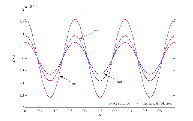
The computation is run with $p=0.01$. Fig. 1 describes the numerical solutions at different time compared to the exact solutions when $M=100$, $N=500$. As the graph shows, the exact and numerical solutions are in good agreement. Table 3 reports the global errors at $t=1$, $t=2$, and $t=3$ with various $M$, $N$. It is visible that Eqs. (3.17)-(4.18) well solve the test problem as expected.

Figure 1: The exact and numerical solutions at $t=1$, $3$, and $6$, when $M=100$, $N=500$.

Table 3: The global errors at different time with $p=0.01$ and various $M$, $N$ for Example 6.3

$M$, $N$	$||u-u_{N}||_{L^{2}}$			$||u-u_{N}||_{L^{\infty}}$
	$t=1$	$t=2$	$t=3$	$t=1$	$t=2$	$t=3$
32, 4000	5.4324e-5	3.8735e-5	3.1716e-5	8.8587e-5	6.3211e-5	5.1768e-5
64, 4000	1.3203e-5	9.6132e-6	7.9258e-6	2.1878e-5	1.5795e-5	1.2985e-5
128, 9000	3.0826e-6	2.3273e-6	1.9418e-6	5.2449e-6	3.8791e-6	3.2140e-6
256, 9000	5.3117e-7	4.7773e-7	4.2641e-7	9.5837e-7	8.4372e-7	7.3492e-7
1024, 250	5.9928e-6	2.1116e-6	1.1412e-6	9.4652e-6	3.3298e-6	1.7970e-6
1024, 500	3.6171e-6	1.2685e-6	6.8189e-7	5.6050e-6	1.9593e-6	1.0500e-6
2048, 1000	2.2589e-6	7.9847e-7	4.3255e-7	3.4336e-6	1.2092e-6	6.5273e-7
2048, 2000	1.4133e-6	4.9781e-7	2.6867e-7	2.1044e-6	7.3642e-7	3.9486e-7

Example 6.4. Let $\kappa=2$, $T=1$, $\varphi(x)=0$, $g_{1}(t)=0$, $g_{2}(t)=g_{1}(t)$, and the force function

$$f(x,t)=\frac{2t^{2-\alpha}x(1-x)\exp(x)}{\Gamma(3-\alpha)}+2t^{2}x(x+3)\exp(x);$$

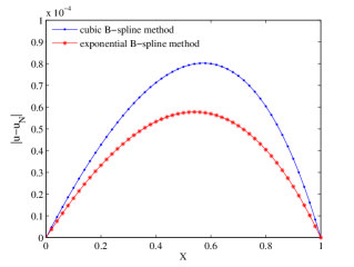
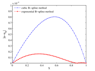
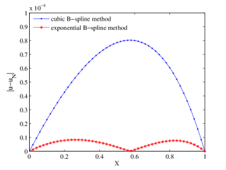
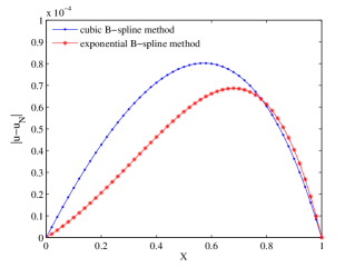
we consider Eqs. (1.1)-(1.3) on domain (0,1) solved by Eqs. (3.17)-(4.18) and the cubic B-spline collocation method (CBSCM) [32]. The exact solution of the model is $u(x,t)=t^{2}x(1-x)\exp(x)$. In Fig. 2, we display their absolute error distributions at $t=T$ when $\alpha=0.6$, $M=50$, $N=2500$ by taking $p=1.45$, $2.35$, $2.53$, and $3.35$, respectively. 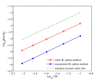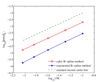In line with the graphs, we then choose $p=2.53$ and show a comparison of their absolute errors at some nodal points detailedly in Table 4, where the accuracy of our method is found to be overall better than CBSCM. In Fig. 3, we plot the global errors versus the variation of mesh size $1/M$ in log-log scale, with $\alpha=0.6$, $p=2.53$, and $N=11000$, which demonstrates the convergent orders of these methods are all basically of order $2$.

Figure 2: The absolute error distributions for $p=1.45$, $2.35$, $2.53$, and $3.35$ when $M=50$, $N=2500$.

Table 4: The comparison of absolute errors between CBSCM and our method when $p=2.53$.

x	$M=25$, $N=625$		$M=50$, $N=2500$
	CBSCM	our method	CBSCM	our method
0.1	7.4297e-5	1.7521e-5	2.2881e-5	5.2238e-6
0.2	1.7128e-4	3.1447e-5	4.2725e-5	7.8796e-6
0.3	2.2488e-4	3.3028e-5	5.9053e-5	8.1580e-6
0.4	2.8563e-4	2.5425e-5	7.1249e-5	6.3822e-6
0.5	3.1076e-4	1.5134e-5	7.8544e-5	3.0497e-6
0.6	3.2060e-4	4.5617e-6	7.9982e-5	1.1163e-6
0.7	3.0518e-4	1.7614e-5	7.4401e-5	5.1068e-6
0.8	2.4201e-4	3.0270e-5	6.0392e-5	7.5532e-6
0.9	1.6825e-4	2.8820e-5	3.6264e-5	6.6400e-6

Example 6.5. In the last test, we consider the fractional heat transfer model on $(0,1)$ with $\kappa=1$, $T=1$, $\varphi(x)=0$, $g_{1}(t)=0$, and $g_{2}(t)=H(t-0.2)-H(t-0.6)$, where $H(\cdot)$ denotes Heaviside Step Function. As in [25], the heat flux at the boundary point $x=0$ approximated by forward difference is of particular interest and the computed results are compared with the ones obtained by implicit finite difference method in the literature. 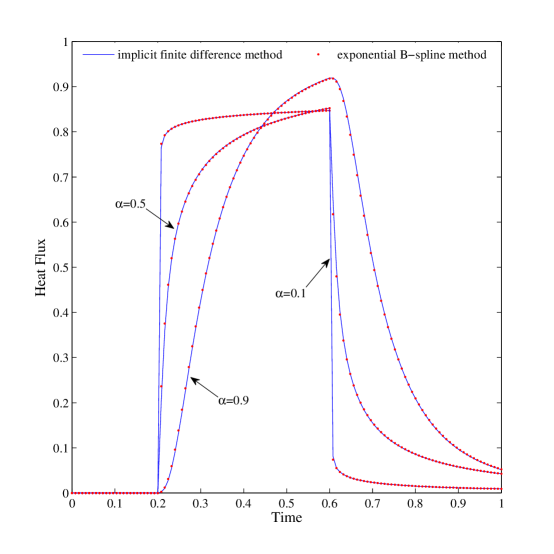Taking $p=1$, $M=500$, $N=125$, Fig. 4 exhibits the heat flux at $x=0$ changing over the time for $\alpha=0.1$, $0.5$, and $0.9$. It is clear that the results of these methods in presence are highly consistent, which reveals that our method precisely captures the heat flux.

7 Conclusion

In this research, an efficient exponential B-spline based collocation method is proposed to tackle the diffusion equation with a time-fractional derivative in Caputo sense discretized by a GMMP scheme. It leads to a linear system of algebraic equations with tri-diagonal coefficient matrix and thereby can be solved speedily by Thomas algorithm. The solvability is strictly evaluated and the stable analysis is proceeded by adopting a fractional von Neumann procedure. Its codes are tested on several given models and the numerical results validate that this method is capable of dealing with these equations very well. The comparison with the other methods manifests its practicability and advantages. Moreover, the derived method is easy and economical to carry out, so it can be served as an alternative choice to model the other fractional problems.

Figure 3: The convergent orders of the methods with $\alpha=0.6$, $p=2.53$, and $N=11000$.

Figure 4: The heat flux at $x=0$ for various $\alpha$ with $M=500$, $N=125$.

Acknowledgement: This research was supported by National Natural Science Foundations of China (No.11471262 and 11501450).

References

- Adams and Gelhar [1992] E.E. Adams, L.W. Gelhar, Field study of dispersion in a heterogeneous aquifer: 2. Spatial moments analysis, Water Res. Research 28 (1992) 3293–3307.
- Barkai [2002] E. Barkai, CTRW pathways to the fractional diffusion equation, Chem. Phys. 284 (2002) 13–27.
- Brunner et al. [2010] H. Brunner, L. Ling, M. Yamamoto, Numerical simulations of 2D fractional subdiffusion problems, J. Comput. Phys. 229 (2010) 6613–6622.
- Cui [2009] M.R. Cui, Compact finite difference method for the fractional diffusion equation, J. Comput. Phys. 228 (2009) 7792–7804.
- Deng [2007] W.H. Deng, Numerical algorithm for the time fractional Fokker-Planck equation, J. Comput. Phys. 227 (2007) 1510–1522.
- Deng et al. [2015] W.H. Deng, M.H. Chen, E. Barkai, Numerical algorithms for the forward and backward fractional Feynman-Kac equations, J. Sci. Comput. 62 (2015) 718–746.
- Gorenflo and Mainardi [1998] R. Gorenflo, F. Mainardi, Random walk models for space-fractional diffusion processes, Fract. Calc. Appl. Anal. 1 (1998) 167–191.
- Gorenflo et al. [2002] R. Gorenflo, F. Mainardi, D. Moretti, P. Paradisi, Time fractional diffusion: A discrete random walk approach, Nonlinear Dynam. 29 (2002) 129–143.
- Huang et al. [2015] C.B. Huang, X.J. Yu, C. Wang, Z.Z. Li, N. An, A numerical method based on fully discrete direct discontinuous Galerkin method for the time fractional diffusion equation, Appl. Math. Comput. 264 (2015) 483–492.
- Jiang and Ma [2011] Y.J. Jiang, J.T. Ma, High-order finite element methods for time-fractional partial differential equations, J. Comput. Appl. Math. 235 (2011) 3285–3290.
- Jin et al. [2015] B.T. Jin, R. Lazarov, J. Pasciak, Z. Zhou, Error analysis of semidiscrete finite element methods for inhomogeneous time-fractional diffusion, IMA J. Numer. Anal. 35 (2015) 561–582.
- Kilbas et al. [2006] A.A. Kilbas, H.M. Srivastava, J.J. Trujillo, Theory and Applications of Fractional Differential Equations, Amsterdam, 2006.
- Li and Wang [2009] C.P. Li, Y.H. Wang, Numerical algorithm based on adomian decomposition for fractional differential equations, Comput. Math. Appl. 57 (2009) 1672–1681.
- Li and Xu [2009] X.J. Li, C.J. Xu, A space-time spectral method for the time fractional diffusion equation, SIAM J. Numer. Anal. 47 (2009) 2108–2131.
- Lin and Xu [2007] Y.M. Lin, C.J. Xu, Finite difference/spectral approximations for the time-fractional diffusion equation, J. Comput. Phys. 225 (2007) 1533–1552.
- Liu et al. [2011] Q. Liu, Y.T. Gu, P.H. Zhuang, F.W. Liu, Y.F. Nie, An implicit RBF meshless approach for time fractional diffusion equations, Comput. Mech. 48 (2011) 1–12.
- Luo et al. [2016] W.H. Luo, T.Z. Huang, G.C. Wu, X.M. Gu, Quadratic spline collocation method for the time fractional subdiffusion equation, Appl. Math. Comput. 276 (2016) 252–265.
- Mainardi [1996] F. Mainardi, The fundamental solutions for the fractional diffusion-wave equation, Appl. Math. Lett. 9 (1996) 23–28.
- McCartin [1981] B.J. McCartin, Theory, Computation, and Application of Exponential Splines, Courant Mathematics and Computing Laboratory Research and Development Report, DOE/ER/03077-171, 1981.
- McCartin [1991] B.J. McCartin, Theory of exponential splines, J. Approx. Theory 66 (1991) 1–23.
- Meerschaert and Tadjeran [2004] M.M. Meerschaert, C. Tadjeran, Finite difference approximations for fractional advection-dispersion flow equations, J. Comput. Appl. Math. 172 (2004) 65–77.
- Metzler and Klafter [2000] R. Metzler, J. Klafter, The random walk’s guide to anomalous diffusion: A fractional dynamics approach, Phys. Rep. 339 (2000) 1–77.
- Momani and Odibat [2007] S. Momani, Z. Odibat, Numerical comparison of methods for solving linear differential equations of fractional order, Chaos. Soliton & Frac. 31 (2007) 1248–1255.
- Murillo and Yuste [2009] J.Q. Murillo, S.B. Yuste, On three explicit difference schemes for fractional diffusion and diffusion-wave equations, Phys. Scripta T136 (2009) 014025.
- Murio [2008] D.A. Murio, Implicit finite difference approximation for time fractional diffusion equations, Comput. Math. Appl. 56 (2008) 1138–1145.
- Nigmatulin [1986] R. Nigmatulin, The realization of the generalized transfer equation in a medium with fractal geometry, Phys. Stat. Sol. B 133 (1986) 425–430.
- Pirkhedri and Javadi [2015] A. Pirkhedri, H.H.S. Javadi, Solving the time-fractional diffusion equation via Sinc-Haar collocation method, Appl. Math. Comput. 257 (2015) 317–326.
- Podlubny [1999] I. Podlubny, Fractional Differential Equations, Academic Press, 1999.
- Povstenko [2010] Y. Povstenko, Signaling problem for time-fractional diffusion-wave equation in a half-space in the case of angular symmetry, Nonlinear Dynam. 59 (2010) 593–605.
- Ren et al. [2013] J.C. Ren, Z.Z. Sun, X. Zhao, Compact difference scheme for the fractional sub-diffusion equation with Neumann boundary conditions, J. Comput. Phys. 232 (2013) 456–467.
- Richardson [1926] L.F. Richardson, Atmospheric diffusion shown on a Distance-Nighbour graph, Proc. Roy. Soc. 110 (1926) 709–737.
- Sayevand et al. [2016] K. Sayevand, A. Yazdani, F. Arjang, Cubic B-spline collocation method and its application for anomalous fractional diffusion equations in transport dynamic systems, J. Vib. Control 22 (2016) 2173–2186.
- Yuste [2006] S.B. Yuste, Weighted average finite difference methods for fractional diffusion equations, J. Comput. Phys. 216 (2006) 264–274.
- Yuste and Acedo [2005] S.B. Yuste, L. Acedo, An explicit finite difference method and a new von Neumann-type stability analysis for fractional diffusion equations, SIAM J. Numer. Anal. 42 (2005) 1862–1874.
- Yuste and Murillo [2012] S.B. Yuste, J.Q. Murillo, A finite difference method with non-uniform timesteps for fractional diffusion equations, Comput. Phys. Commu. 183 (2012) 2594–2600.
- Zhuang et al. [2008] P. Zhuang, F. Liu, V. Anh, I. Turner, New solution and analytical techniques of the implicit numerical method for the sub-diffusion equation, SIAM J. Numer. Anal. 46 (2008) 1079–1095.
- Zhuang and Liu [2006] P.H. Zhuang, F.W. Liu, Implicit difference approximation for the time fractional diffusion equation, J. Comput. Appl. Math. 22 (2006) 87–99.