Forcer: a FORM program for 4-loop massless propagators

Abstract:

We present a new Form program for analytically evaluating four-loop massless propagator-type Feynman integrals in an efficient way. Our program Forcer implements parametric reductions of the aforementioned class of Feynman integrals into a set of master integrals and can be considered as a four-loop extension of the three-loop Mincer program. Since the program structure at the four-loop level is highly complicated and the equations easily become lengthy, most of the code was generated in an automatic way or with computer-assisted derivations. We have checked correctness of the program by recomputing already-known quantities in the literature.

1 Introduction

Evaluating multi-loop massless self-energy diagrams and related quantities is one of the typical problems in computing higher-order corrections to physical observables (see ref. [1] for a recent review). The Mincer program, firstly implemented [2] in Schoonschip [3] and later reprogrammed [4] in Form [5], was made for calculations of such integrals up to the three-loop level and has been used in many phenomenological applications.

The algorithm in the Mincer program is based on the following facts:

• A large part of integrals can be reduced into simpler ones via integration-by-parts identities (IBPs) [6, 7] of dimensionally regularized [8, 9] Feynman integrals. In particular, the so-called triangle rule, for which an explicit summation formula was given in ref. [10], can be applied to many of the cases in the class.

• One-loop massless integrals are easily performed and expressed in terms of G-functions [11, 7]. This also gives reductions of multi-loop integrals into those with one loop less but with non-integer powers of propagators.

After the whole reduction procedure, all integrals are expressed in terms of the gamma functions and two master integrals. Laurent series expansions of the latters with respect to the regulator $\epsilon$ were obtained by another method [11], where $D=4-2\epsilon$ is the number of space-time dimensions.

To perform massless propagator-type Feynman integrals at the four-loop level, there exist generic and systematic ways of the IBP reductions; these include: Laporta’s algorithm [12] (see [13, 14, 15, 16, 17, 18] for public implementations), Baikov’s method [19, 20] and heuristic search of the reduction rules [21, 22]. After the reduction to a set of master integrals, one can substitute the Laurent series expansions of the master integrals given in refs. [23, 24]. Those IBP solvers work for the four-loop calculations; however, the IBP reduction usually takes much time and can easily become the bottleneck of the computation. More efficient reduction programs are demanded especially when one considers extremely time-consuming calculations, for example, higher moments of the four-loop splitting functions and the Wilson coefficients in deep-inelastic scattering [25].

This work aims to develop a new Form program Forcer [26, 27], which is specialized for the four-loop massless propagator-type Feynman integrals and must be more efficient than using general IBP solvers. This is achieved by extending the algorithm of the three-loop Mincer program into the four-loop level. As the program can be highly complicated and error-prone at the four-loop level, the program should be generated in as automatic a way as possible, rather than coded by hand.

We specifically emphasize the following points that require automatization:

• Classification of topologies and constructing the reduction flow. All topologies appear at the four-loop level are enumerated and their graph structures are examined. The information is used for constructing the reduction flow from complicated topologies to simpler ones.

• Derivation of special rules. When substructures in a topology do not immediately give a reduction into simpler ones, one has to solve IBPs to obtain reduction rules for the topology, which removes at least one of the propagators or leads to a reduction into master integrals in the topology. They are obtained as symbolic rules, i.e., we allow the rules to contain indices (powers of the propagators and irreducible numerators) of the integrals as parameters.

The former can be fully automated by representing topologies as graphs in graph theory and utilizing several graph algorithms. In contrast, the latter is not trivial particularly when one considers the automatization. Much effort has been made for systematic search of symbolic rules using the Gröbner basis [28, 29] and the so-called s-basis [30, 31] as well as heuristics methods [21, 22]. Our approach for the special rules is more or less similar to ones in refs. [21, 22]. However, we constructed the reduction schemes for the special topologies with human intervention on top of computer-assisted derivations, often by trial and error for obtaining more efficient schemes. This was possible because in the Mincer/Forcer approach many topologies are reducible by rules derived from their substructures and we need special rules only for a limited number of topologies.

2 Constructing the reduction flow for all topologies

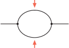
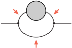
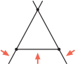
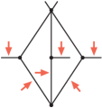
(a)	(b)	(c)	(d)

Figure 1: Substructures of topologies leading to reduction into simpler ones: (a) one-loop insertion, (b) one-loop carpet, (c) triangle and (d) diamond.

In order to manage many topologies appearing at the four-loop level, we need to automatize classification of topologies and constructing the reduction flow. We represent each topology as an undirected graph in graph theory, which makes it easy to detect the following types of substructures in a topology, depicted in figure 1, by pattern matchings of connections among vertices and edges:

1. One-loop insertion: the lines indicated by the arrows are integrated out.

2. One-loop carpet: the lines indicated by the arrows are integrated out.

3. Triangle: the triangle rule removes one of the three lines indicated by the arrows.

4. Diamond: the diamond rule [32] removes one of the six lines indicated by the arrows.

When none of the above is available, one has to solve the IBPs so as to obtain special rules.

Starting from the top-level topologies that consist of 3-point vertices, we consider removing a line from each topology in all possible ways. Massless tadpole topologies are immediately discarded. When a one-loop insertion/carpet is available in a topology, the loop integration can remove more than one line at a time, which should also be taken into consideration. For example, removing a line from the two lines in the one-loop topology gives a massless tadpole to be discarded, while removing both the two lines gives the Born graph. Some of generated topologies are often identical under graph isomorphism, which is efficiently detected by graph algorithms.

Irreducible numerators of a topology have to be chosen such that they do not interfere with the reduction determined by the topology substructure. Conversely, two topologies may have in general totally different sets of irreducible numerators, even if one is a derived topology obtained from the other by removing some of the lines and they have many common propagators. This means that a transition from a topology to another requires rewriting of irreducible numerators, which can be a bottleneck of computing complicated integrals with high powers of numerators.

Repeating this procedure until all topologies are reduced into the Born graph gives a reduction flow of all possible topologies. For the implementation, we used Python with a graph library igraph [33]. From 11 top-level topologies at the four-loop level, we obtained 437 non-trivial topologies in total. The numbers of topologies containing one-loop insertions, one-loop carpets, triangles and diamonds are 335, 24, 53 and 4, respectively. The remaining 21 topologies require construction of special rules.

3 Derivation of special rules

We start from the set of IBPs constructed in the usual way:

$$S_{0}=\{I_{1},\cdots,I_{R_{0}}\},$$ (1)

where each IBP is given as $I_{i}=0$ and the number of the relations is $R_{0}=L(L+E)$ for an $L$-loop topology with $E$-independent external momenta. We also define a set $S_{1}$ of IBPs obtained from $S_{0}$ with an index shifted by one in all possible ways. The set $S_{1}$ has $R_{1}=NR_{0}$ elements for a topology with $N$-indices. The set $S_{2}$ can be defined from $S_{0}$ by shifting an index by two or two indices by one. The sets $S_{3},S_{4},\dots$ may be defined in a similar way, but the number of the elements grows rather rapidly.

Then we consider searching useful reduction rules given by a linear combination of IBPs in the combined set of $S_{0}\cup S_{1}$:

$$\sum_{i}c_{i}I_{i}=0,\qquad I_{i}\in S_{0}\cup S_{1},$$ (2)

by trying to eliminate complicated integrals in the system. This may sound like the Laporta’s algorithm: defining sets of IBPs $S_{0},S_{1},\dots$ corresponds to generation of equations by choosing so-called seeds in the Laporta’s algorithm. Note that, however, we keep indices of integrals as parameters, unless we have already applied recursions to bring some of the indices down to fixed values (usually one or zero). The coefficients $c_{i}$ in eq. (2) may contain the indices as parameters. Although one could expect that including sets with higher shifts $S_{2},S_{3},S_{4},\dots$ makes the system overdetermined at some point, it never works because the coefficients can become immoderately complicated in an intermediate step of solving the system. Nevertheless, we observed that, with careful selection of linear combinations and of the order of reducing indices, in many cases the combined set $S_{0}\cup S_{1}$ is enough for obtaining reasonable rules and the complexity of coefficients in the rules can be under control.

A combination of reduction rules gives a reduction scheme of a topology into master integrals or simpler topologies. One needs criteria to select rules as components of a scheme, for example,

• Which index is reduced to a fixed value: bringing an index that entangles other indices in a complicated way down to a fix value often makes the reduction easy afterwards.

• Reducing complexity of integrals: it is ideal that recursion rules reduce the complexity of every integral at each step, which automatically guarantees the termination of the recursions.

• The number of terms generated by rules: a large number of generated terms in recursions are very stressful for computer algebra systems.

• Complexity of coefficients: as one uses exact rational arithmetic, complicated denominators of coefficients in generated terms considerably slow down the calculation. Moreover, spurious poles, which appear in denominators at intermediate steps but cancel out in the final result, can be problematic when one wants to expand and truncate the coefficients instead of using exact rational arithmetic during the calculation.

In practice, it is often difficult to find rules that satisfy all of the above criteria and one has to be reconciled to unsatisfactory rules at some extent. It is also true that predicting efficiency of a rule from its expression is non-trivial. Efficiency of reduction rules should be judged by how much it affects the total performance in adequate benchmark tests for the whole reduction scheme.

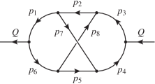
Figure 2: The three-loop non-planar topology.

3.1 Example: special rules for the three-loop non-planar topology

As an example, let us consider the three-loop non-planar topology (figure 2):

$$\operatorname{{\bf NO}}(n_{1},\dots,n_{9})=\int d^{D}p_{1}d^{D}p_{2}d^{D}p_{3}\frac{(Q\cdot p_{2})^{-n_{9}}}{(p_{1}^{2})^{n_{1}}\dots(p_{8}^{2})^{n_{8}}}.$$ (3)

The indices for the propagators take positive integer values: $n_{1}\geq 1,\dots,n_{8}\geq 1$, while the index $n_{9}$ for the irreducible numerator is negative: $n_{9}\leq 0$. When at least one of the indices for the propagators turns into a non-positive integer, the integral becomes one with a simpler topology. For simplicity, we set $Q^{2}=1$. As the set $S_{0}$, we have 12 IBPs, which are schematically given by

$$\begin{aligned} I_{1}&=\operatorname{{\bf IBP}}\left(\frac{\partial}{\partial p_{1}}\cdot p_{1},\operatorname{{\bf NO}}\right),&I_{2}&=\operatorname{{\bf IBP}}\left(\frac{\partial}{\partial p_{1}}\cdot p_{2},\operatorname{{\bf NO}}\right),&I_{3}&=\operatorname{{\bf IBP}}\left(\frac{\partial}{\partial p_{1}}\cdot p_{3},\operatorname{{\bf NO}}\right),\\ I_{4}&=\operatorname{{\bf IBP}}\left(\frac{\partial}{\partial p_{1}}\cdot Q,\operatorname{{\bf NO}}\right),&I_{5}&=\operatorname{{\bf IBP}}\left(\frac{\partial}{\partial p_{2}}\cdot p_{1},\operatorname{{\bf NO}}\right),&I_{6}&=\operatorname{{\bf IBP}}\left(\frac{\partial}{\partial p_{2}}\cdot p_{2},\operatorname{{\bf NO}}\right),\\ I_{7}&=\operatorname{{\bf IBP}}\left(\frac{\partial}{\partial p_{2}}\cdot p_{3},\operatorname{{\bf NO}}\right),&I_{8}&=\operatorname{{\bf IBP}}\left(\frac{\partial}{\partial p_{2}}\cdot Q,\operatorname{{\bf NO}}\right),&I_{9}&=\operatorname{{\bf IBP}}\left(\frac{\partial}{\partial p_{3}}\cdot p_{1},\operatorname{{\bf NO}}\right),\\ I_{10}&=\operatorname{{\bf IBP}}\left(\frac{\partial}{\partial p_{3}}\cdot p_{2},\operatorname{{\bf NO}}\right),&I_{11}&=\operatorname{{\bf IBP}}\left(\frac{\partial}{\partial p_{3}}\cdot p_{3},\operatorname{{\bf NO}}\right),&I_{12}&=\operatorname{{\bf IBP}}\left(\frac{\partial}{\partial p_{3}}\cdot Q,\operatorname{{\bf NO}}\right).\end{aligned}$$ (4)

We also build the set $S_{1}$ of 108 IBPs from $S_{0}$ by shifting $n_{i}\to n_{i}-1$ for all possible ways.

We solve the system consisting of $S_{0}\cup S_{1}$ by eliminating complicated integrals. First, we take a linear combination of IBPs as

$$\begin{split}&2I_{1}+4I_{6}+2I_{11}-I_{2}(n_{9}\to n_{9}+1)-2I_{6}(n_{9}\to n_{9}+1)-I_{10}(n_{9}\to n_{9}+1)\\ &+I_{2}(n_{1}\to n_{1}-1,n_{9}\to n_{9}+1)-I_{4}(n_{1}\to n_{1}-1,n_{9}\to n_{9}+1)\\ &-I_{4}(n_{2}\to n_{2}-1,n_{9}\to n_{9}+1)-2I_{8}(n_{2}\to n_{2}-1,n_{9}\to n_{9}+1)\\ &-I_{12}(n_{2}\to n_{2}-1,n_{9}\to n_{9}+1)+I_{10}(n_{3}\to n_{3}-1,n_{9}\to n_{9}+1)\\ &-I_{12}(n_{3}\to n_{3}-1,n_{9}\to n_{9}+1)-I_{10}(n_{4}\to n_{4}-1,n_{9}\to n_{9}+1)\\ &-I_{2}(n_{6}\to n_{6}-1,n_{9}\to n_{9}+1)+I_{4}(n_{7}\to n_{7}-1,n_{9}\to n_{9}+1)\\ &+I_{12}(n_{8}\to n_{8}-1,n_{9}\to n_{9}+1)=0,\end{split}$$ (5)

where $I_{i}(n_{j}\to n_{j}\pm 1,\dots)$ represents $I_{i}$ with the indices shifted. We have also globally shifted $n_{9}\to n_{9}+1$ in $S_{0}\cup S_{1}$. The linear combination in eq. (5) gives a rule

$$\begin{split}&\operatorname{{\bf NO}}(n_{1},n_{2},n_{3},n_{4},n_{5},n_{6},n_{7},n_{8},n_{9})=\frac{1}{2(n_{1}+n_{2}+n_{3}+n_{4}+n_{5}+n_{6}+n_{7}+n_{8}+n_{9}-7+4\epsilon)}\Bigl{[}\\ &+n_{1}\operatorname{{\bf NO}}({\color[rgb]{1,0,0}n_{1}+1},{\color[rgb]{0,0,1}n_{2}-1},n_{3},n_{4},n_{5},n_{6},n_{7},n_{8},{\color[rgb]{0,0,1}n_{9}+1})\\ &-n_{1}\operatorname{{\bf NO}}({\color[rgb]{1,0,0}n_{1}+1},n_{2},n_{3},n_{4},n_{5},n_{6},{\color[rgb]{0,0,1}n_{7}-1},n_{8},{\color[rgb]{0,0,1}n_{9}+1})\\ &+n_{3}\operatorname{{\bf NO}}(n_{1},{\color[rgb]{0,0,1}n_{2}-1},{\color[rgb]{1,0,0}n_{3}+1},n_{4},n_{5},n_{6},n_{7},n_{8},{\color[rgb]{0,0,1}n_{9}+1})\\ &-n_{3}\operatorname{{\bf NO}}(n_{1},n_{2},{\color[rgb]{1,0,0}n_{3}+1},n_{4},n_{5},n_{6},n_{7},{\color[rgb]{0,0,1}n_{8}-1},{\color[rgb]{0,0,1}n_{9}+1})\\ &+(n_{1}+2n_{2}+n_{3}+n_{9}-3+2\epsilon)\operatorname{{\bf NO}}(n_{1},n_{2},n_{3},n_{4},n_{5},n_{6},n_{7},n_{8},{\color[rgb]{0,0,1}n_{9}+1})\\ &+(n_{9}+1)\operatorname{{\bf NO}}(n_{1},{\color[rgb]{0,0,1}n_{2}-1},n_{3},n_{4},n_{5},n_{6},n_{7},n_{8},{\color[rgb]{0,0,1}n_{9}+2})\Bigr{]},\end{split}$$ (6)

which increases $n_{9}$ at least by one and can be repeatedly applied until $n_{9}$ becomes $0$. It also decreases the total complexity of integrals $\sum_{i=1}^{8}n_{i}-n_{9}$. The sum $\sum_{i=1}^{9}n_{i}$ appearing in the denominator is monotonically increased by one, therefore the coefficients get a single pole at most in the recursion. The last term increases $n_{9}$ by two, but due to its coefficient $(n_{9}+1)$, which vanishes when $n_{9}=-1$, it is guaranteed that $n_{9}$ never turns into a positive value.

Next, we set $n_{9}=0$ in the system and take a linear combination

$$\Bigl{[}-I_{1}(n_{1}\to n_{1}-1)+I_{4}(n_{1}\to n_{1}-1)-I_{6}(n_{1}\to n_{1}-1)+I_{7}(n_{1}\to n_{1}-1)\Bigr{]}\Bigr{|}_{n_{9}=0}=0,$$ (7)

which leads to

$$\begin{split}&\operatorname{{\bf NO}}(n_{1},n_{2},n_{3},n_{4},n_{5},n_{6},n_{7},n_{8},0)=\frac{1}{n_{1}-1}\Bigl{[}\\ &-n_{7}\operatorname{{\bf NO}}({\color[rgb]{0,0,1}n_{1}-1},n_{2},n_{3},{\color[rgb]{0,0,1}n_{4}-1},n_{5},n_{6},{\color[rgb]{1,0,0}n_{7}+1},n_{8},0)\\ &+n_{7}\operatorname{{\bf NO}}({\color[rgb]{0,0,1}n_{1}-1},n_{2},n_{3},n_{4},{\color[rgb]{0,0,1}n_{5}-1},n_{6},{\color[rgb]{1,0,0}n_{7}+1},n_{8},0)\\ &-n_{2}\operatorname{{\bf NO}}({\color[rgb]{0,0,1}n_{1}-1},{\color[rgb]{1,0,0}n_{2}+1},{\color[rgb]{0,0,1}n_{3}-1},n_{4},n_{5},n_{6},n_{7},n_{8},0)\\ &+n_{2}\operatorname{{\bf NO}}({\color[rgb]{0,0,1}n_{1}-1},{\color[rgb]{1,0,0}n_{2}+1},n_{3},n_{4},n_{5},n_{6},n_{7},{\color[rgb]{0,0,1}n_{8}-1},0)\\ &+(n_{1}+n_{2}+2n_{5}+2n_{6}+n_{7}+2n_{8}-9+4\epsilon)\operatorname{{\bf NO}}({\color[rgb]{0,0,1}n_{1}-1},n_{2},n_{3},n_{4},n_{5},n_{6},n_{7},n_{8},0)\\ &+(n_{1}-1)\operatorname{{\bf NO}}(n_{1},n_{2},n_{3},n_{4},n_{5},{\color[rgb]{0,0,1}n_{6}-1},n_{7},n_{8},0)\Bigr{]}.\end{split}$$ (8)

This rule decreases the total complexity as well as $(n_{1}+n_{6})$ and is applicable unless $n_{1}=1$. In fact, it is a variant of the diamond rule [32] and its existence is expected from the substructure of the topology. Similar rules exist for $n_{3}$, $n_{4}$ and $n_{6}$ due to the flipping symmetry of the topology. Eqs. (6) and (8) were used also in the original Mincer.

Lastly, we set $n_{1}=1$, $n_{3}=1$, $n_{4}=1$, $n_{6}=1$ and $n_{9}=0$. Then a solution of the system is obtained by the following linear combination:

$$\begin{split}&\Bigl{[}(n_{2}-1)I_{2}+(n_{2}-1)I_{6}+(n_{2}-1)I_{9}-(n_{2}-1)I_{10}+(n_{2}-1)I_{11}-(n_{2}-1)I_{12}\\ &+2(n_{2}-1)I_{1}(n_{1}\to n_{1}-1)-(n_{2}-1)I_{2}(n_{1}\to n_{1}-1)-(n_{2}-1)I_{4}(n_{1}\to n_{1}-1)\\ &+(n_{2}-1)I_{6}(n_{1}\to n_{1}-1)-(n_{2}-1)I_{8}(n_{1}\to n_{1}-1)+(n_{2}-1)I_{11}(n_{1}\to n_{1}-1)\\ &-(n_{2}-1)I_{12}(n_{1}\to n_{1}-1)+2(n_{2}-1)I_{1}(n_{2}\to n_{2}-1)-(n_{2}-1)I_{4}(n_{2}\to n_{2}-1)\\ &-2(n_{2}+2n_{5}+2n_{7}+n_{8}-6+4\epsilon)I_{5}(n_{2}\to n_{2}-1)\\ &+2(2n_{2}+2n_{5}+2n_{7}+n_{8}-7+4\epsilon)I_{6}(n_{2}\to n_{2}-1)\\ &-2(2n_{2}+2n_{5}+2n_{7}+n_{8}-7+4\epsilon)I_{7}(n_{2}\to n_{2}-1)\\ &+(3n_{2}+4n_{5}+4n_{7}+2n_{8}-13+8\epsilon)I_{8}(n_{2}\to n_{2}-1)\\ &-(n_{2}-1)I_{9}(n_{3}\to n_{3}-1)+(n_{2}-1)I_{10}(n_{3}\to n_{3}-1)-2(n_{2}-1)I_{11}(n_{3}\to n_{3}-1)\\ &+2(n_{2}-1)I_{12}(n_{3}\to n_{3}-1)-(n_{2}-1)I_{9}(n_{4}\to n_{4}-1)+(n_{2}-1)I_{10}(n_{4}\to n_{4}-1)\\ &+(n_{2}-1)I_{12}(n_{4}\to n_{4}-1)+2(n_{2}-1)I_{11}(n_{5}\to n_{5}-1)-(n_{2}-1)I_{12}(n_{5}\to n_{5}-1)\\ &-2(n_{2}-1)I_{1}(n_{6}\to n_{6}-1)-(n_{2}-1)I_{2}(n_{6}\to n_{6}-1)-3(n_{2}-1)I_{6}(n_{6}\to n_{6}-1)\\ &-(n_{2}-1)I_{11}(n_{6}\to n_{6}-1)+(n_{2}-1)I_{12}(n_{6}\to n_{6}-1)-2(n_{2}-1)I_{1}(n_{7}\to n_{7}-1)\\ &+(n_{2}-1)I_{4}(n_{7}\to n_{7}-1)-2(n_{2}-1)I_{6}(n_{7}\to n_{7}-1)+(n_{2}-1)I_{8}(n_{7}\to n_{7}-1)\\ &-2(n_{2}-1)I_{11}(n_{7}\to n_{7}-1)+(n_{2}-1)I_{12}(n_{7}\to n_{7}-1)-2(n_{2}-1)I_{1}(n_{9}\to n_{9}-1)\\ &+2(n_{2}-1)I_{5}(n_{9}\to n_{9}-1)-4(n_{2}-1)I_{6}(n_{9}\to n_{9}-1)-2(n_{2}-1)I_{11}(n_{9}\to n_{9}-1)\\ &+2(n_{2}-1)I_{12}(n_{9}\to n_{9}-1)\Bigr{]}\Bigr{|}_{n_{1}=n_{3}=n_{4}=n_{6}=1,n_{9}=0}=0,\end{split}$$ (9)

which gives

$$\operatorname{{\bf NO}}(1,n_{2},1,1,n_{5},1,n_{7},n_{8},0)=\frac{1}{(n_{2}-1)(n_{2}+n_{5}+n_{8}-3+2\epsilon)}\Bigl{\{}$$

$$-n_{7}(2n_{2}+2n_{5}+2n_{7}+n_{8}-7+4\epsilon)\operatorname{{\bf NO}}(1,{\color[rgb]{0,0,1}n_{2}-1},1,1,{\color[rgb]{0,0,1}n_{5}-1},1,{\color[rgb]{1,0,0}n_{7}+1},n_{8},0)$$

$$-n_{8}(2n_{5}+2n_{7}+n_{8}-5+4\epsilon)\operatorname{{\bf NO}}(1,{\color[rgb]{0,0,1}n_{2}-1},1,1,{\color[rgb]{0,0,1}n_{5}-1},1,n_{7},{\color[rgb]{1,0,0}n_{8}+1},0)$$

$$-\bigl{[}(n_{2}^{2}+4n_{2}n_{5}+2n_{2}n_{7}+3n_{2}n_{8}+4n_{5}^{2}+6n_{5}n_{7}+4n_{5}n_{8}+2n_{7}^{2}+3n_{7}n_{8}+n_{8}^{2}-11n_{2}-22n_{5}$$

$$\qquad-15n_{7}-12n_{8}+30)+(6n_{2}+12n_{5}+8n_{7}+6n_{8}-32)\epsilon+8\epsilon^{2}\bigr{]}$$

$$\qquad\quad\times\operatorname{{\bf NO}}(1,{\color[rgb]{0,0,1}n_{2}-1},1,1,n_{5},1,n_{7},n_{8},0)$$

$$-(n_{2}-1)(n_{5}+n_{8}-2+2\epsilon)\operatorname{{\bf NO}}(1,n_{2},1,1,{\color[rgb]{0,0,1}n_{5}-1},1,n_{7},n_{8},0)$$

$$+(n_{2}-1)(n_{2}+n_{5}+n_{8}-3+2\epsilon)\operatorname{{\bf NO}}(1,n_{2},1,1,n_{5},1,{\color[rgb]{0,0,1}n_{7}-1},n_{8},0)$$

$$-(n_{2}-1)(2n_{2}+2n_{5}+2n_{7}+n_{8}-7+4\epsilon)\operatorname{{\bf NO}}(1,n_{2},1,1,n_{5},1,n_{7},{\color[rgb]{0,0,1}n_{8}-1},0)$$

$$+n_{7}(2n_{2}+2n_{5}+2n_{7}+n_{8}-7+4\epsilon)\operatorname{{\bf NO}}(1,{\color[rgb]{0,0,1}n_{2}-1},1,{\color[rgb]{0,0,1}0},n_{5},1,{\color[rgb]{1,0,0}n_{7}+1},n_{8},0)$$

$$+n_{8}(2n_{2}+2n_{5}+2n_{7}+n_{8}-7+4\epsilon)\operatorname{{\bf NO}}(1,{\color[rgb]{0,0,1}n_{2}-1},1,1,n_{5},{\color[rgb]{0,0,1}0},n_{7},{\color[rgb]{1,0,0}n_{8}+1},0)$$

$$-2n_{8}(n_{2}-1)\operatorname{{\bf NO}}(1,n_{2},{\color[rgb]{0,0,1}0},1,n_{5},{\color[rgb]{0,0,1}0},n_{7},{\color[rgb]{1,0,0}n_{8}+1},0)$$

$$+(n_{2}-1)(2n_{2}+3n_{5}+2n_{7}+2n_{8}-9+6\epsilon)\operatorname{{\bf NO}}(1,n_{2},{\color[rgb]{0,0,1}0},1,n_{5},1,n_{7},n_{8},0)$$

$$+(n_{2}-1)(3n_{2}+2n_{5}+2n_{7}+2n_{8}-9+6\epsilon)\operatorname{{\bf NO}}(1,n_{2},1,1,n_{5},{\color[rgb]{0,0,1}0},n_{7},n_{8},0)\Bigr{\}}.$$ (10)

It decreases the total complexity by one and is applicable until $n_{1}=1$. Note that, because this rule is used when $n_{2}\geq 2$, $n_{5}\geq 1$ and $n_{8}\geq 1$, we have $(n_{2}+n_{5}+n_{8}-3)\geq 1$ and hence the coefficients never get any poles. There exist similar rules for $n_{5}$, $n_{7}$ and $n_{8}$. Consequently, all integrals in the three-loop non-planar topology are reduced into one master integral $\operatorname{{\bf NO}}(1,1,1,1,1,1,1,1,0)$ and integrals in simpler topologies.

4 Conclusion

We have developed a Form program Forcer for efficient evaluation of massless propagator-type Feynman integrals up to the four-loop level. It implements parametric reductions as Mincer does for three-loop integrals. Due to the complexity of the problem, many parts of the code is generated in automatic ways.

To check correctness of the program, we recomputed several known results in the literature, including the four-loop QCD $\beta$-function [34, 35] and lower moments of the four-loop non-singlet splitting functions [36, 37, 38, 1] (see also ref. [25]). Such recomputations also provide practical benchmark tests. By using the background field method with some tricks [39], the four-loop QCD $\beta$-function was recomputed within 10 minutes with dropping all gauge parameters and less than 9 hours with fully including gauge parameters (of course the final result is independent of the gauge parameter), on a decent 24 core machine. More physics results by Forcer will be reported elsewhere [40].

- [1] P.A. Baikov, K.G. Chetyrkin and J.H. Kühn, Massless propagators, and multiloop QCD, Nucl. Part. Phys. Proc. 261-262 (2015) 3 [arXiv:1501.06739].
- [2] S.G. Gorishny, S.A. Larin, L.R. Surguladze and F.V. Tkachov, Mincer: Program for multiloop calculations in quantum field theory for the SCHOONSCHIP system, Comput. Phys. Commun. 55 (1989) 381.
- [3] H. Strubbe, Manual for SCHOONSCHIP: A CDC 6000 / 7000 program for symbolic evaluation of algebraic expressions, Comput. Phys. Commun. 8 (1974) 1.
- [4] S.A. Larin, F.V. Tkachov and J.A.M. Vermaseren, The FORM version of MINCER, NIKHEF-H/91-18.
- [5] J. Kuipers, T. Ueda, J.A.M. Vermaseren and J. Vollinga, FORM version 4.0, Comput. Phys. Commun. 184 (2013) 1453 [arXiv:1203.6543].
- [6] F.V. Tkachov, A theorem on analytical calculability of 4-loop renormalization group functions, Phys. Lett. B100 (1981) 65.
- [7] K.G. Chetyrkin and F.V. Tkachov, Integration by parts: The algorithm to calculate -functions in 4 loops, Nucl. Phys. B192 (1981) 159.
- [8] C.G. Bollini and J.J. Giambiagi, Dimensional renormalization: The number of dimensions as a regularizing parameter, Nuovo Cim. B12 (1972) 20.
- [9] G. ’t Hooft and M.J.G. Veltman, Regularization and renormalization of gauge fields, Nucl. Phys. B44 (1972) 189.
- [10] F.V. Tkachov, An algorithm for calculating multiloop integrals, Theor. Math. Phys. 56 (1983) 866.
- [11] K.G. Chetyrkin, A.L. Kataev and F.V. Tkachov, New approach to evaluation of multiloop Feynman integrals: The Gegenbauer polynomial -space technique, Nucl. Phys. B174 (1980) 345.
- [12] S. Laporta, High precision calculation of multiloop Feynman integrals by difference equations, Int. J. Mod. Phys. A15 (2000) 5087 [hep-ph/0102033].
- [13] C. Anastasiou and A. Lazopoulos, Automatic integral reduction for higher order perturbative calculations, JHEP 07 (2004) 046 [hep-ph/0404258].
- [14] A.V. Smirnov, Algorithm FIRE – Feynman Integral REduction, JHEP 10 (2008) 107 [arXiv:0807.3243].
- [15] A.V. Smirnov and V.A. Smirnov, FIRE4, LiteRed and accompanying tools to solve integration by parts relations, Comput. Phys. Commun. 184 (2013) 2820 [arXiv:1302.5885].
- [16] A.V. Smirnov, FIRE5: a C++ implementation of Feynman Integral REduction, Comput. Phys. Commun. 189 (2014) 182 [arXiv:1408.2372].
- [17] C. Studerus, Reduze - Feynman integral reduction in C++, Comput. Phys. Commun. 181 (2010) 1293 [arXiv:0912.2546].
- [18] A. von Manteuffel and C. Studerus, Reduze 2 - distributed Feynman integral reduction, arXiv:1201.4330.
- [19] P.A. Baikov, Explicit solutions of the three loop vacuum integral recurrence relations, Phys. Lett. B385 (1996) 404 [hep-ph/9603267].
- [20] P.A. Baikov, A practical criterion of irreducibility of multi-loop Feynman integrals, Phys. Lett. B634 (2006) 325 [hep-ph/0507053].
- [21] R.N. Lee, Presenting LiteRed: a tool for the Loop InTEgrals REDuction, arXiv:1212.2685.
- [22] R.N. Lee, LiteRed 1.4: a powerful tool for reduction of multiloop integrals, J. Phys. Conf. Ser. 523 (2014) 012059 [arXiv:1310.1145].
- [23] P.A. Baikov and K.G. Chetyrkin, Four loop massless propagators: An algebraic evaluation of all master integrals, Nucl. Phys. B837 (2010) 186 [arXiv:1004.1153].
- [24] R.N. Lee, A.V. Smirnov and V.A. Smirnov, Master integrals for four-loop massless propagators up to transcendentality weight twelve, Nucl. Phys. B856 (2012) 95 [arXiv:1108.0732].
- [25] B. Ruijl, T. Ueda, J.A.M. Vermaseren, J. Davies and A. Vogt, First Forcer results on deep-inelastic scattering and related quantities, these proceedings, arXiv:1605.08408.
- [26] T. Ueda, B. Ruijl and J.A.M. Vermaseren, Calculating four-loop massless propagators with Forcer, to appear in proceedings of the 17th International workshop on Advanced Computing and Analysis Techniques in physics research (ACAT 2016), Valparaiso, Chile, January 18-22, 2016, arXiv:1604.08767.
- [27] B. Ruijl, T. Ueda and J.A.M. Vermaseren, in preparation.
- [28] O.V. Tarasov, Reduction of Feynman graph amplitudes to a minimal set of basic integrals, Acta Phys. Polon. B29 (1998) 2655 [hep-ph/9812250].
- [29] V.P. Gerdt, Grobner bases in perturbative calculations, Nucl. Phys. Proc. Suppl. 135 (2004) 232 [hep-ph/0501053].
- [30] A.V. Smirnov and V.A. Smirnov, S-bases as a tool to solve reduction problems for Feynman integrals, Nucl. Phys. Proc. Suppl. 160 (2006) 80 [hep-ph/0606247].
- [31] A.V. Smirnov, An algorithm to construct Grobner bases for solving integration by parts relations, JHEP 04 (2006) 026 [hep-ph/0602078].
- [32] B. Ruijl, T. Ueda and J. Vermaseren, The diamond rule for multi-loop Feynman diagrams, Phys. Lett. B746 (2015) 347 [arXiv:1504.08258].
- [33] G. Csardi and T. Nepusz, The igraph software package for complex network research, InterJournal Complex Systems (2006) 1695, http://igraph.org.
- [34] T. van Ritbergen, J.A.M. Vermaseren and S.A. Larin, The four-loop -function in quantum chromodynamics, Phys. Lett. B400 (1997) 379 [hep-ph/9701390].
- [35] M. Czakon, The four-loop QCD -function and anomalous dimensions, Nucl. Phys. B710 (2005) 485 [hep-ph/0411261].
- [36] P.A. Baikov and K.G. Chetyrkin, New four loop results in QCD, Nucl. Phys. Proc. Suppl. 160 (2006) 76.
- [37] V.N. Velizhanin, Four loop anomalous dimension of the second moment of the non-singlet twist-2 operator in QCD, Nucl. Phys. B860 (2012) 288 [arXiv:1112.3954].
- [38] V.N. Velizhanin, Four loop anomalous dimension of the third and fourth moments of the non-singlet twist-2 operator in QCD, arXiv:1411.1331.
- [39] F. Herzog, B. Ruijl, T. Ueda, J.A.M. Vermaseren and A. Vogt, Form, diagrams and topologies, these proceedings.
- [40] B. Ruijl, T. Ueda, J.A.M. Vermaseren and A. Vogt, in preparation.
- [41] J.C. Collins and J.A.M. Vermaseren, Axodraw version 2, arXiv:1606.01177.