Minimal model for spontaneous quantum synchronization

Abstract

We show the emergence of spontaneous synchronization between a pair of detuned quantum oscillators within a harmonic network. Our model does not involve any nonlinearity, driving or external dissipation, thus providing the simplest scenario for the occurrence of local coherent dynamics in an extended harmonic system. A sufficient condition for synchronization is established building upon the Rayleigh’s normal modes approach to vibrational systems. Our results show that mechanisms favoring synchronization, even between oscillators that are not directly coupled to each other, are transient energy depletion and cross-talk. We also address the possible build-up of quantum correlations during synchronization and show that indeed entanglement may be generated in the detuned systems starting from uncorrelated states and without any direct coupling between the two oscillators.

I Introduction

Synchronization among dynamical systems is a widespread phenomenon which has been widely studied in the classical domain and, more recently, in the quantum regime SynchQ ; sync2012 ; syncSR ; fazio1 . Indeed, synchronization is a relevant phenomenon in several contexts, including physical, biological, chemical and social systems, and it has been also generalized to a large variety of dynamical regimes, from regular oscillations to chaotic evolutions stro93 ; osi07 ; Pikovsky ; Strogatz ; manb . These investigations have extended the definition of synchronization, showing that mutual or directional coupling between inhomogeneous components, are relevant for its occurrence, as well as non-linearity, dissipation, noise, forcing, or time delay. Overall, synchronization emerges as a paradigmatic phenomenon in complex systems Pikovsky .

The extension of the synchronization concept to the quantum case is not straightforward, since dynamical trajectories of the observables are not well defined and the very quantum properties of the canonical variables prevent the exact fulfillment of the classical conditions defining synchronization fazio1 ; synch_chapter . In turn, the appearance of quantum synchronization has been proved to be different from the appearance of coherence (as entanglement) and a question arises on how, whether and when the two phenomena may coexist.

In this framework, the question about the necessary ingredients to observe spontaneous synchronization in simpler dynamical models was less explored. While in a classical setting, synchronization is mostly studied for nonlinear systems, in a recent work on the synchronization of quantum fluctuations sync2012 , it was shown that it can actually arise even in linear models, solely due to dissipation, and it may persist asymptotically for larger systems syncLalo ; syncSR .

In this work we introduce and discuss a minimal model for the emergence of synchronization, in systems with no external forcing, nonlinear effects, and dissipation. More specifically, we consider an isolated linear network of coupled harmonic oscillators and address the emergence of coherent dynamics, i.e. synchronization, in the subsystem made of a pair of nodes. In fact, harmonic network, besides being fundamental ingredients for modeling open quantum systems weiss-breuer , are of interest for a broad spectrum of topics ranging from consensus problems arenas to trapped ions ions .

In general, harmonic networks models of extended environments, even in the weak coupling limit, lead to a rather complex dissipation mechanisms for the embedded subsystems ruggero ; johannes ; huelga ; burghardt , including several different spatial effects when the system is multipartite CBSB ; vega . Our physical model involves a large isolated network of oscillators and within this description, we analyze dissipation-induced synchronization. Besides, we provide a sufficient condition for the emergence of synchronization between detuned nodes in the framework of the physics of vibrations and in the limit of the Rayleigh approximation.

In a second part of our work we analyze the strong coupling regime, where the two nodes under investigation are strongly coupled to the rest of the network. This is still a linear model amenable to analytic solution. Clearly, if one excites only one normal mode, some network nodes will oscillate synchronously, but this in not the case under study here. We consider instead a generic initial condition exciting the two probes. Here, the mechanisms governing the transport of energy as well as the possible scenarios for the emergence of synchronization are far to be trivial, being typically limited to temporal transients and susceptible to variations in couplings, inhomogeneities and boundary effects. In particular, we present and discuss two different routes to synchronization mediated by the environment in a simple chain configuration. In addition, we analyze in some details the possible build-up of quantum correlations during synchronization, showing that entanglement may be generated in our detuned systems starting from uncorrelated states and without any direct coupling between the two oscillators.

Indeed, synchronization in itself is defined using classical temporal averages also for quantum systems. However, all the synchronization scenarios mentioned above are not specific of classical systems, being not limited to first order moments. In fact, quantum noise synchronization in presence of squeezing has been already reported sync2012 ; syncSR , upon considering local variances. We thus devote the final Section to address the possible emergence of quantum signatures, and analyze the dynamics of quantum correlations and the possible build-up of mutual information and entanglement when starting from uncorrelated product states. The possibility to generate quantum correlations through bosonic baths has been already considered in the literature. In particular, ion chains acting as reservoirs have been recently shown to mediate entanglement between identical ions defects, when placed in one edge morigiY and also at a distance morigiEPL while entanglement generation via a heat bath could not be established between remote objects in Ref. klesse . Here we take a further step extending previous analysis to non-uniform systems (being the system components detuned), allowing for strong system-environment coupling correa , and establishing the connections with a coherent (synchronous) dynamics sync2012 ; fazio1 ; fazio2 .

The paper is structured as follows. In Section II we introduce our model and establish notation. We also illustrate the quantitative measure of synchronization used throughout the paper and the Langevin equation governing the dynamics of the pair of oscillators. In Section III we discuss a general condition for synchronization and illustrate our results about synchronization via weak dissipation or across the chain. In Section IV we show the results obtained in the strong coupling regime and discuss synchronization by coupling to a common chain mode or by cross-talk. Finally, in Section V we show our results about the links between synchronization and the build-up of quantum correlations for the oscillators coupled to a common chain node or to the chain edges. Section VI closes the paper with some concluding remarks.

II Dynamical model

We consider a large network of $M$ coupled harmonic oscillators of unit mass described by the Hamiltonian ($\hbar=1$)

$$H_{E}=\sum_{j=1}^{M}\frac{1}{2}(P_{j}^{2}+\Omega_{0}^{2}X_{j}^{2})+\sum_{j,k=1}^{M}A_{jk}(X_{j}-X_{k})^{2}\,.$$

Besides, we address a system of two detuned oscillators, coupled to a pair of nodes of the network with strength $K$, and coupled between them with strength $\lambda$. The dynamics of the overall system is governed by the Hamiltonian $H=H_{S}+H_{E}+H_{I}$, with

$$H_{S} = \frac{1}{2}(p_{1}^{2}+p_{2}^{2})+\frac{1}{2}(\omega_{1}^{2}x_{1}^{2}+\omega_{2}^{2}x_{2}^{2})+\frac{\lambda}{2}(x_{1}-x_{2})^{2}$$ (1)

$$H_{I} = K(x_{1}\,X_{m}+x_{2}\,X_{n}),$$ (2)

where $n,m\in[1,M]$ are the positions within the network, where the two detuned oscillators are plugged. The canonical operators for the oscillators in the chain are denoted by capital letters $[X_{j},P_{k}]=i\delta_{jk}$, $[X_{j},X_{k}]=0$, $[P_{j},P_{k}]=0$, $j,k=1,M$ whereas $[x_{j},p_{k}]=i\delta_{jk}$, $[x_{j},x_{k}]=0$, $[p_{j},p_{k}]=0$, $j,k=1,2$ are the operators for the two detuned oscillators (at frequencies $\omega_{j}$, $j=1,2$). The (common) natural frequency of the oscillators in the network is denoted by $\Omega_{0}$ and the matrix $A_{jk}$ contains information about their couplings.

In the limit of $M\rightarrow\infty$ and decoupled oscillators, i.e. $\lambda=0$, this is a well-known framework for open quantum systems weiss-breuer and can be used to microscopically derive generalized Langevin equations for the reduced system dynamics hanggi . In this framework, one considers a set of independent degrees of freedom in the environment—the environmental normal modes $Q_{n}$—and assumes a certain spectral density, encoding the form of the coupling between system and environment as well as the spectral distribution of the latter. However, one can go beyond phenomenological assumptions and derive the spectral density associated to more complex configurations of coupled HOs, constituting different kind of finite networks rubin ; burghardt ; ruggero ; johannes . The case of a homogeneous chain, i.e. $A_{jk}=g\delta_{|j-k|,1}$, is particularly interesting because it allows (i) to reproduce an Ohmic dissipation rubin and (ii) to have a clear picture of the transport dynamics. On the other hand, increasing the environment complexity allows to engineer arbitrarily complex spectral densities, as in Refs.burghardt ; ruggero ; johannes , exhibiting non-Markovian effects huelga ; NMrev .

II.1 Synchronization

Mutual synchronization arises when, in spite of their detuning, the pair of oscillators starts to oscillate coherently, at a common frequency. A quantitative estimation of synchronization comes from a Pearson’s correlation among two time dependent functions $f,g$, namely

$$\mathcal{C}_{f,g}(t,\Delta t)=\overline{\delta f\delta g}/\sqrt{\overline{\delta f^{2}}~{}\overline{\delta g^{2}}}$$ (3)

where the bar stands for a time average

$$\overline{f}=\int_{t}^{t+\Delta t}dt^{\prime}f(t^{\prime})$$

within a time window $\Delta t$ and $\delta f=f-\overline{f}$. This is an indicator measuring the presence of dynamical synchronization between either classical trajectories Pikovsky or quantum systemssync2012 characterized by average positions, variances, and, possibly higher order moments. Other indicators of synchronization consider different forms of correlations between the nodes as in Refs. fazio1 ; fazio2 .

As recently reported sync2012 ; syncSR , a system of two (or more) HOs weakly dissipating into an infinitely large thermal bath ($M\rightarrow\infty$) displays synchronous dynamics when one normal mode is more protected against dissipation than the other(s) CBSB . In other words, synchronization emerges when all but one modes are largely damped and the dynamics is then governed by the eigenfrequency of the most robust mode syncLalo ; syncSR . The general condition derived for synchronization in the presence of a weakly coupled and infinite bath is indeed the presence of a gap between the damping rate of the two least damped modes of the system syncSR . For a finite environment and beyond weak coupling, the scenario is more complex but richer and our first step is to identify a similar mechanism for the emergence of synchronization, see Section III.

II.2 Dynamics

The dynamics of the subsystem of detuned oscillators, from now on referred to as the system, is governed by a pair of integro-differential equations. First and second order moments of the operators $(x_{j}$, $p_{j})$, $j=1,2$ are sufficient to fully characterize Gaussian states and their dynamics. We thus start by considering the average positions of the system oscillators $\langle x_{1,2}(t)\rangle$, whose dynamics is governed by generalized quantum Langevin equations weiss-breuer ; hanggi . These integro-differential equations depend on the structure and state of the overall network, and for the normal modes $q_{1,2}$ of the system they read as follows (see Appendix A)

$$\langle\ddot{q}_{1}(t)\rangle+\int_{0}^{t}dt^{\prime}[\gamma_{1}(t-t^{\prime})\langle\dot{q}_{1}(t^{\prime})\rangle+\eta(t-t^{\prime})\langle\dot{q}_{2}(t^{\prime})\rangle]$$

$$+\Lambda^{2}_{1}\langle q_{1}(t)\rangle-\gamma_{1}(0)\langle q_{1}(t)\rangle-\eta(0)\langle q_{2}(t)\rangle=0$$

Analogously, an equivalent equation is found for $\langle{q}_{2}\rangle$ by replacing $1\leftrightarrow 2$. Here the network features are encoded in the time-dependent coefficients $\gamma_{s}$ ($s=1,2$) and $\eta$, while $\Lambda_{1,2}$ are $H_{S}$ eigenfrequencies and we assume $\langle q_{1,2}(0)\rangle=0$ as initial conditions.

We emphasize that the system normal modes $q_{1,2}$ diagonalize $H_{S}$ but they remain dynamically coupled through damping, due to the interaction with the environment. In fact, the damping kernel contains different components; the first one is given by

$$\gamma_{s}(t-t^{\prime}) = \sum_{j=1}^{M}\frac{c_{s}^{2}(j)}{\Omega_{j}^{2}}\cos[\Omega_{j}(t-t^{\prime})]\Theta(t-t^{\prime}),$$ (4)

with $s=1,2$, and governs the local damping at each node as well as the possible feedback from the boundaries of the finite chain. The second terms reads as follows

$$\eta(t-t^{\prime}) = \sum_{j=1}^{M}\frac{c_{1}(j)c_{2}(j)}{\Omega_{j}^{2}}\cos[\Omega_{j}(t-t^{\prime})]\Theta(t-t^{\prime})$$ (5)

and introduces cross effects in the friction, through the transmission of signals among the system components along the chain. For this reason the $\eta$ coefficient is symmetric. The mathematical expressions for the $c_{s}(j)$ and $\Omega_{j}$ coefficients are given in Appendix A. The initial state for the network is the fundamental one ($T=0$), being the initial energy excitation localized in the system oscillators only.

III A sufficient condition for synchronization

The time non-local dissipation term in Eq. (II.2) may be approximated by a time local one, i.e. constant, damping, only in specific situations hanggi ; Kimble . This is usually the case when the system is weakly coupled to the rest of the network though, strictly speaking, each configuration of the network should be studied in details to understand whether and when a time local description is appropriate, at least during a transient time. If these conditions are fulfilled the dynamics of the system is described by a set of coupled differential equations of the form

$$\langle{\bf\ddot{x}}\rangle+G\langle{\bf\dot{x}}\rangle+A\langle{\bf x}\rangle=0\,,$$ (6)

where $\bf x={x_{1},x_{2}}$ and $A$ and $G$ are time-independent matrices. An interesting question, addressed earlier by Lord Rayleigh Ray in the context of the vibration of structures Ray ; vibrations is whether normal modes may be individuated in spite of the presence of dissipation. The undamped dynamics follows from a superposition of normal modes obtained diagonalizing the stiffness matrix $G$ and the coupling one $A$ in Eq. (6), but the specific form of damping mines this description because, in general, $A$ and $G$ cannot be simultaneously diagonalized.

As a matter of fact Ray ; Caugh , classical normal modes clmode are present if the matrices $A$ and $G$ commute. This leads to a simple description for the independently damped normal modes of the free dynamics (${\bf q}=(q_{1},q_{2})$). Small deviations from the condition $[G,A]=0$ justify the Rayleigh’s approximation of neglecting the non-diagonal components of $G$ in the basis of ${\bf q}$. This corresponds to the so-called reduction method Ray of disregarding out-of-diagonal terms of $G^{\prime}=M^{-1}GM$, where $M=(\{q_{1}\},\{q_{2}\})$ diagonalizes $A$ ($A^{\prime}=M^{-1}AM$), which is useful when dissipation is small. The approximation is equivalent to neglect the small cross damping among natural vibrations and, of course, the validity of this approach depends on the relative size when comparing with self-dampings. An example is shown in Ref.Galve and based on a secular approximation. The model described in Eq.(6), simplified under Rayleigh’s approximation, allows for a necessary and sufficient condition for synchronization: a pair of detuned oscillators embedded into a network will synchronize if there exists a gap between the normal mode damping rates $G^{\prime}_{11}$ and $G^{\prime}_{22}$. This condition is general for dissipation in infinite baths syncSR while for finite systems it is limited to the transient where the average dynamics of the pair of oscillators can be approximated by Eq. (6). Significant build-up of synchronization requires the least damped mode to be suppressed and this phenomenon should occur in a time scale of the order of the inverse of the larger damping

$$\tau_{S}^{-1}\sim\max(|G^{\prime}_{11}|,|G^{\prime}_{22}|).$$ (7)

In the following Section, we consider a finite chain configuration and provide and example of application of the above condition.

III.1 Synchronization via weak dissipation

Let us now consider a network made of a chain of $M$ oscillators homogeneous in frequency and couplings. The Hamiltonian is given by

$$H_{E}=\sum_{j=0}^{M}\frac{p_{j}^{2}}{2}+\frac{1}{2}\Omega_{0}^{2}X_{j}^{2}+\frac{g}{2}(X_{j}-X_{j+1})^{2}\,.$$

The network acts as an environment for a system made of two oscillators attached at one edge of the chain. The interaction Hamiltonian reads as follows

$$H_{I}=K(x_{1}+x_{2})X_{1}.$$ (8)

In this configuration only $x_{+}=x_{1}+x_{2}$ is directly coupled to the chain and $x_{\pm}$ diagonalize the damping term, while the system Hamiltonian $H_{S}$ is diagonal in $q_{1,2}$.

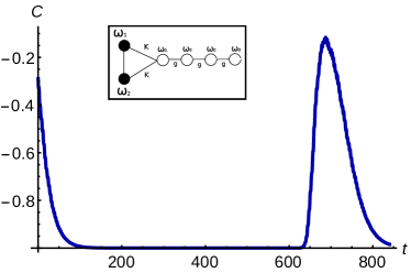
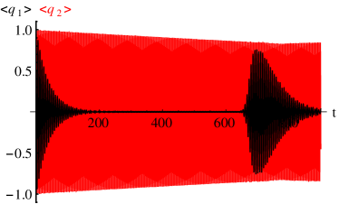
Figure 1: Synchronization measure $C(t)$ and dynamics for $\omega_{2}/\omega_{1}=1.1$, $\lambda=0.5\,\omega_{1}^{2}$, $x_{1}(0)=0.14\,\omega_{1}^{-1/2}$; $x_{2}(0)=1.4\,{\omega_{1}}^{-1/2}$, $M=300$, $\Omega_{0}=0.4\,\omega_{1}$, $g=1.2\,\omega_{1}^{2}$, $K=0.2\,\omega_{1}^{2}$. In the lower panel the black line denotes the function $\langle q_{1}(t)\rangle$ and the red one is for $\langle q_{2}(t)\rangle$. $\langle q_{1,2}\rangle$ are in units of $\omega_{1}^{-1/2}$ and time is in unit of $\omega_{1}^{-1}$.

In the limit of an infinitely large chain and vanishing local potential ($\Omega_{0}\simeq 0$) the environment acts as an Ohmic bath and the ratio between the damping rates is

$$G^{\prime}_{11}/G^{\prime}_{22}\simeq\frac{1+\sin 2\theta}{1-\sin 2\theta}$$ (9)

where the parameter $\theta$ depends upon the detuning and the coupling $\lambda$ (see Appendix A). The sufficient condition for transient synchronization is the presence of a gap between the normal modes damping, as it happens for small detuning, i.e. $|\omega_{1}-\omega_{2}|^{2}/\lambda<1$ in the case of Fig. 1 where $\sin 2\theta\simeq 1$. The synchronization measure $\mathcal{C}$ in this case shows that perfect anti-synchronization is present up to the revival time $\tau_{R}\sim 2M/\omega_{1}$. If the coupling of one of the oscillators to the chain switches from attractive to repulsive, $K\,x_{2}X_{1}\rightarrow-K\,x_{2}X_{1}$ in Eq.(8), then the quantity $x_{-}=x_{1}-x_{2}$ couples to the chain and synchronization instead of anti-synchronization arises.

As a matter of fact, during the initial transient time finite size effects can be neglected and the energy of the two system’s oscillators flows into the environmental chain en_flow , leading to an effective dissipation into a common bath sync2012 ; syncSR . Therefore, the neat build-up of anti-synchronization of Fig. 1 is consistent with the predicted phenomenon of Ref. sync2012 , where an infinite bath was considered. Boundary effects cause a departure from the Ohmic dissipation (constant damping in Eq.II.2) leading to revivals. Fig.1 shows that reflection from the boundary at $t=\tau_{R}$ actually deteriorates the coherent dynamics between the pair of HOs, and similar results are found when there are defects in the chain causing feedback effects at shorter times. This is accompanied by a regrowth in the oscillation amplitude of the damped mode $q_{1}$. The loss of anti-synchronization is indeed due to a common forcing toward synchronization due to the feedback signal reflected at the edge of the chain. At later times ($t>\tau_{R}$), after a competition transient, anti-synchronization is restored under the effect of dissipation, as shown in Fig.1, lasting until feedback effects arise again at $t\sim 2\tau_{R}$.

III.2 Synchronization across the chain

A natural question is what happens when moving the second oscillator through the chain with system-environment interaction

$$H_{I}=Kx_{1}X_{1}+Kx_{2}X_{m}~{}~{}~{}~{}~{}~{}~{}m\in[1,M].$$ (10)

The dependence of dissipation with the distance ($m$) in the weak coupling regime has been described elsewhere CBSB for infinite environment and a periodic transition between dissipation in common and separate baths has been predicted. The case under study differs due to finite size effects: reflections from the boundaries and cross-talk between the oscillators and feedback signals lead to a dynamics which strongly depends on the plugging distance $m$, and perfect synchronization may arise or not just by moving the system components from one site to the neighbor one. Still, this sensitivity to the plugging position is absent during a transient when $0\ll m\ll N$, i.e. second oscillator far from the first one and form the edge of the chain. More details are given in Appendix B.

IV Synchronization in strong coupling regime

The mechanism of synchronization by dissipation is enabled by the presence of coupling between the system oscillators (i.e. $\lambda\neq 0$) and it is consistent with results obtained for infinite environments sync2012 ; syncSR . An interesting question is the possibility to synchronize detuned oscillators in the absence of a direct coupling between them, i.e. $\lambda=0$, solely due to the mediating effect of the rest of the network. This was actually shown to be possible for spins in Ref.GLPlastina but it does not occur for weakly coupled harmonic oscillators. Indeed, for the oscillators pair attached to a common node, the dissipation mechanism described above does not produce synchronization in the weak coupling regime. Inspection of the master equation in sync2012 shows that, even for long chains (large $\tau_{R}$) the effective coupling induced by the bath (Lamb shift) is actually too small to lead to significant synchronization before the system thermalizes. On the other hand, a full system-bath model allows one to address less explored strong dissipation regimes enabling new dynamical scenarios for synchronization that are not present for weak coupling.

IV.1 Coupling to a common chain node

We now consider a configuration where the system is attached to one edge of the environment chain, as in Eq.(8), but now the two oscillators are uncoupled, $\lambda=0$. We allow for a frequency detuning $\omega_{1}\neq\omega_{2}$ implying that $x_{\pm}$ are not the eigenmodes of $H_{S}$. Up to the revival time $\tau_{R}$, the system oscillators will dissipate into the common environment and no synchronization is possible for weak coupling, i.e. $K\ll\omega_{i}^{2}$). Under-damped detuned oscillations characterize the dynamics at all times and the system components $x_{1},x_{2}$ remain incoherent.

This is not the case when $K\lesssim\omega_{i}^{2}$. We first notice that this rather large dissipation does not completely deplete the system energy. Indeed, after a fast transient oscillatory decay, the system achieves a steady regime of rather large oscillations with constant amplitude that last up the revival time. $\tau_{R}\simeq 600/\omega_{1}$ for the choice of parameters of Fig. 2. In this regime, oscillations are coherent at frequency smaller than the system frequencies ($0.4<\omega_{1,2}$, Fig. 2 bottom right) and perfect synchronization emerges. After the transmission of the initial pulse, originated at the edge of the chain, the stiff coupling ($K=0.8\,\omega_{1}^{2}$ in Fig.2) to the environment leads to a steady state in which the system vibrates at the lowest frequency of the chain, $\Omega_{0}=0.4\,\omega_{1}$. For decreasing coupling the system depletion of energy continues until complete damping, whereas for weaker coupling (e.g. $K=0.1\,\omega_{1}^{2}$) the system shows under-damped oscillation at the detuned (Lamb shifted) natural detuned frequencies, so no synchronization is established. This scenario of synchronization occurs for uncoupled probes stiffly attached to one node of a network until signal reflections (depending on the network topology) drive the system away from coherent oscillation, as shown here at the revival time.

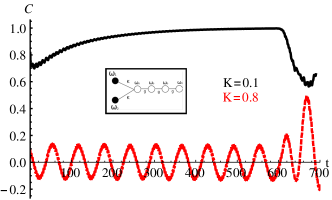
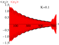
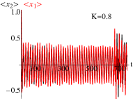
Figure 2: Upper plot: synchronization measure $C(t)$ as a function of time for two different values of the coupling $K=0.1$ (solid black) and $0.8$ (dotted red), in unit of $\omega_{1}^{2}$. The other parameters are fixed: $\omega_{2}/\omega_{1}=1.1$, $\lambda=0$, $M=300$, $\Omega_{0}=0.4\,\omega_{1}$, and $g=1.2\,\omega_{1}^{2}$. In the inset, we show a schematic representation of the considered configuration. Lower plot: dynamics of the two oscillators plugged into the first node of the chain, with $K=0.1$ (left panel) and $K=0.8$, in unit of $\omega_{1}^{2}$ (right panel). $\langle x_{1,2}\rangle$ are in units of $\omega_{1}^{-1/2}$ and time in units of $\omega_{1}^{-1}$.

IV.2 Synchronization by cross-talk

The phenomena described in Sect. III.1 and IV.1 show how boundary effects are often detrimental for synchronization. A different dynamics, however, may take place if the two oscillators are allowed to exchange their energy across the system. To illustrate this effect we consider a configuration where the oscillators do not interact directly, i.e. $\lambda=0$ and are plugged at the opposite edges of a chain, see Fig.3.

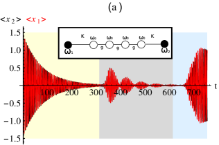
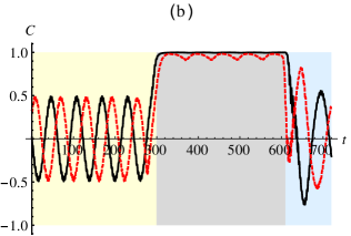
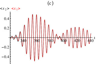
Figure 3: (a) Dynamics, (b) synchronization measure $C(t)$ and (c) zoomed view of the dynamics for two uncoupled oscillators ($\lambda=0$), with detuning $\delta\omega/\omega_{1}=0.1$ coupled to the extremities of the oscillator chain with coupling constant $K=0.2\,\omega_{1}^{2}$ and $M=300$, $\Omega_{0}=0.4\,\omega_{1}$ and $g=1.2\,\omega_{1}^{2}$. The inset in plot (a) shows a schematic representation of the configuration under analysis. Plot (b) shows the synchronization measure for two different initial conditions: symmetric $x_{1}(0)=x_{2}(0)=1.4\,\omega_{1}^{-1/2}$ and $p_{1}(0)=p_{2}(0)=0$ (solid black line) and asymmetric $x_{1}(0)=x_{2}(0)=2\,\omega_{1}^{-1/2}$ and $p_{1}(0)=0$, $=p_{2}(0)=10\,\sqrt{\omega_{1}}$ (dashed, red line). Plot (c) shows the dynamics of the two oscillators $\langle x_{1}(t)\rangle$ (solid black line) and $\langle x_{2}(t)\rangle$ (dashed red line), for a time window where synchronization appears. The background colors in plot (a) and (b) are inserted as a guide for the eye to mark the three region of independent dissipation (pink), cross-talk (blue) and revival (light blue). $\langle x_{1,2}\rangle$ are in units of $\omega_{1}^{-1/2}$ and time in units of $\omega_{1}^{-1}$.

During an initial transient, even if the probes are attached to the same environment (the chain), there are not decoherence free sub-spaces CBSB : the probes actually experience independent dissipation, the $\eta$ kernel vanishes, and $x_{+}$ and $x_{-}$ are coupled to orthogonal modes of the chain. During this transient the system oscillators lose energy and do not synchronize, as shown in Fig.3(a) and (b). This is consistent with previous studies with infinite and separate environments sync2012 .

In the weak coupling regime, the undamped oscillators start to feel the effect of each other after the time interval needed for signal propagation through the system, but their dynamics still remain incoherent. On the other hand, for stronger dissipation $K\lesssim\omega_{1,2}^{2}$ a sudden rise-up of the system oscillations appears at the cross-talk time $\tau_{CT}=\tau_{R}/2$ and perfect synchronization emerges. This behavior is illustrated in Fig. 3, in the central regions of panels (a) and (b). For $t>\tau_{R}$ each oscillator starts receive its own feedback and synchronization is lost again, since it is driven back to its natural frequency.

The mechanism of synchronization found in this regime consists of a reciprocal driving force of the two system HOs after their local damping: at $\tau_{CT}$ they have lost their initial energy due to their dissipation into the cold chain ($K=0.2\,\omega_{1}^{2}$ in Fig.3), and in the cross-talk time window $\tau_{CT}<t<\tau_{R}$ they receive a signal from the opposite (detuned) system oscillator. A driving at the frequency of the opposite oscillator, being detuned, would not cause any synchronization, but actually the exchanged signals are not at a single frequency, having a broad bandwidth due to the transmission through the chain. We find that, within the cross-talk time window, the oscillator $1$ is driven by a signal containing both the main frequency component $\omega_{2}^{\prime}$ primes and the resonant one $\omega_{1}^{\prime}$ (present in the broad signal transmitted through the chain), leading to the beating signal observed in Fig.3(c). A similar scenario occurs for the other oscillator $2$, now with the strongest and resonant frequency component exchanged. Therefore the oscillators placed at the edges, during cross-talk time, experience a driving force at a signal with the two detuned frequencies, leading to the characteristic beating signal of Fig.3 and to perfect synchronization.

This mechanism of synchronization for cross-talk is based on a reciprocal effect between the system components and is robust when breaking the symmetry in the initial conditions, even though in this case $delayed$ synchronization arises. Indeed for non-identical initial states $\{x_{1}(0),p_{1}(0)\}$ and $\{x_{2}(0),p_{2}(0)\}$, the respective signals experience a relative phase delay. Time delay can be taken into account considering the delayed signals $\langle x_{1}(t)\rangle$ and $\langle x_{2}(t+\Delta t)\rangle$ in $C$. Since this synchronization scenario is very sensitive to the initial conditions, both anti-synchronization and synchronization may arise.

V Synchronization and quantum correlations

An interesting question to answer is whether the emergence of synchronization is accompanied by an increase in the quantum or classical correlations in the system and if the mechanism of synchronization by dissipation (Sect. III.1) may be a witness for the appearance of robust quantum correlations and entanglement between the oscillators pair. As first reported in sync2012 starting from an entangled state weakly dissipating into the environment, decoherence and deterioration of quantum correlations will be reduced in presence of synchronization. This mechanism has been analysed also for 3 oscillators syncLalo and in networks syncSR .

Here we consider instead the possibility to create correlations and entanglement starting from product states of the system oscillators and in relation with quantum synchronization. To this purpose we consider uncoupled system oscillators starting from an uncorrelated (product) state with local squeezing. For identical oscillators $\omega_{1}=\omega_{2}$, entanglement mediated by the reservoir chain and its dynamical (sudden-death and revival) features have been predicted in Refs. morigiY ; morigiEPL in symmetric models. The possibility to entangle two oscillators due to strong dissipation in a common bath was addressed in correa while in syncSR the case of dissipative network was treated. The question we are interested here is the possibility to create entanglement due to the coherent energy transmission across the environment between detuned oscillators and in relation with spontaneous synchronization. The cases of interest are for system coupling mediated by the chain ($\lambda=0$)

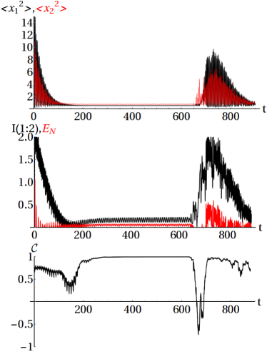
Figure 4: (From top to bottom) Quadratures, mutual information and entanglement, and synchronization factor, starting from a separable, squeezed state with squeezing parameters $r_{1}=r_{2}=2$, frequencies $\omega_{2}/\omega_{1}=1.2$ and coupling $\lambda=0$. The two oscillators are strongly coupled to the reservoir $K=0.8\,\omega_{1}^{2}$, and bath parameters are as in previous figures. $\langle x_{1,2}^{2}\rangle$ are in units of $\omega_{1}^{-1}$ and time in units of $\omega_{1}^{-1}$.

We monitor the system entanglement given by the logarithmic negativity $\mathcal{E}=\max(0,-\ln\nu)$, with $\nu$ the smallest symplectic eigenvalue of the partially transposed density matrix horodecki_review . Further we consider the mutual information $\mathcal{M}=S_{A}+S_{B}-S_{AB}$ with $S_{i}$ Von Neumann entropy of the reduced system $i=1,2$ and $S_{AB}$ the total entropy. Actually the latter has been also suggested to be an order parameter for quantum synchronization fazio2 .

V.1 Coupling to a common chain node

For a system plugged at the same point of a chain we have seen that two otherwise uncoupled oscillators ($\lambda=0$) can synchronize in the strong coupling regime due to the mediating effect of the environment (see Sect.IV.1). We find that this synchronization scenario is also present for system oscillators in vacuum squeezed states. In this case synchronization arises between the second order moments, as shown in Fig. 4. As for the case of average positions, fluctuations synchronization is allowed by the strong dissipation, Fig. 4a, and it later (at $\tau_{R}$) deteriorates due to feedback effects. Initially both MI and entanglement are established between the decoupled and initially uncorrelated system oscillators, as expected, due to their strong coupling mediated by the chain and the initial local squeezing, Fig. 4b. After a transient oscillatory decay $\mathcal{E}$ and $\mathcal{M}$ both reach a steady $non-vanishing$ value, consistently with predictions in Ref.correa . Here also synchronization appears, as shown in Fig. 4c, and actually witnesses entanglement.

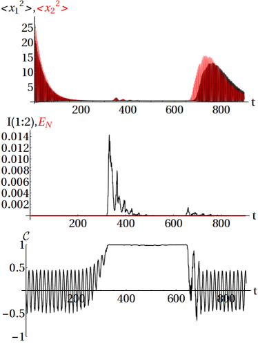
Figure 5: (From top to bottom) Position variances (top), mutual information and entanglement (middle), and synchronization factor (bottom), starting from a separable, squeezed state with squeezing parameters $r_{1}=r_{2}=2$, frequencies $\omega_{2}/\omega_{1}=1.2$ and coupling $\lambda=0$. The coupling to the reservoir is $K=0.2\,\omega_{1}^{2}$, and bath parameters are as in previous figures. $\langle x_{1,2}^{2}\rangle$ are in units of $\omega_{1}^{-1}$ and time in units of $\omega_{1}^{-1}$.

This microscopic model shows that strong coupling to a common environment allows to synchronize and entangle uncoupled detuned oscillators whose interaction is mediated by the environment. This would persists for an infinite bath while feed-back effects in a finite model case hinder synchronization, Fig. 4c for $t>\tau_{R}$. Further we notice that the increase of mutual information at $\tau_{R}$ does not always reflect dynamical synchronization that at the contrary can decay ($\mathcal{C}\simeq 0$ for $650<\omega_{1}t<700$).

The fact that two uncoupled oscillators, interacting with a chain, evolve into a synchronized and entangled state is a distinctive effect of strong coupling, which is not present for weak coupling.

V.2 Coupling to the chain edges

We now consider the case in which the oscillators are far-apart, at the opposite edges of the chain as in Sect. IV.2. Is it possible to synchronize their quantum fluctuations and entangle them due to the cross-talk? We consider again squeezed vacuum states, observing that the system probes at the opposite edges of the chain evolve toward a quantum synchronized state in its fluctuations, with a build-up of correlations during the cross-talk time, as shown by their mutual information rising from vanishing to finite values (Fig. 5). Nevertheless, for reasonable values of the initial squeezing, entanglement is never created, independently on the initial squeezing strength. For distant probes therefore synchronization may emerge when in a cross-talk regime where they exchange energy but this does not lead to entanglement.

VI Conclusions

In conclusion, we have addressed synchronization of two quantum oscillators within a finite linear system, and analyzed in details the possible mechanisms leading to a coherent dynamics of the (detuned) system components. Besides, we have analyzed in some details the connections of synchronization with the build up of entanglement starting from uncorrelated states and without any direct coupling between the two oscillators.

Our microscopic description has allowed us to go beyond the weak dissipation limit, showing that in the strong coupling regime new synchronization mechanisms appears among uncoupled oscillators, leading to coherent dynamics enabled by the environment. Furthermore, cross-talk effects may have a constructive role, inducing synchronization mediated by signal transmission. More in general, a condition for spontaneous synchronization of linear oscillators has been discussed in the context of the Rayleigh model for vibrations physics.

As a matter of fact, synchronization is important in different contexts but not always desirable. For quantum networks syncSR , quantum synchronization witnesses the presence of quantum correlations which are more robust against dissipation, and even the appearance of noiseless sub-systems. On the other hand, in the context of physics of vibrations, the fact that some vibration modes are damped out very slowly may compromise the stability of complex structures vibrations .

Our results pave the way to the analysis of local synchronization mechanisms for small clusters within a larger network, and to applications of interest for quantum technology and metrology, e.g. the use of spontaneous synchronization to witness quantum correlations or the synchronization of clocks by coherent coupling.

Appendix A Hamiltonian normal modes and Langevin equation

Let’s consider a system of two quantum harmonic oscillators, characterized by frequencies $\omega_{1}$ and $\omega_{2}$ and coupling strength $\lambda$ between them. The oscillators are plugged with strength $K$ into an homogeneous chain of quantum HOs at frequency $\Omega_{0}$ and chain stiffness $g$. We now introduce the notation used to describe the system and environment normal modes (NM):

$$H_{S} =\frac{\tilde{p_{1}}^{2}}{2}+\frac{\tilde{p_{2}}^{2}}{2}+\frac{1}{2}\Lambda^{2}_{-}q_{1}^{2}+\frac{1}{2}\Lambda^{2}_{+}q_{2}^{2}$$ (11)

$$H_{E} =\sum_{j=1}^{M}\left[\frac{\tilde{P}_{j}^{2}}{2}+\frac{1}{2}\Omega^{2}_{j}Q_{j}^{2}\right]$$ (12)

$$H_{I} =q_{1}\sum_{j=1}^{M}c_{1}(j)Q_{j}+q_{2}\sum_{j=1}^{M}c_{2}(j)Q_{j}.$$ (13)

where the positions normal modes operators are denoted by $q_{1,2}$ for the system and $Q_{j}$ for the environment and are computed as:

$$q_{1} =\cos\theta\;x_{1}+\sin\theta\;x_{2}$$ (14)

$$q_{2} =-\sin\theta\;x_{1}+\cos\theta\;x_{2}$$ (15)

$$X_{j} =\sqrt{\frac{2}{M+1}}\sum_{k=0}^{M}\sin\left(\frac{\pi kj}{M+1}\right)Q_{k}$$ (16)

where the quantity $\theta$ is defined by the relation

$$\tan(2\theta)=\frac{2\lambda}{\omega_{2}^{2}-\omega_{1}^{2}}.$$

The eigenfrequencies and the coupling coefficients are given by:

$$\Lambda^{2}_{s}=\lambda+\frac{\omega_{1}^{2}+\omega_{2}^{2}}{2}\,+\frac{(-1)^{s}}{2}\sqrt{4\lambda^{2}+\left(\omega_{1}^{2}-\omega_{2}^{2}\right)^{2}}$$ (17)

$$\Omega^{2}_{j}=\Omega_{0}^{2}+4g\sin^{2}\left(\frac{\pi j}{2(M+1)}\right)$$ (18)

$$c_{1}(j)=\sqrt{\frac{2K^{2}}{M+1}}\;\;\times$$

$$\hskip 19.91684pt\left[\cos\theta\sin\left(\frac{\pi jm}{M+1}\right)+\sin\theta\sin\left(\frac{\pi jn}{M+1}\right)\right]$$ (19)

$$c_{2}(j)=\sqrt{\frac{2K^{2}}{M+1}}\;\;\times$$

$$\hskip 19.91684pt\left[\cos\theta\sin\left(\frac{\pi jn}{M+1}\right)-\sin\theta\sin\left(\frac{\pi jm}{M+1}\right)\right].$$ (20)

The dynamics of the system is described by a generalized quantum Langevin equations (GQLE) for operators $q_{1}(t)$ and $q_{2}(t)$, obtained starting from the set of Heisenberg equations for system and environment operators $\{q_{1(2)},\tilde{p}_{1(2)},Q_{j},\tilde{P}_{j}\}$. The GQLE are integro-differential equations that describe the dynamics of the NM operators as a function of the environment parameters and coupling constants:

$$\ddot{q}_{1}(t)+[\Lambda^{2}_{1}-\gamma_{1}(0)]q_{1}(t)$$

$$+\int_{0}^{t}dt^{\prime}[\gamma_{1}(t-t^{\prime})\dot{q}_{1}(t^{\prime})+\eta(t-t^{\prime})\dot{q}_{2}(t^{\prime})]$$

$$=-\xi_{1}(t)-\gamma_{1}(t)q_{1}(0)-\eta(t)q_{2}(0)+\eta(0)q_{2}(t)$$ (21)

and an equivalent expression is found for operator $q_{2}$ by replacing $1\longleftrightarrow 2$. The kernels $\gamma$ and $\eta$ take the expressions:

$$\gamma_{s} (t-t^{\prime})=\sum_{j=1}^{M}\frac{c_{s}^{2}(j)}{\Omega_{j}^{2}}\cos[\Omega_{j}(t-t^{\prime})]\Theta(t-t^{\prime})$$ (22)

$$\eta (t-t^{\prime})=$$

$$=\sum_{j=1}^{M}\frac{c_{1}(j)c_{2}(j)}{\Omega_{j}^{2}}\cos[\Omega_{j}(t-t^{\prime})]\Theta(t-t^{\prime})$$ (23)

where $s=1,2$ and the external force operator $\xi_{1(2)}(t)$ depends upon the environment initial conditions

$$\xi_{s}(t)=$$

$$=\sum_{j}c_{s}(j)\left(Q_{j}(0)\cos(\Omega_{j}t)+\frac{P_{j}(0)}{\Omega_{j}}\sin(\Omega_{j}t)\right)$$ (24)

and gives a zero contribution when averaged over the vacuum state of the environment.

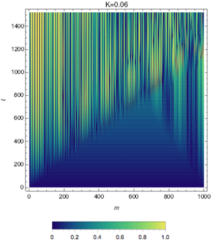
Figure 6: Density plot of the synchronization measure $C(t)$ for a 300-site chain as a function of the plugging site $m$ and the time $t$. The parameters are set as: $\omega_{2}/\omega_{1}=1.1$, $\lambda=0.5\,\omega_{1}^{2}$, $K=0.06\,\omega_{1}^{2}$, $\Omega_{0}=0.4\,\omega_{1}$ and $g=1.2\,\omega_{1}^{2}$.

Appendix B Synchronization across the chain: case $0\ll m\ll N$

When moving the second oscillator through the chain but far from the edges, i.e. $0\ll m\ll N$, there is an initial time transient in which the oscillators do not synchronize and this behavior is independent on the position $m$, as shown in Fig.6. This occurs only before cross-talk and feedback from the boundaries take place and actually corresponds to a good approximation of independent dissipation of the two detuned systems. In particular, if the coupling is weak and time is long enough to have only the resonant system-bath interaction surviving, then one expects that the chain normal modes $Q_{k}\pm$ that are resonant with the system eigenfrequencies dominate the dynamics ($k_{-}$ resonates with the system normal mode $q_{1}$ and $k_{+}$ with $q_{2}$) leading to an effective interaction

$$H_{I}=K\sqrt{\frac{2}{M+1}}\left[c_{1}q_{1}Q_{k_{-}}+c_{2}q_{2}Q_{k_{+}}\right].$$ (25)

with

$$c_{1}=\left[\cos\theta\;\sin\left(\frac{\pi k_{-}}{M+1}\right)+\sin\theta\;\sin\left(\frac{\pi k_{-}m}{M+1}\right)\right]$$ (26)

$$c_{2}=\left[\cos\theta\;\sin\left(\frac{\pi k_{+}m}{M+1}\right)-\sin\theta\;\sin\left(\frac{\pi k_{+}}{M+1}\right)\right]$$ (27)

Nevertheless, such effective resonant interaction is established after long times, while during the transient analyzed here there are bands of normal modes that are exchanging energy with the system. The average effect of several of such modes of the chain leads to $c_{1}\sim\cos\theta\;\sin\left(\frac{\pi k_{-}}{M+1}\right)$ and $c_{2}\sim\sin\theta\;\sin\left(\frac{\pi k_{+}}{M+1}\right)$, so that the system normal modes decay at some rate independently on their distance $m$, as shown in the triangular region in Fig. 6. The spatio-temporal synchronization diagram shown in Fig. 6 clearly displays the effects of cross-talk and reflections from the boundaries, leading to a strong and non-monotonic dependence on $m$ and, often, to synchronization for larger times.

References

- (1) G. Heinrich, M. Ludwig, J. Qian, B. Kubala, and F. Marquardt, Phys. Rev. Lett. 107, 043603 (2011); M. Ludwig and F. Marquardt, Phys. Rev. Lett. 111, 073603 (2013).
- (2) G. L. Giorgi, F. Galve, G. Manzano, P. Colet, and R. Zambrini, Phys. Rev. A 85, 052101 (2012).
- (3) G.Manzano, F. Galve, G. L. Giorgi, E. Hernandez-Garcia, and R. Zambrini, Sci. Rep. 3, 1439 (2013).
- (4) A. Mari, A. Farace, N. Didier, V. Giovannetti, and R. Fazio, Phys. Rev. Lett. 111, 103605 (2013).
- (5) S. H. Strogatz and I. Stewart, Sci. Am. 267, No. 6, 102. (1993)
- (6) G. V. Osipov, J. Kurths, and C. Zhou, Synchronization in oscillatory networks (Springer, Berlin, 2007).
- (7) A. Pikovsky, M. Rosenblum, and J. Kurths, Synchronization: A Universal Concept in Nonlinear Sciences (Cambridge Univ. Press, Cambridge, 2001).
- (8) S. H. Strogatz, Nonlinear Dynamics And Chaos: With Applications To Physics, Biology, Chemistry, And Engineering (Westview Press, Boulder, 2001)
- (9) S.C. Manrubia, A.S. Mikhailov, and D.H. Zanette, Emergence of Dynamical Order. Synchronization Phenomena in Complex Systems, Lect. Not. Compl. Syst. 2 (World Scientic, Singapore, 2004).
- (10) F. Galve, G.L. Giorgi and R. Zambrini, chapter Quantum correlations and synchronization measures, to appear in ”Lectures on general quantum correlations and their applications”, Springer (2016)
- (11) G. Manzano, F. Galve, and R. Zambrini, Phys. Rev. A 87, 032114 (2013).
- (12) U. Weiss, Quantum Dissipative Systems (World Scientific Publishing, Singapore, 2008); H.-P. Breuer and F. Petruccione, The Theory of Open Quantum Systems (Oxford Univ. Press, 2007); C.W. Gardiner and P. Zoller, Quantum Noise, (Springer, Berlin 2004).
- (13) A. Arenas, A. Diaz-Guilera, J. Kurths, Y. Moreno, and C. Zhou, Phys. Rep. 469, 93 (2008).
- (14) K. R. Brown, C. Ospelkaus, Y. Colombe, A. C. Wilson, D. Leibfried, and D. J. Wineland, Nature 471, 196 (2011); M. Harlander, R. Lechner, M. Brownnutt, R. Blatt, and W. Hansel, Nature 471, 200 (2011); M. R. Hush, W. Li, S. Genway, I. Lesanovsky, and A. D. Armour, Phys. Rev. A 91, 061401(R) (2015).
- (15) R. Vasile, F. Galve, and R. Zambrini, Phys. Rev. A 89, 022109 (2014).
- (16) A. W. Chin, A. Rivas, S. F. Huelga, and M. B. Plenio, J. Math. Phys. 51, 092109 (2010); R. Martinazzo, B. Vacchini, K. H. Hughes, and I. Burghardt, J. Chem. Phys. 134, 011101 (2011).
- (17) J. Nokkala, F. Galve, R. Zambrini, S. Maniscalco, and J. Piilo, Sci. Rep. 6, 26861 (2016).
- (18) Á. Rivas, S. F. Huelga, and M. B. Plenio, Rep. Prog. Phys. 77 094001 (2014); I. de Vega, D. Alonso, arXiv:1511.06994.
- (19) I. de Vega, Phys. Rev. A 90, 043806 (2014).
- (20) F. Galve, A. Mandarino, M. G. A. Paris, C. Benedetti, and R. Zambrini, ArXiv:1606.03390 and references therein.
- (21) E. Kajari, A. Wolf, E. Lutz, and G. Morigi, Phys. Rev. A 85, 042318 (2012).
- (22) A. Wolf, G. De Chiara, E. Kajari, E. Lutz, and G. Morigi, Europhys. Lett. 95, 60008 (2011); T. Fogarty, E. Kajari, B. G. Taketani, A. Wolf, Th. Busch, and G. Morigi, Phys. Rev. A 87, 050304 (2013).
- (23) T. Zell, F. Queisser, and R. Klesse, Phys. Rev. Lett. 102, 160501 (2009).
- (24) L. A. Correa, A. A. Valido, and D. Alonso, Phys. Rev. A 86, 012110 (2012).
- (25) V. Ameri, M. Eghbali-Arani, A. Mari, A. Farace, F. Kheirandish, V. Giovannetti, and R. Fazio, Phys. Rev. A 91, 012301 (2015).
- (26) P. Hanggi and G.-L. Ingold, Chaos 15, 026105 (2005).
- (27) J.F. Kimble in Fundamental Systems in Quantum Optics (Les Houches, Session LIII, 1990. Elsevier, 1992), pg.545-674.
- (28) R. J. Rubin, Phys. Rev. 131, 964 (1963).
- (29) H.-P. Breuer, E.-M. Laine, J. Piilo, B. Vacchini, Rev. Mod. Phys. 88, 021002 (2016).
- (30) J. K. Knowles, Struct. Control Health Monit. 13, 324 (2006); T. Balendra, C. W. Tat, and S. L. Lee, Earthquake Engng. Struct. Dyn., 10, 735 (1982).
- (31) J. W. Strutt (Lord Rayleigh) The Theory of Sound,Vol.1, second ed., (Dover, New York, 1945).
- (32) T. K. Caughey, J. Appl. Mech. 27, 269 (1960); T. K. Caughey , M. E. J. O’Kelly, J. Appl. Mech. 32, 583 (1965).
- (33) Here ‘classical’ is the adopted terminology used in vibration physics, not to be confused with the absence of quantumness.
- (34) G. L. Giorgi, F. Plastina, G. Francica, and R. Zambrini, Physical Review A 88, 042115 (2013).
- (35) R. Horodecki, P. Horodecki, M. Horodecki, and K. Horodecki, Rev. Mod. Phys. 81, 865 (2009).
- (36) F. Galve and R. Zambrini, Int. J. Quantum Inf. 12, 1560022 (2014).
- (37) B. G. Taketani, T. Fogarty, E. Kajari, T. Busch, and G. Morigi, Phys. Rev. A 90, 012312 (2014).
- (38) Primed frequencies include the Lamb shifted due to coupling with the chain.
- (39) F. Galve, G. L. Giorgi, and R. Zambrini, Phys. Rev. A 81, 062117 (2010).